Quantum correlations dynamics under different non-markovian environmental models

Abstract

We investigate the roles of different environmental models on quantum correlation dynamics of two-qubit composite system interacting with two independent environments. The most common environmental models (the single-Lorentzian model, the squared-Lorentzian model, the two-Lorentzian model and band-gap model) are analyzed. First, we note that for the weak coupling regime, the monotonous decay speed of the quantum correlation is mainly determined by the spectral density functions of these different environments. Then, by considering the strong coupling regime we find that, contrary to what is stated in the weak coupling regime, the dynamics of quantum correlation depends on the non-Markovianity of the environmental models, and is independent of the environmental spectrum density functions.

I INTRODUCTION

Until recently a lot of interest has been devoted to the definition and understanding the quantum aspects of correlation in a composite system. The discovery that mixed separable (unentangled) states can have nonclassical correlation [1-4] and such states provide computational speedup compared to classical states in some quantum computation models [4,5]. In order to quantify the quantumness of the correlation contained in a bipartite quantum state Olliver and Zurek [3] proposed a measure for quantum correlation known as quantum discord (QD) and based on a distinction between quantum information theory and classical information theory. A recent result that almost all quantum states have a nonvanishing QD [6] shows up the relavance of studying such correlation.
Besides the quantification of quantum correlations, another important problem is the behavior of these correlations under the action of decoherence. The phenomenon, caused by the injection of noise into the system and arising from its inevitable interaction with the surrounding environment, is responsible for the loss of quantum coherence initially present in the system. Recently it was noted that the dynamical behaviors of QD in the presence of the Markovian [7,8] decoherence decay exponentially in time and vanish only asymptotically [9,10], contrary to the entanglement dynamics where sudden death may occur [11-18]. In these above studies, the quantumness of correlation is more robust to the action of the environment than the entanglement itself. In particular, Refs. [19,20] have discovered that the QD can be completely unaffected by Markovian depolarizing channels or non-Markovian depolarizing channels for long intervals of time, and this phenomenon has been observed experimentally [21]. As Refs. [19-21], it is of interest to find a certain environmental model that the quantum correlation can be unaffected by decoherence as much as possible.
In this article, we will concentrate on the question: what kind of local environmental model can make the initial quantum correlation more robust in the dynamics process? We consider a noninteracting two-qubit system under the influence of two independent environments. The most common environmental models (the single-Lorentzian model, the squared-Lorentzian model, the two-Lorentzian model and band-gap model) are studied. By analytical and numerical analysis we find that, for the weak coupling regime, the monotonous decay speed of the two-qubit QD is mainly determined by the spectral density functions of these different environments. The two-qubit QD in the single-Lorentzian (band-gap) environment is more robust than in the squared-Lorentzian (two-Lorentzian) environment under the resonant and near resonant conditions. While for the far off-resonant condition the two-qubit QD in the single-Lorentzian (band-gap) environment decreases much more faster than in the squared-Lorentzian (two-Lorentzian) environment. However, by considering the strong coupling regime we find that, the two-qubit QD is more robust in the squared-Lorentzian (two-Lorentzian) environment than in the single-Lorentzian (band-gap) environment, either under the near resonant or far off-resonant condition. In this case, the dynamics of QD mainly depends on the non-Markovianity of the environmental models, and is independent of the environmental spectrum density functions.

II Theoretical model and dynamics of two-qubit system

Considering a model consisting of two qubits $A$ and $B$, each interacting with a zero-temperature bosonic environment, denoted $a$ and $b$, respectively, we assume that each qubit-environment system is isolated and the environments are initially in the vacuum state while two qubits are initially in an quantum correlated state. A specific system which consists of two independent two-level atoms interacting with an multi-mode environment respectively has been chosen in this paper. Since each atom evolves independently, we can learn how to characterize the evolution of the overall system from the atom-environment dynamics. The interaction between an atom and an N-mode environment in the rotating-wave approximation is given by $H^{j}_{0}+H^{j}_{int}$, which, in the basis $\{|gg\rangle,|ge\rangle,|eg\rangle,|ee\rangle\}$, reads

$$\hat{H}^{j}_{0} = \omega_{0}\hat{\sigma}^{j}_{+}\hat{\sigma}^{j}_{-}+\sum_{k=1}^{N}\omega_{k}a^{{\dagger}}_{k}a_{k},$$ (1)

$$\hat{H}^{j}_{int} = \sum_{k=1}^{N}g_{k}(\hat{\sigma}^{j}_{+}a_{k}+\hat{\sigma}^{j}_{-}a^{{\dagger}}_{k}),$$ (2)

here $a^{{\dagger}}_{k}$, $a_{k}$ are the creation and annihilation operators of quanta of the environment ($a$ or $b$), $\hat{\sigma}^{j}_{+}=|e_{j}{\rangle}{\langle}g_{j}|$, $\hat{\sigma}^{j}_{-}=|g_{j}{\rangle}{\langle}e_{j}|$ and $\omega_{j}$ are the inversion operators and transition frequency of the $j$-th atom (j=$A$, $B$ and here $\omega_{A}=\omega_{B}=\omega_{0}$ ); $\omega_{k}$ and $g_{k}$ are the frequency of the mode $k$ of the environment and its coupling strength with the atom. To illustrate the roles of the different environmental models on quantum correlation dynamics of two atoms, we assume that two atoms interact off-resonantly with their structured environment, whose spectral density function $D(\omega)$ provides a complete characterization of the evolution for single-Lorentzian, two-Lorentzian, band-gap and squared-Lorentzian environments.
In order to find the atom-environment dynamics, we solve the master equation by using the pseudomode approach [22,23]. This exact master equation describes the coherent interaction between the atom and the pseudomodes in the presence of the decay of the pseudomodes due to the interaction with a Markovian reservoir [24]. The number of the pseudomodes relies on the shape of the environmemt spectral density function. $(a)$ For the single-Lorentzian environmental model $D(\omega)=\frac{\Gamma}{(\omega-\omega_{c})^{2}+(\Gamma/2)^{2}}$, there has only one pole in the lower half complex plane, the atom interacts with one pseudomode which leaks into a Markovian environment. So the exact dynamics of the atom interacting with a single-Lorentzian structured environment is contained in the following pseudomode master equation

$$\frac{d\rho}{dt}=-i[H^{j},\rho]-\frac{\Gamma}{2}[a^{{\dagger}}a\rho-2a{\rho}a^{{\dagger}}+{\rho}a^{{\dagger}}a],$$ (3)

where

$$H^{j}=\omega_{0}\sigma^{j}_{+}\sigma^{j}_{-}+\omega_{c}a^{{\dagger}}a+\Omega(\sigma^{j}_{+}a+\sigma^{j}_{-}a^{{\dagger}}),$$ (4)

with $\rho$ is the density operator for the $j$-th atom and the pseudomode of the structured reservoir, $a$ and $a^{{\dagger}}$ are the annihilation and creation operators of the pseudomode. The constants $\omega_{c}$ and $\Gamma$ are, respectively, the oscillation frequency and the decay rate of the pseudomode and they depend on the position of the pole $z\equiv\omega_{c}-i\Gamma/2$. The $j$-th atom interacts coherently with the pseudomode (the strength of the coupling $\Omega$).
$(b)$ According to the two-Lorentzian environmental model, the environment spectral density function is simply a sum of two Lorentzian functions $D(\omega)=W_{1}\frac{\Gamma_{1}}{(\omega-\omega_{c})^{2}+(\Gamma_{1}/2)^{2}}+W_{2}\frac{\Gamma_{2}}{(\omega-\omega_{c})^{2}+(\Gamma_{2}/2)^{2}}$, where the weights of the two Lorentzians are such that $W_{1}+W_{2}=1$. There are two poles in the lower half complex plane, the atom interacts with two pseudomodes ($a_{1}$ and $a_{2}$) which leak into a Markovian environment ($\Gamma_{1}$ and $\Gamma_{2}$ are the decay rates), respectively. This time the poles are located at $z_{1}=\omega_{c}-i\Gamma_{1}/2$ and $z_{2}=\omega_{c}-i\Gamma_{2}/2$, so the exact master equation for the atom-environment dynamics in the two-Lorentzian environmental model can be written

$$\frac{d\rho}{dt}= - i[H^{j},\rho]-\frac{\Gamma_{1}}{2}(a^{{\dagger}}_{1}a_{1}\rho-2a_{1}{\rho}a^{{\dagger}}_{1}+{\rho}a^{{\dagger}}_{1}a_{1})$$ (5)

$$- \frac{\Gamma_{2}}{2}(a^{{\dagger}}_{2}a_{2}\rho-2a_{2}{\rho}a^{{\dagger}}_{2}+{\rho}a^{{\dagger}}_{2}a_{2}),$$

and here

$$H^{j}= \omega_{0} \sigma^{j}_{+}\sigma^{j}_{-}+\omega_{c}a^{{\dagger}}_{1}a_{1}+\omega_{c}a^{{\dagger}}_{2}a_{2}+\Omega\sqrt{W_{1}}(\sigma^{j}_{+}a_{1}$$ (6)

$$+ \sigma^{j}_{-}a^{{\dagger}}_{1})+\Omega\sqrt{W_{2}}(\sigma^{j}_{+}a_{2}+\sigma^{j}_{-}a^{{\dagger}}_{2}).$$

$(c)$ Next we give an idealized model of a band gap (or photon density of states gap) $D(\omega)=\frac{W_{1}\Gamma_{1}}{(\omega-\omega_{c})^{2}+(\frac{\Gamma_{1}}{2})^{2}}-\frac{W_{2}\Gamma_{2}}{(\omega-\omega_{c})^{2}+(\frac{\Gamma_{2}}{2})^{2}}$ in which both Lorentzians are centered at the same frequency, the second is given a negative weight, and the weights of the two Lorentzians are such that $W_{1}-W_{2}=1$ and $\Gamma_{2}<\Gamma_{1}$ ensure positivity of $D(\omega)$. There also have two poles in the lower half complex plane as the two-Lorentzian model, the two poles are located at $\omega_{c}-i\Gamma_{1}/2$ and $\omega_{c}-i\Gamma_{2}/2$, so there are also two pseudomodes $a_{1}$ and $a_{2}$ with deacy rates $\Gamma^{\prime}_{1}=W_{1}\Gamma_{2}-W_{2}\Gamma_{1}$ and $\Gamma^{\prime}_{2}=W_{1}\Gamma_{1}-W_{2}\Gamma_{2}$ respectively. The $j$-th atom does not couple to the first pseudomode $a_{1}$ at all, it only interacts coherently with the second pseudomode $a_{2}$ (the strength of the coupling $\Omega$) which is in turn coupled to the first one (the strength of the coupling $V=\sqrt{W_{1}W_{2}}(\Gamma_{1}-\Gamma_{2})/2$), and both pseudomodes are leaking into independent Markovian environments. The exact pseudomode master equation associated with the band-gap model is given by

$$\frac{d\rho}{dt}= - i[H^{j},\rho]-\frac{\Gamma^{\prime}_{1}}{2}[a^{{\dagger}}_{1}a_{1}\rho-2a_{1}{\rho}a^{{\dagger}}_{1}+{\rho}a^{{\dagger}}_{1}a_{1}]$$ (7)

$$- \frac{\Gamma^{\prime}_{2}}{2}[a^{{\dagger}}_{2}a_{2}\rho-2a_{2}{\rho}a^{{\dagger}}_{2}+{\rho}a^{{\dagger}}_{2}a_{2}],$$

where

$$H^{j} = \omega_{0}\sigma^{j}_{+}\sigma^{j}_{-}+\omega_{c}a^{{\dagger}}_{1}a_{1}+\omega_{c}a^{{\dagger}}_{2}a_{2}+\Omega(a^{{\dagger}}_{2}\sigma^{j}_{-}$$ (8)

$$+ a_{2}\sigma^{j}_{+})+V(a^{{\dagger}}_{1}a_{2}+a_{1}a^{{\dagger}}_{2}).$$

$(d)$ The environment spectral density function of the squared-Lorentzian model is $D(\omega)=\frac{\Gamma^{3}/2}{[(\omega-\omega_{c})^{2}+(\Gamma/2)^{2}]^{2}}$, for which we will find that there exist two pseudomodes $a_{1}$ and $a_{2}$, and the $j$-th atom only couples to the second pseudomode $a_{2}$ (the coupling constant $\Omega$) which interacts with the first pseudomode $a_{1}$ (the strength of the coupling $V=\Gamma/2$). Different from the band-gap model, only the first pseudomode will show any decay to the Markovian environment with decay rate $\Gamma$, the second pseudomode which is directly coupled to the $j$-th atom does not decay in this model. So the dynamics of the $j$-th atom and two pseudomodes obey the following master equation

$$\frac{d\rho}{dt}=-i[H^{j},\rho]-\Gamma[a^{{\dagger}}_{1}a_{1}\rho-2a_{1}{\rho}a^{{\dagger}}_{1}+{\rho}a^{{\dagger}}_{1}a_{1}],$$ (9)

with the Hamiltonian

$$H^{j} = \omega_{0}\sigma^{j}_{+}\sigma^{j}_{-}+\omega_{c}a^{{\dagger}}_{1}a_{1}+\omega_{c}a^{{\dagger}}_{2}a_{2}+\Omega(a^{{\dagger}}_{2}\sigma^{j}_{-}$$ (10)

$$+ a_{2}\sigma^{j}_{+})+V(a^{{\dagger}}_{1}a_{2}+a_{1}a^{{\dagger}}_{2}).$$

In order to analyze the roles of the different environmental models on quantum correlation dynamics of two atoms, we consider the above four environmental models, respectively, $i.e.,$ the single-Lorentzian model, two-Lorentzian model, band-gap model and squared-Lorentzian model. According to the above analysis, the spectral density functions of single-Lorentzian model and squared-Lorentzian model have a same parameter $\Gamma$, and the two-Lorentzian model and band-gap model both contain two Lorentzians, the same parameters ($W_{1}$, $W_{2}$, $\Gamma_{1}$ and $\Gamma_{2}$) appear in the spectral density functions of them. So in this paper we will mainly compare the difference in quantum correlation dynamics of two atoms between the single-Lorentzian model and squared-Lorentzian model, as well as bewteen the two-Lorentzian model and band-gap model. For an initial state of the total system $\rho(0)_{ABab}=|\Psi\rangle\langle\Psi|$, with $|\Psi\rangle=(\cos\theta|gg\rangle_{AB}+\sin\theta|ee\rangle_{AB})\otimes|\bar{0}\rangle_{a}|\bar{0}\rangle_{b}$, and here $\theta\in[0,\pi]$, $|e\rangle$ and $|g\rangle$ are the excited state and ground state of atoms, $|\bar{0}\rangle_{a,b}=\prod_{k=1}^{N}|0_{k}\rangle_{a,b}$ is the vacuum state of the environment $a,b$. Then the evolutional density matrix $\rho(t)$ of the total system in different environmental models can be acquired respectively by solving the above master equations (from Eqs. (3) to (10)). Tracing out the pseudomode degree of freedom, we obtain the reduced density matrix $\rho_{AB}(t)$ of the atomic system in these four different environmental models.
The measure of total quantum correlations used here is the quantum discord (QD) [3]. In all cases investigated in this paper the reduced density matrix for the atomic system $\rho_{AB}(t)$ in the basis $\{|gg\rangle,|ge\rangle,|eg\rangle,|ee\rangle\}$ has an $X$ structure defined by its elements $\rho_{12}=\rho_{13}=\rho_{24}=\rho_{34}=0$, $\rho_{22}=\rho_{33}$ and $\rho_{14}=\rho^{*}_{41}$. For this $X$ class of density matrix, QD can be calculated analytically [25]: $QD(\rho_{AB})=S(\rho_{B})+\sum^{3}_{j=0}\lambda_{j}\log_{2}\lambda_{j}+\min_{\{B_{i}\}}[S(\rho|\{B_{i}\})]$, where $\lambda_{j}$ is the $j$-th eigenvalue of the density matrix $\rho_{AB}(t)$. Here $S(\rho_{B})$ denotes the von Neumann entropy of $\rho_{B}=Tr_{A}\rho_{AB}$ and $S(\rho|\{B_{i}\})$ is the quantum conditional entropy with respect to a von Neumann measurement $\{B_{i}\}$ for subsystem $B$.

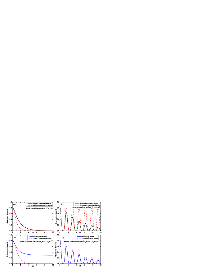
Figure 1: (Color online) Time evolution of the atomic QD as a function of the dimensionless quantity ${\Omega}t$ under the atom-pseudomode resonant condition ($\Delta=\omega_{c}-\omega_{0}=0$), with $\theta=\pi/3$. (a) and (b) the single-Lorentzian and squared-Lorentzian as the environmental models; (c) and (d) the two-Lorentzian and band-gap as the environmental models.

III Numerical results and discussions

In Figs. $1(a)$ and $1(b)$, by considering the atom-pseudomode resonant condition ($\Delta=\omega_{c}-\omega_{0}=0$) and choosing the single-Lorentzian model and squared-Lorentzian model as the environmental spectral density functions, we plot the time evolution of QD for two qubits as function of the dimensionless quantity ${\Omega}t$ in the weak coupling regime and the strong coupling regime, with $\theta=\pi/3$. In the weak coupling regime QD decays only asymptotically to zero while in the strong coupling regime the atomic QD presents damped oscillations. A comparison between the dark solid curve and the red dashed curve in Figs. $1(a)$ and $1(b)$ reveals that for the weak coupling regime, the atomic QD due to the single-Lorentzian environmental model is more robust than the case of the squared-Lorentzian model, but in the strong coupling regime, the atomic QD attenuates more slowly in the case of the squared-Lorentzian model than the single-Lorentzian model. Through comparing the atomic QD dynamics in the two-Lorentzian environmental model and band-gap environmental model (as shown in Figs. $1(c)$ and $1(d)$), we acquire that in the weak coupling regime, the QD can decrease to a long-time asymptotic value in the band-gap model while for the case of the two-Lorentzian model the QD can reduce eventually to zero. However, according to the strong coupling regime, the atomic QD is more robust in the case of the two-Lorentzian model than the band-gap model.
Then, in order to investigating the effects of different environmental models on the atomic QD under the atom-pseudomode near resonant and far off-resonant conditions, we analyze the evolution behavior of the QD in the weak coupling regime, by the comparison of two cases: near resonance condition ($\Delta=0.2\Omega$) and far off-resonance condition ($\Delta=8\Omega$), with $\theta=\pi/3$. For the case of near resonance, as shown in Figs. $2(a)$ and $2(c)$, one could find that the atomic QD in the single-Lorentzian (band-gap) environment is more robust than in the squared-Lorentzian (two-Lorentzian) environment. However, an opposite result that the atomic QD in the single-Lorentzian (band-gap) environment decreases much more faster than in the squared-Lorentzian (two-Lorentzian) environment are obtained for the far off-resonant condition, clearly seen in Figs. $2(b)$ and $2(d)$. What is the physics behind the phenomena? In this part we try to give an enlightening discussion for this problem based on these environmental models. Let us review the spectrum density functions of these models, as shown in Fig. $3$. The center part of the spectrum density function of the single-Lorentzian (band-gap) environment is much smaller than of the squared-Lorentzian (two-Lorentzian) environment. In contrast, the parts which are far from the center are larger in the single-Lorentzian (band-gap) environment than in the squared-Lorentzian (two-Lorentzian) environment. Thus, to determine in which environmental model the atomic QD is more robust in the weak coupling regime, we can compare the spectral density functions of these different environments: the decay behavior of the atomic QD is determined by the modes of the spectrum which are resonant with the atoms: the monotonous decay speed of the QD decreases as the density of these modes decreases.

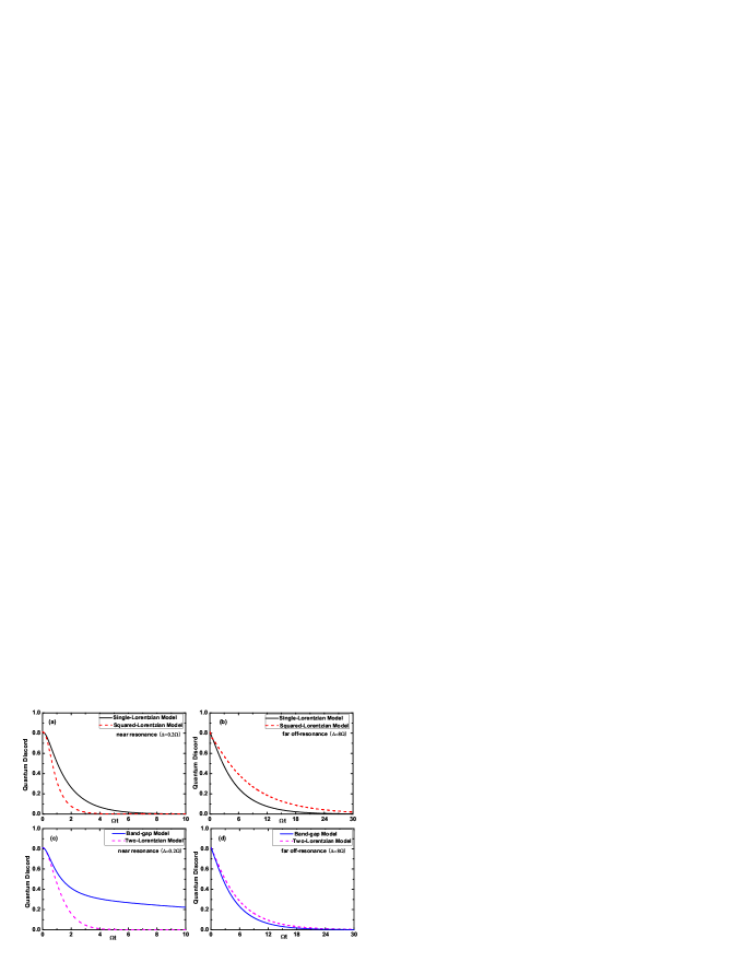
Figure 2: (Color online) Time evolution of the atomic QD as a function of the dimensionless quantity ${\Omega}t$ under the atom-pseudomode near resonance regime and far off-resonance regime, with $\theta=\pi/3$. (a) and (b) the single-Lorentzian and squared-Lorentzian as the environmental models, with $\Gamma=11\Omega$; (c) and (d) the two-Lorentzian and band-gap as the environmental models, with $\Gamma_{1}=11\Omega$, $\Gamma_{2}=\Omega$.

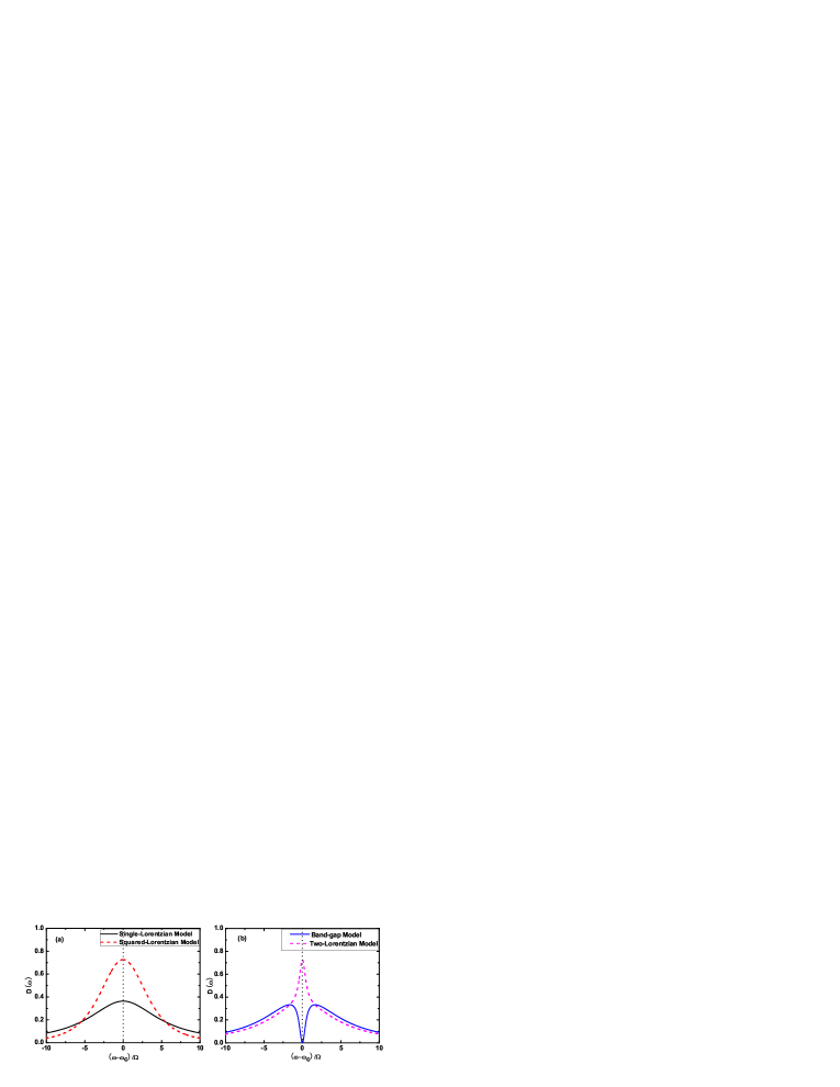
Figure 3: The density of the spectrum $D(\omega)$ as a function of the dimensionless quantity $(\omega-\omega_{c})$ in the weak-coupling regime. (a) for the single-Lorentzian and squared-Lorentzian as the environmental models, with $\Gamma=11\Omega$; (b) for the two-Lorentzian and band-gap as the environmental models, with $\Gamma_{1}=11\Omega$, $\Gamma_{2}=\Omega$.

In this paper, we also understand the influences of different environments on the atomic QD in the strong coupling regimes which satisfy $\Gamma=0.11\Omega$ in the single-Lorentzian environment and squared-Lorentzian environment, and $\Gamma_{1}=0.11\Omega$, $\Gamma_{2}=0.01\Omega$ in the two-Lorentzian environment and band-gap environment. In Fig. $4$, we acquire that the periodically oscillating decay speed of the atomic QD in the squared-Lorentzian (two-Lorentzian) environment is slower than in the single-Lorentzian (band-gap) environment, either under the atom-pseudomode near resonant or far off-resonant condition. That is to say, in the strong coupling regime the QD is more robust in the squared-Lorentzian (two-Lorentzian) environment than in the single-Lorentzian (band-gap) environment. In what follows, we will give a simple interpretation for why this finding in the strong regime is different from the results in the weak coupling regime. First, taking the spectrum density function $D(\omega)$ of the above four environmental models into account in the strong regime, we note that the discrepancy among them is very minor, as shown in Fig. $5$. So from the spectrum density function to give a construction is not feasible.

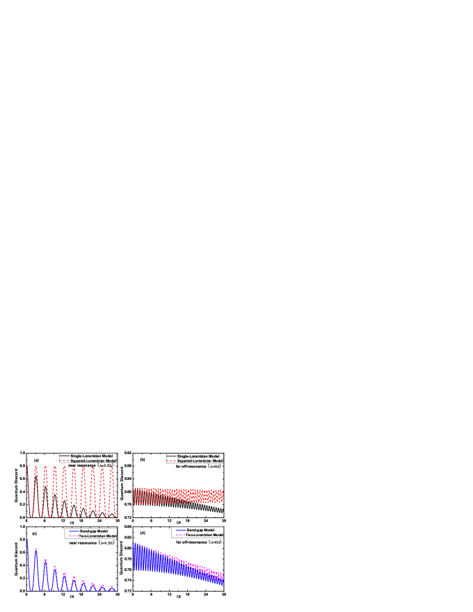
Figure 4: (Color online) Time evolution of the atomic QD as a function of the dimensionless quantity ${\Omega}t$ under the atom-pseudomode near resonance regime and far off-resonance regime, with $\theta=\pi/3$. (a) and (b) the single-Lorentzian and squared-Lorentzian as the environmental models, with $\Gamma=0.11\Omega$; (c) and (d) the two-Lorentzian and band-gap as the environmental models, with $\Gamma_{1}=0.11\Omega$, $\Gamma_{2}=0.01\Omega$.

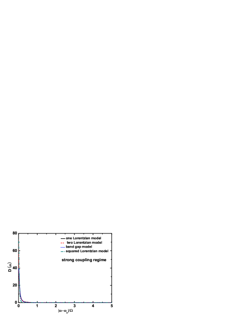
Figure 5: The density of the spectrum $D(\omega)$ as a function of the dimensionless quantity $(\omega-\omega_{c})$ in the strong-coupling regime, for the single-Lorentzian and squared-Lorentzian as the environmental models, with $\Gamma=0.11\Omega$; and for the two-Lorentzian and band-gap as the environmental models, with $\Gamma_{1}=0.11\Omega$, $\Gamma_{2}=0.01\Omega$.

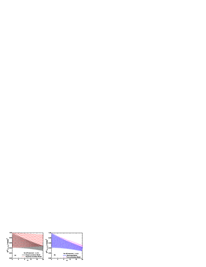
Figure 6: (Color online) Time evolution of the trace distance $D^{S}(\rho_{1},\rho_{2})$ as a function of the dimensionless quantity ${\Omega}t$ under the far off-resonance regime, with $\rho_{1}(0)=|e\rangle{\langle}e|$ and $\rho_{2}(0)=|g\rangle{\langle}g|$. (a) for the single-Lorentzian and squared-Lorentzian as the environmental models, with $\Gamma=0.11\Omega$; (b) for the two-Lorentzian and band-gap as the environmental models, with $\Gamma_{1}=0.11\Omega$, $\Gamma_{2}=0.01\Omega$.

However, according to the previous works [26-28], we know that there exists the non-Markovianity of environment in the strong coupling regime, and the non-Markovian effect of environment can play an important role on the dynamics of the qubits system. Therefore, we will show the degree of the non-Markovian behavior of the dynamics processes in these different environmental models. In Ref. [26], Breuer $et$ $al.$ suggest definition a measure $N(\Phi)$ for the non-Markovianity of the quantum process $\Phi(t)$ by means of the relation $N(\Phi)=\max_{\rho_{1,2}(0)}\sum_{i}[D(\rho_{1}(b_{i}),\rho_{2}(b_{i}))-D(\rho_{1}(a_{i}),\rho_{2}(a_{i}))]$. To calculate this quantity one first determines the total growth of the trace distance over each time interval $(a_{i},b_{i})$ and sums up the contributions of all intervals. Then $N(\Phi)$ can be obtained by determining the maximum over all pairs of initial states. Taking the far off-resonance as an example, the analytical expression of the trace distance in the atom-environment dynamics process is $D^{S}(\rho_{1},\rho_{2})=|b(t)|^{2}$, here with $b(t)$ represents the amplitude damping of the excited state $|e\rangle$, and the pair of initial states $\rho_{1}(0)=|e\rangle{\langle}e|$ and $\rho_{2}(0)=|g\rangle{\langle}g|$ which optimize the total increase of $D^{S}(\rho_{1},\rho_{2})$. Thus, we can qualitatively and intuitively compare the non-Markovianity due to the different environment models by the time evolution of the trace distance. Fig. $6$ shows the trace distance $D^{S}(\rho_{1},\rho_{2})$ as a function of ${\Omega}t$ for $\Delta=8\Omega$, namely, the far off-resonance regime. It is very interesting to note that the amplitudes of $D^{S}(\rho_{1},\rho_{2})$ caused by squared-Lorentzian (two-Lorentzian) environment are much wider than those caused by the single-Lorentzian (band-gap) environment. In other words, the non-Markovianity of the squared-Lorentzian (two-Lorentzian) environment is much stronger than the single-Lorentzian (band-gap) environment. This finding leads to a clear interpretation for the result obtained by Fig. $4$: the atomic QD in the strong coupling regime is determined by the different degree of environmental non-Markovianity, and is independent of the spectrum density function $D(\omega)$.
In conclusion, we have studied the quantum correlation dynamics in the different decoherence environments, and considered a two-atom system interacting with two local, independent environments, modeling several common noise sources: the single-Lorentzian model, the squared-Lorentzian model, the two-Lorentzian model and band-gap model. For the weak coupling regime, it is clear to realize that the atomic QD in the single-Lorentzian (band-gap) environment is more robust than in the squared-Lorentzian (two-Lorentzian) environment under the resonant and near resonant conditions. But for the far off-resonant condition the opposite result shows that the atomic QD in the single-Lorentzian (band-gap) environment decreases much more faster than in the squared-Lorentzian (two-Lorentzian) environment. However, for the strong coupling regime, the atomic QD is more robust in the squared-Lorentzian (two-Lorentzian) environment than in the single-Lorentzian (band-gap) environment, either under the atom-pseudomode near resonant or far off-resonant condition. Finally we note that we study here only the two-atom system interacting with their independent environments. An important future investigation will be the study of the effects of these different environmental models on the dynamics of the two-atom system under a common environment, where quantum correlations can be created in the system through nonlocal interactions mediated by the environment.

IV Acknowledgments

This work is supported by National Natural Science Foundation of China under Grant Nos. 61178012 and 10947006, the Specialized Research Fund for the Doctoral Program of Higher Education under Grant No. 20093705110001 and the Research Funds from Qufu Normal University under Grant No. XJ201013.