Opto- and electro-mechanical entanglement improved by modulation

Abstract

One of the main milestones in the study of opto- and electro-mechanical systems is to certify entanglement between a mechanical resonator and an optical or microwave mode of a cavity field. In this work, we show how a suitable time-periodic modulation can help to achieve large degrees of entanglement, building upon the framework introduced in [Phys. Rev. Lett. 103, 213603 (2009)]. It is demonstrated that with suitable driving, the maximum degree of entanglement can be significantly enhanced, in a way exhibiting a non-trivial dependence on the specifics of the modulation. Such time-dependent driving might help experimentally achieving entangled mechanical systems also in situations when quantum correlations are otherwise suppressed by thermal noise.

I Introduction

Opto-mechanical Opto1 ; Opto2 ; Opto3 ; Opto4 ; Opto5 ; KippenCold ; AspelCold and electro-mechanical systems EM0 ; EM1 ; EM2 ; EM3 ; EMCold ; SB are promising candidates for realizing architectures exhibiting quantum behavior in macroscopic structures. Once the quantum regime is reached, exciting applications in quantum technologies such as realizing precise force sensors are conceivable Schwab ; Marquardt . One of the requirements to render such an approach feasible, needless to say, is to be able to certify that a mechanical degree of freedom is deeply in the quantum regime Marquardt ; QR1 ; QR2 ; QR3 ; QR4 . The detection of entanglement arguably constitutes the ultimate benchmark in this respect. While effective ground state cooling has indeed been experimentally closely approached EMCold ; KippenCold and achieved SB ; EM0 ; AspelCold , the detection of entanglement is still awaiting.

In this work, we emphasize that a mere suitable time-modulation of the driving field may significantly help to achieve entanglement between a mechanical mode and a radiation mode of the system. We extend the idea of Ref. Ours , putting emphasis on the improvement of entanglement by means of suitable modulations Ours ; Clerk ; Woolley . The method used here is not a direct modulation of the frequencies of the two modes (parametric amplification), but the system is instead externally driven with a modulated field. This time dependence of the driving indirectly affects the effective radiation pressure coupling between the two modes and generates non-trivial entanglement resonances. In this way, with the appropriate choice of the modulation pattern, large degrees of two-mode squeezing can be reached.

II Modulated opto- and electro-mechanical systems

We consider the simplest scenario of a mechanical resonator of frequency $\omega_{m}$ coupled to a single mode of the electromagnetic field of frequency $\omega_{a}$. This radiation field could be an optical mode of a Fabry-Perot cavity Opto1 ; Opto2 ; Opto3 ; Opto4 ; Opto5 ; SidebandCooling ; KippenCold ; AspelCold ; QR2 ; QR3 or a microwave mode of a superconductive circuit EM0 ; EM3 ; EMCold ; EMtheory . It can be shown that the Hamiltonians associated to this two experimental settings are formally equivalent QR3 ; EMtheory and therefore the theory that we are going to introduce is general enough to describe both types of systems.

We assume that the radiation mode is driven by a coherent field with a time dependent amplitude $E(t)$ and frequency $\omega_{l}$. The particular choice of the time dependence is left unspecified but we impose the structure of a periodic modulation such that $E(t+\tau)=E(t)$ for some $\tau>0$ of the order of $\omega_{m}^{-1}$. In this sense, the driving regime that we are going to study is intermediate between the two opposite extremes of constant amplitude and short pulses. The Hamiltonian of the system is

$$H=\hbar\omega_{a}a^{\dagger}a+\frac{1}{2}\hbar\omega_{m}(p^{2}+q^{2})-\hbar ga^{\dagger}aq$$

$$+i\hbar[E(t)e^{-i\omega_{l}t}a^{\dagger}-E^{*}(t)e^{i\omega_{l}t}a],$$ (1)

where the mechanical mode is described in terms of dimensionless position and momentum operators satisfying $[q,p]=i$, while the radiation mode is captured by creation and annihilation operators obeying the bosonic commutation rule $[a,a^{\dagger}]=1$. The two modes interact via a radiation pressure potential with a strength given by the coupling parameter $g$.

In addition to this coherent dynamics, the mechanical mode will be unavoidably damped at a rate $\gamma_{m}$, while the optical/microwave mode will decay at a rate $\kappa$. These dissipative processes and the associated fluctuations can be taken into account in the Heisenberg picture by the following set of quantum Langevin equations QR1 ; QR2 ; QR3 ; EMtheory ,

$$\dot{q} = \omega_{m}p,$$ (2)

$$\dot{p} = -\omega_{m}q-\gamma_{m}p+ga^{{\dagger}}a+\xi,$$

$$\dot{a} = -(\kappa+i\Delta)a+igaq+E(t)+\sqrt{2\kappa}a^{\rm in}.$$

In this set of equations a convenient rotating frame has be chosen $a\mapsto ae^{-i\omega_{l}t}$, such that the detuning parameter is $\Delta=\omega_{a}-\omega_{l}$. The operators $\xi$ and $a^{\rm in}$ represent the mechanical and optical bath operators respectively, and their correlation functions are well approximated by delta functions

$$\langle\xi(t)\xi(t^{\prime})+\xi(t^{\prime})\xi(t)\rangle/2 = \gamma_{m}(2n_{m}+1)\delta(t-t^{\prime}),$$ (3)

$$\langle a^{\rm in}(t)a^{\rm in{\dagger}}(t^{\prime})\rangle = (n_{a}+1)\delta(t-t^{\prime}),$$

$$\langle a^{\rm in{\dagger}}(t)a^{\rm in}(t^{\prime})\rangle = n_{a}\delta(t-t^{\prime}),$$

where $n_{x}=(\text{exp}{({\hbar\omega_{x}}/({k_{B}T}))}-1)^{-1}$, is the bosonic mean occupation number at temperature $T$.

III Classical periodic orbits: first moments

We are interested in the coherent strong driving regime when $\langle a\rangle\gg 1$. In this limit, the semiclassical approximations $\langle a^{{\dagger}}a\rangle\simeq|\langle a\rangle|^{2}$ and $\langle aq\rangle\simeq\langle a\rangle\langle q\rangle$ are good approximations. Within this approximation, one can average both sides of Eq. (2) and get a differential equation for the first moments of the canonical coordinates

$$\langle\dot{q}\rangle = \omega_{m}\langle p\rangle,$$ (4)

$$\langle\dot{p}\rangle = -\omega_{m}\langle q\rangle-\gamma_{m}\langle p\rangle+g|\langle a\rangle|^{2},$$

$$\langle\dot{a}\rangle = -(\kappa+i\Delta)\langle a\rangle+ig\langle a\rangle\langle q\rangle+E(t).$$

Far away from the well known opto- and electro-mechanical instabilities, asymptotic $\tau$-periodic solutions can be used as ansatz for Eqs. (4) (see the Appendix for a more detailed analysis). These solutions represent periodic orbits in phase space and are usually called limit cycles. These cycles are induced by the modulation and should not be confused with the limit cycles emerging in the strong driving regime due to the non-linearity of the system. Because of the asymptotic periodicity of the solutions, one can define the fundamental modulation frequency as $\Omega=2\pi/\tau$, such that each periodic solution can be expanded in the following Fourier series

$$\langle O(t)\rangle = \sum_{n=-\infty}^{\infty}O_{n}e^{in\Omega t},\quad O=q,p,a.$$ (5)

The Fourier coefficients $\{O_{n}\}$ appearing in Eq. (5) can be analytically estimated as shown in Appendix and they completely characterize the classical asymptotic dynamics of the system.

Finally we notice that the classical evolution of the dynamical variables will shift the detuning to the effective value of $\tilde{\Delta}(t)=\Delta-g\langle q(t)\rangle$. For the same reason, it is also convenient to introduce an effective coupling constant defined as

$$\tilde{g}(t)=ig\langle a(t)\rangle/\sqrt{2}.$$ (6)

IV Quantum correlations: second moments

The classical limit cycles are given by the asymptotic solutions of Eqs. (4). In order to capture the quantum fluctuations around the classical orbits, we introduce a column vector of new quadrature operators $u=[\delta q,\delta p,\delta x,\delta y]^{T}$ defined as:

$$\delta q = q-\langle q(t)\rangle,$$ (7)

$$\delta p = p-\langle p(t)\rangle,$$

$$\delta x = \left[(a-\langle a(t)\rangle)+(a-\langle a(t)\rangle)^{\dagger}\right]/\sqrt{2},$$

$$\delta y = -i\left[(a-\langle a(t)\rangle)-(a-\langle a(t)\rangle)^{\dagger}\right]/\sqrt{2}.$$

This set of canonical coordinates can be viewed as describing a time-dependent reference frame co-moving with the classical orbits. The corresponding vector of noise operators will be

$$n=[0,\xi,(a^{\rm in}+a^{\rm in{\dagger}})/\sqrt{2},-i(a^{\rm in}-a^{\rm in{\dagger}})/\sqrt{2}]^{T}.$$ (8)

Since we are in the limit in which classical orbits emerge ($\langle a\rangle\gg 1$), it is a reasonable approximation to express the previous set of Langevin equations (2) in terms of the new fluctuation operators (7) and neglect all quadratic powers of them. The resulting linearized system can be written as a matrix equation Ours ,

$$\dot{u}=A(t)u+n(t),$$ (9)

where,

$$A(t) = \left[\begin{array}[]{cccc}0&\omega_{m}&0&0\\ -\omega_{m}&-\gamma_{m}&\Re\tilde{g}(t)&\Im\tilde{g}(t)\\ -\Im\tilde{g}(t)&0&-\kappa&\tilde{\Delta}(t)\\ \Re\tilde{g}(t)&0&-\tilde{\Delta}(t)&-\kappa\end{array}\right]$$ (14)

is a real time-dependent matrix.

If the system is stable, and as long as the linearization is valid, the quantum state of the system will converge to a Gaussian state with time dependent first and second moments. The first moments of the state correspond to the classical limit cycles introduced in the previous section. The second moments can be expressed in terms of the covariance matrix $V(t)$ with entries

$$V_{k,l}(t)=\langle u_{k}(t)u_{l}^{\dagger}(t)+u_{l}^{\dagger}(t)u_{k}(t)\rangle/2.$$ (15)

One can also define a diffusion matrix $D$ as

$$\delta(t-t^{\prime})D_{k,l}=\langle n_{k}(t)n_{l}^{\dagger}(t^{\prime})+n_{l}^{\dagger}(t^{\prime})n_{k}(t)\rangle/2,$$ (16)

which, from the properties of the bath operators (3), is diagonal and equal to

$$D={\rm diag}[0,\gamma(2n_{m}+1),\kappa(2n_{a}+1),\kappa(2n_{a}+1)].$$ (17)

From Eqs. (9) and (16), one can easily derive a linear differential equation for the correlation matrix,

$$\frac{d}{dt}V(t)=A(t)V(t)+V(t)A^{T}(t)+D.$$ (18)

Since the first and the second moments are specified, Eqs. (4) and (18) provide a complete description of the asymptotic dynamics of the system. Apart from the linearization around classical cycles, no further approximation has been done: Neither a weak coupling, adiabatic or rotating-wave approximation. Numerical solutions of both equations (4) and (18) can be straightforwardly found. These solutions will be used to calculate the exact amount opto- and electro-mechanical entanglement present in the system.

The asymptotic periodicity of the classical solutions (Eq. (5)) implies that, in the long time limit, $A(t+\tau)=A(t)$. This means that Eq. (18) is a linear differential equation with periodic coefficients and then all the machinery of Floquet theory is in principle applicable. Here, however, since we are only interested on asymptotic solutions, we are not going to study all the Floquet exponents of the system. The only property that we need is that, in the long time limit, stable solutions will acquire the same periodicity of the coefficients:

$$V(t+\tau)=V(t).$$ (19)

This is a simple corollary of Floquet’s theorem. In the subsequent sections we will apply the previous theory to some particular experimental setting and show how a simple modulation of the driving field can significantly improve the amount of opto- and electro-mechanical entanglement.

V Entanglement resonances

In this section we are going to study what kind of amplitude modulation is optimal for generating entanglement between the radiation and mechanical modes. As a measure of entanglement we use the logarithmic negativity $E_{N}$ which, since the state is Gaussian, can be easily computed directly from the correlation matrix $V(t)$ Neg1 ; Neg2 ; Neg3 . We have also seen that the correlation matrix is, in the long time limit, $\tau$-periodic. This suggests that it is sufficient to study the variation of entanglement in a finite interval of time $[t,t+\tau]$ for large times $t$. One can then define the maximum amount of achievable entanglement as

$$\hat{E}_{N}=\lim_{t\rightarrow\infty}\max_{h\in[t,t+\tau]}E_{N}(h).$$ (20)

This will be the quantity that we are going to optimize.

We first study a very simple set of parameters (see caption of Figure 1) in order to understand what the optimal choice is for the modulation frequency. For this purpose we impose the effective coupling to have this simple structure

$$\tilde{g}(t)=\tilde{g}_{0}+\tilde{g}_{\Omega}\;e^{-i\Omega t},$$ (21)

where $\tilde{g}_{0}$ is associated to the main driving field with detuning $\Delta$, while $\tilde{g}_{\Omega}$ is the amplitude of a further sideband shifted by a frequency $\Omega$ from the main carrier. Without loss of generality we will assume $\tilde{g}_{0}$ and $\tilde{g}_{\Omega}$ to be positive reals. This kind of driving is a natural one and has been chosen for reasons that will become clear later. From now on we set the detuning of the carrier frequency to be equal to the mechanical frequency $\Delta=\omega_{m}$. This choice of the detuning corresponds to the well known sideband cooling setting SidebandCooling ; QR1 and it has been shown to be also optimal for maximizing opto-mechanical entanglement with a non-modulated driving QR3 . Fig. 1 shows the maximum entanglement $\hat{E}_{N}$ between the mechanical and the radiation modes as a function of the modulation frequency $\Omega$ and for different values of the driving amplitude $\tilde{g}_{0}$. This maximum degree of entanglement has been calculated for $t>200/\kappa$ when the system has well reached its periodic steady state.

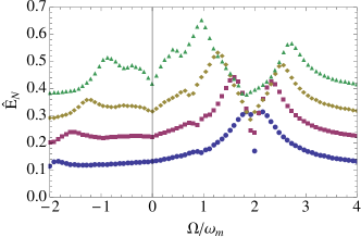
Figure 1: Maximum entanglement $\hat{E}_{N}$ as a function of the modulation frequency $\Omega$ and for different values of the driving strength $\tilde{g}_{0}$. The chosen parameters in units of $\omega_{m}$ are: $\kappa=0.2$, $\gamma_{m}=10^{-6}$, $\tilde{\Delta}=1$, $n_{m}=n_{a}=0$, $\tilde{g}_{\Omega}=0.1$, $\tilde{g}_{0}=$ $0.2$ (circles), $0.4$ (squares), $0.6$ (diamonds), $0.8$ (triangles).

We observe that in Fig. 1 there are two main resonant peaks at the modulation frequencies

$$\Omega\simeq 2\omega_{m}\pm\tilde{g}_{0}.$$ (22)

We will now provide some intuition why one should expect the main resonances at the locations where they are observed. First assume that $\tilde{g}_{0}=0$. Then, for $\Delta=\omega_{m}$, the linearized Hamiltonian in the interaction picture is

$$H_{\rm int} = -\hbar\tilde{g}_{\Omega}\left(e^{i(\omega_{m}-\Omega)}\delta a^{\dagger}+e^{-i(\omega_{m}-\Omega)}\delta a\right)$$ (23)

$$\left(e^{i\omega_{m}}\delta b^{\dagger}+\delta be^{-i\omega_{m}}\right)/2,$$

where the bosonic operators are defined as $\delta a=(\delta x+i\delta y)/\sqrt{2}$, $\delta b=(\delta q+i\delta p)/\sqrt{2}$. From Eq. (23), it is clear that for $\Omega=2\omega_{m}$, neglecting all rotating terms, we get the well known two-mode squeezing generator

$$H_{\rm int} \simeq -\hbar\tilde{g}_{\Omega}\left(\delta a^{\dagger}\delta b^{\dagger}+\delta a\delta b\right)/2.$$ (24)

So, in the case of $\tilde{g}_{0}=0$, a modulation of $\Omega=2\omega_{m}$ would be the most reasonable choice in order to generate entanglement. However, this regime is well known to be highly unstable and, in practice, it cannot be used for preparing entangled steady states EMtheory .

This is why we need to consider a modulated coupling of the form given in Eq. (21) – or a similar type of modulation sharing these features. We now allow for $\tilde{g}_{0}$ being different from zero, giving rise to a situation which can be assessed in a very similar way as above (only that the rotation terms will take a more involved form). The main amplitude $\tilde{g}_{0}$ then takes the role of cooling and stabilizing the system while the modulation amplitude $\tilde{g}_{\Omega}$ is used to generate entanglement. At the same time however, as shown in Refs. ModeSplitting ; Opto4 , for $\tilde{g}_{0}>\kappa/\sqrt{2}$ the system hybridizes in two normal modes of frequencies

$$\omega_{\pm}\simeq\omega_{m}\pm\tilde{g}_{0}/2.$$ (25)

As a consequence, this will affect the modulation frequency $\Omega$ that one has to choose in order to achieve the two-mode squeezing interaction given in Eq. (24). This is the reason for the presence of two resonant peaks in Fig. 1 and for the resonance condition given in Eq. (22).

Note also that the choices of modulations that give rise to the optimal local single-mode squeezing Ours of the mechanical mode and the degree of entanglement are not identical. This is rooted in the “monogamous nature” of squeezing: For a fixed spectrum of the covariance matrix, one can either have large local or two-mode squeezing. This effect is observed when considering the modulation frequencies that achieve maximum single- and two-mode squeezing.

We finally observe that the height of the two peaks, due to the cavity filtering, is not equal: the first resonance at $\Omega=2\omega_{m}-\tilde{g}_{0}$ is better for the amount of steady state entanglement. One could also ask what the behavior of entanglement is when we change the amplitude of the modulation. Fig. 2 shows the amount of entanglement $\hat{E}_{N}$ as a function of $\tilde{g}_{\Omega}$ and for different choices of $\tilde{g}_{0}$. We observe that entanglement is monotonically increasing in $\tilde{g}_{\Omega}$ up to a threshold where the system becomes unstable.

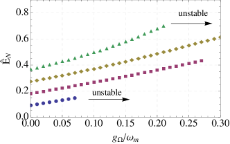
Figure 2: Maximum entanglement $\hat{E}_{N}$ as a function of the modulation amplitude $\tilde{g}_{\Omega}$ and for different values of the driving strength $\tilde{g}_{0}$. The chosen parameters in units of $\omega_{m}$ are: $\kappa=0.2,\gamma_{m}=10^{-6}$, $\tilde{\Delta}=1$, $n_{m}=n_{a}=0$, $\Omega=2\omega_{m}-\tilde{g}_{0}$, $\tilde{g}_{0}=0.2$ (circles), $0.4$ (squares), $0.6$ (diamonds), $0.8$ (triangles).

VI Opto- and electro-mechanical entanglement in realistic settings

We have seen that an effective coupling of the form $\tilde{g}(t)=\tilde{g}_{0}+\tilde{g}_{\Omega}\;e^{-i(2\omega_{m}-\tilde{g}_{0})t}$ is optimal for the generation of entanglement within the considered class of drivings. However, the parameter $\tilde{g}(t)$ depends on the average amplitude $\langle a(t)\rangle$ and assuming such a simple structure may seem somewhat artificial. In this section, we show how the desired time-dependent coupling can indirectly result from the classical limit cycles of the system (see insets of Figs. 3 and 4) and we also take into account the effect of a temperature of the order of $T\simeq 100$ mK. The natural “educated guess” for the structure of the driving field will be

$$E(t)=E_{0}+E_{\Omega}Ee^{-i(2\omega_{m}-\tilde{g}_{0})t}.$$ (26)

For the choice of the other parameters, we focus on two set of parameters corresponding to two completely different systems: an optical cavity with a moving mirror and a superconducting wave guide coupled to a mechanical resonator. The parameters are chosen according to realistic experimental settings, see, e.g., Ref. Opto4 (opto-mechanical system) and Ref. EM0 (electro-mechanical system). Fig. 3 and Fig. 4 show that, in both experimental scenarios, entanglement can significantly be increased by an appropriate modulation of the driving field.

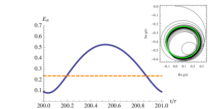
Figure 3: (Optical cavity). The degree of entanglement, measured in terms of the logarithmic negativity, as a function of time. The full line refers to a modulated driving ($\Omega=1.4\omega_{m}$) while the dotted line corresponds to a non-modulated driving ($\Omega=0$). The chosen parameters in units of $\omega_{m}$ are: $\kappa=0.2$, $\gamma_{m}=10^{-6}$, $\Delta=1$, $n_{m}=2\times 10^{3}$, $n_{a}=0$, $g_{0}=4\times 10^{-6}$, $E_{0}=7\times 10^{4}$, $E_{\Omega}=2.5\times 10^{4}$. The inset shows the trajectory of the effective coupling $\tilde{g}(t)=\sqrt{2}g\langle a(t)\rangle$ in the complex plane due to the time evolution of the optical amplitude. The phase space orbit (black line) is numerically simulated from Eq. (4), while the limit cycle (green line) is an analytical approximation (see Appendix for more details).

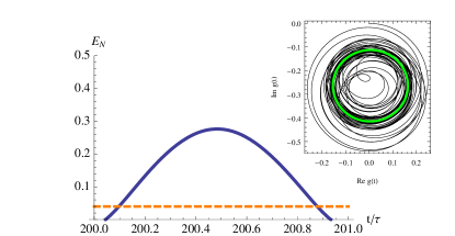
Figure 4: (Microwave cavity). Entanglement log-negativity as a function of time. The full line refers to a modulated driving ($\Omega=1.3\omega_{m}$) while the dotted line corresponds to a non-modulated driving ($\Omega=0$). The chosen parameters in units of $\omega_{m}$ are: $\kappa=0.02$, $\gamma_{m}=3\times 10^{-6}$, $\Delta=1$, $n_{m}=200$, $n_{a}=0.03$, $g_{0}=2\times 10^{-5}$, $E_{0}=9\times 10^{3}$, $E_{\Omega}=1.3\times 10^{3}$. The inset depicts the trajectory of the effective coupling $\tilde{g}(t)=\sqrt{2}g\langle a(t)\rangle$ in the complex plane due to the time evolution of the microwave amplitude. The phase space orbit (black line) is numerically simulated from Eq. (4), while the limit cycle (green line) is an analytical approximation (see Appendix for more details).

VII Summary

In this work, we have shown how time-modulation can significantly enhance the maximum degree of entanglement. Triggered by the time-modulated driving, the mode of the electromechanical field as well as the mechanical mode start “rotating around each other” in a complex fashion, giving rise to increased degrees of entanglement. The dependence on the frequencies of the additional modulation is intricate, with resonances highly improving the amount of entanglement that can be reached. The ideas presented here could be particularly beneficial to prepare systems in entangled states in the first place, in scenarios where the parameters are such that the states prepared are close to the boundary to entangled states, but where this boundary is otherwise not yet quite reachable with present technology. At the same time, such ideas are expected to be useful in metrological applications whenever high degrees of entanglement are needed.

VIII Appendix

In this appendix we derive analytical formulas for the asymptotic solutions of the classical system of dynamical equations (4). A crucial assumption for the following procedure is that it is possible to expand the solutions in powers of the the coupling constant $g_{0}$

$$\langle O\rangle(t)=\sum_{j=0}^{\infty}O_{j}(t)g_{0}^{j},$$ (27)

where $O=a,p,q$. This is justified only if the system is far away from multi-stabilities and the radiation pressure coupling can be treated in a perturbative way. A very important feature of the set of equations (4) is that they contain only two non linear terms and those terms are proportional to the coupling parameter $g_{0}$. This implies that, if we use the ansatz (27), each function $O_{j}$ will be a solution of linear differential equation with time dependent parameters depending on the previous solution $O_{j-1}(t)$. Since $E(t)=E(t+\tau)$, from a recursive application of Floquet’s theorem, follows that stable solutions will converge to periodic limit cycles having the same periodicity of the driving: $\langle O(t)\rangle=\langle O(t+\tau)\rangle$. One can exploit this property and perform a double expansion in powers of $g_{0}$ and in terms of Fourier components

$$\langle O\rangle(t)=\sum_{j=0}^{\infty}\sum_{n=-\infty}^{\infty}O_{n,j}e^{in\Omega t}g_{0}^{j},$$ (28)

where $n$ are integers and $\Omega=2\pi/\tau$. A similar Fourier series can be written for the periodic driving field,

$$E(t)=\sum_{n=-\infty}^{\infty}E_{n}e^{in\Omega t}.$$ (29)

The coefficients $O_{n,j}$ can be found by direct substitution in Eq. (4). They are completely determined by the following set of recursive relations:

$$q_{n,0}=p_{n,0}=0,\qquad a_{n,0}=\frac{E_{-n}}{\kappa+i(\Delta_{0}+n\Omega)},$$ (30)

corresponding to the $0$-order perturbation with respect to $G_{0}$, and

$$p_{n,j} = \frac{in\Omega}{\omega_{m}}q_{n,j},$$ (31)

$$q_{n,j} = \omega_{m}\sum_{k=0}^{j-1}\sum_{m=-\infty}^{\infty}\frac{a_{m,k}^{*}\;a_{n+m,j-k-1}}{\omega_{m}^{2}-n\Omega^{2}+i\gamma_{m}n\Omega},$$ (32)

$$a_{n,j} = i\sum_{k=0}^{j-1}\sum_{m=-\infty}^{\infty}\frac{a_{m,k}q_{n-m,j-k-1}}{\kappa+i(\Delta_{0}+n\Omega)},$$ (33)

giving all the $j$-order coefficients in a recursive way. For all the examples analyzed in this paper we truncated the analytical solutions up to $j\leq 3$ and $|n|\leq 2$. This level of approximation is already high enough to well reproduce the exact numerical solutions.

IX Acknowledgements

We would like to thank the EU (MINOS, COMPAS, QESSENCE) and the BMBF (QuOReP) for support.

References

- (1) S. Gigan, H. R. Böhm, M. Paternostro, F. Blaser, G. Langer, J. B. Hertzberg, K. Schwab, D. Baeuerle, M. Aspelmeyer, and A. Zeilinger, Nature 444, 67 (2006).
- (2) O. Arcizet, P.-F. Cohadon, T. Briant, M. Pinard, and A. Heidmann, Nature 444, 71 (2006).
- (3) D. Kleckner and D. Bouwmeester, Nature 444, 75 (2006).
- (4) A. Schliesser, P. Del Haye, N. Nooshi, K. J. Vahala, and T. J. Kippenberg, Phys. Rev. Lett. 97, 243905 (2006).
- (5) S. Gröblacher, K. Hammerer, M. R. Vanner, and M. Aspelmeyer, Nature 460, 724 (2009).
- (6) R. Riviere, S. Deleglise, S. Weis, E. Gavartin, O. Arcizet, A. Schliesser, T. J. Kippenberg, Phys. Rev. A 83, 063835 (2011).
- (7) J. Chan, T. P. Mayer Alegre, A. H. Safavi-Naeini, J. T. Hill, A. Krause, S. Groeblacher, M. Aspelmeyer, and O. Painter, Nature 478, 89 (2011).
- (8) J. D. Teufel, J. W. Harlow, C. A. Regal, and K. W. Lehnert, Phys. Rev. Lett. 101, 197203 (2008).
- (9) J. D. Teufel, T. Donner, D. Li, J. H. Harlow, M. S. Allman, K. Cicak, A. J. Sirois, J. D. Whittaker, K. W. Lehnert, and R. W. Simmonds, Nature 475, 359 (2011).
- (10) T. Rocheleau, T. Ndukum, C. Macklin, J. B. Hertzberg, A. A. Clerk, and K. C. Schwab, Nature 463, 72 (2010).
- (11) M. D. LaHaye, O. Buu, B. Camarota, and K. C. Schwab, Science 304, 74 (2004).
- (12) R. G. Knobel and A. N. Cleland, Nature 424, 291 (2003).
- (13) A. D. O Connell, M. Hofheinz, M. Ansmann, R. C. Bialczak, M. Lenander, E. Lucero, M. Neeley, D. Sank, H. Wang, M. Weides, J. Wenner, J. M. Martinis, and A. N. Cleland, Nature 464, 697 (2010).
- (14) D. Vitali, P. Tombesi, M. J. Woolley, A. C. Doherty, and G. J. Milburn, Phys. Rev. A 76, 042336 (2007).
- (15) K. C. Schwab and M. L Roukes, Physics Today 58, 36 (2005).
- (16) F. Marquardt and S. M. Girvin, Physics 2, 40 (2009).
- (17) M. Aspelmeyer, Nature 464, 685 (2010).
- (18) M. Paternostro, D. Vitali, S. Gigan, M. S. Kim, C. Brukner, J. Eisert, and M. Aspelmeyer, Phys. Rev. Lett. 99, 250401 (2007).
- (19) D. Vitali, S. Gigan, A. Ferreira, H. R. Böhm, P. Tombesi, A. Guerreiro, V. Vedral, A. Zeilinger, and M. Aspelmeyer, Phys. Rev. Lett. 98, 030405 (2007).
- (20) J. Eisert, M. B. Plenio, S. Bose, and J. Hartley, Phys. Rev. Lett. 93, 190402 (2004).
- (21) A. Mari and J. Eisert, Phys. Rev. Lett. 103, 213603 (2009).
- (22) M. J. Woolley, A. C. Doherty, G. J. Milburn, and K. C. Schwab, Phys. Rev. A 78, 062303 (2008).
- (23) A. A. Clerk, F. Marquardt, and K. Jacobs, New J. Phys. 10, 095010 (2008).
- (24) F. Marquardt, J. P. Chen, A. A. Clerk, and S. M. Girvin Phys. Rev. Lett. 99, 093902 (2007).
- (25) J. M. Dobrindt, I. Wilson-Rae, and T. J. Kippenberg Phys. Rev. Lett. 101, 263602 (2008).
- (26) J. Eisert, PhD thesis (Potsdam, February 2001).
- (27) G. Vidal and R. F. Werner, Phys. Rev. A 65, 032314 (2002).
- (28) M. B. Plenio, Phys. Rev. Lett. 95, 090503 (2005).