Atom-mediated effective interactions between modes of a bimodal cavity

Abstract

We show a procedure for engineering effective interactions between two modes in a bimodal cavity. Our system consists of one or more two-level atoms, excited by a classical field, interacting with both modes. The two effective Hamiltonians have a similar form of a beam-splitter and quadratic beam-splitter interactions, respectively. We also demonstrate that the nonlinear Hamiltonian can be used to prepare an entangled coherent state, also known as multidimensional entangled coherent state, which has been pointed out as an important entanglement resource. We show that the nonlinear interaction parameter can be enhanced considering $N$ independent atoms trapped inside a high-finesse optical cavity.

I Introduction

Cavity Quantum Electrodynamics (CQED) is an ideal scenario for research on fundamentals of quantum theory and quantum information. Achievements on both, the construction of high quality cavities and control of atom-field interactions, are associated with the use of the entanglement properties for the successful generation of quantum states of light, such as Einstein-Podolski-Rosen (EPR), Schrödinger cat and Fock states Raimond et al. (2001). An important consequence of the high experimental control in CQED was the successful reconstruction of quantum states of light prepared inside a high quality cavity Bertet et al. (2002); Delèglise et al. (2008). This procedure allows, for example, the observation of decoherence process of a Schrödinger cat-like state, through the analysis of snapshots of the Wigner function Wigner (1932); Hillery et al. (1984). The same setup was also used to reconstruct the Wigner function of Fock states with more than one photon Delèglise et al. (2008). Recently, CQED setups has been used in order to study three-photon correlations Koch et al. (2011), the apparition of electromagnetically induced transparency using Rubidium Mücke et al. (2010) and Cesium Kampschulte et al. (2010) single atoms and quantum jumps Reick et al. (2010); Khudaverdyan et al. (2009).

A particular CQED experimental setup could include a bimodal cavity. In this kind of device, two bosonic modes with different polarizations are prepared inside the cavity Rauschenbeutel et al. (2001). In the context of quantum information theory, a bimodal cavity is interesting because the additional mode acts as a third photonic qubit (besides the atom and the first cavity mode qubits), opening new possibilities for implementation of quantum information protocols Messina et al. (2003). Potential applications of bimodal cavities have been analyzed in some recent works. Those include the implementation of quantum logic gates Dong et al. (2009) and generation of entangled states Gonta et al. (2009, 2008). Entanglement between the two modes of a superconducting cavity was experimentally demonstrated Rauschenbeutel et al. (2001), where a maximally entangled state was created.

Schrödinger cat states can be generated by interaction between atoms and the electromagnetic field confined in a high-quality cavity. CQED schemes are used to prepare a superposition of two packages, as the experiment reported by Deléglise et. al Delèglise et al. (2008). A different approach to produce those states is to use a nonlinear Hamiltonian Yurke and Stoler (1986); Gerry et al. (2002); Gerry (1999); Agarwal et al. (1997); Agarwal and Banerji (1998). This method involves Kerr-like Hamiltonians and the superposition states are created from the evolution of initial coherent states. The “size” of the superpositions is limited by the value of the nonlinear parameter, which could be low Glancy and de Vasconcelos (2008).

One of the features of CQED is the ability of manipulating physical parameters in order to sculpt an effective interaction. From the theoretical point of view, this ability can be explored by following the procedure proposed by James and co-workers James (2000); James and Jerke (2007); Gamel and James (2010). This well-established method is used for the obtention of effective Hamiltonians, which govern the dynamics of the system for a specific choice of physical parameters on the exact Hamiltonian. Recent applications of this method include the proposal of robust preparation of atomic W states Yang and Zhang (2011), the generation of NOON states in cavities connected by an optical fiber Rong-Can et al. (2011) and the implementation of entangling gates for two logical qubits in decoherence-free subspaces Feng et al. (2011).

In this work, based in our experience Prado et al. (2006); T.Werlang et al. (2008), we use the method of Refs. James (2000); James and Jerke (2007); Gamel and James (2010) to engineer two effective Hamiltonians using the interaction of a two-level atom with a bimodal cavity and laser fields. One is a CQED version of a beam-splitter, the other is a quadratic beam-splitter Hamiltonian. The generation of the proposed effective interactions opens interesting possibilities such as interferometry using CQED, similar to the atomic linear and nonlinear interferometry developed with Bose-Einstein condensates Gross et al. (2010), and new schemes of quantum state engineering and quantum information processing. Concerning quantum state engineering, we demonstrate that one of the potential applications of the effective quadratic beam-splitter is to produce entangled generalized coherent states Bialynicka-Birula (1968). The entangled coherent state (ECS), also known as multidimensional entangled coherent state, was first discussed by Tombesi and Mecozzi Tombesi and Mecozzi (1986) and Sanders Sanders (1992). More recently, van Enk proposed its generation using a Kerr medium and analyzed the dynamics of entanglement van Enk (2003). Other theoretical proposals consider its creation by using ions Solano et al. (2001) and CQED Zou et al. (2005) experimental setups. Finally, we also show that the nonlinear interaction parameter can be amplified by considering $N$ independent neutral atoms interacting with the cavity modes.

We organized this paper as follows: In Section II we obtain both effective Hamiltonians in the context of CQED by considering a single atom interacting with classical and quantum fields of light. The generation of ECS is presented in Section III. In Section IV, we show how to amplify the effective nonlinear coupling between the cavity modes using a system composed of $N$ neutral atoms trapped in an optical cavity. A discussion about experimental feasibility is contained at section V. In section VI we present our conclusions and perspectives.

II Engineering the effective Hamiltonians

In this section, we show how to generate effective two-modes Hamiltonians of CQED system. We consider two cavity modes (mode A and B) with orthogonal polarizations Turchette et al. (1995); Rauschenbeutel et al. (2001); Duan and Kimble (2004) interacting with an atom prepared in an excited state. We consider a two-levels atom with transition frequency $\omega_{0}$ between the ground ($\left|g\right\rangle$) and excited ($\left|e\right\rangle$) states. The parameters $\lambda_{a,b}$ describe the interaction between atom and cavity modes A and B with frequencies $\omega_{a,b}$ respectively. The two-level atom also interacts with a resonant classical field with Rabi frequency $\Omega$. The full Hamiltonian can be written as ($\hbar=1$)

$$H=H_{0}+H_{\mathrm{I}},$$ (1)

where

$$H_{0} = \omega_{a}a^{\dagger}a+\omega_{b}b^{\dagger}b+\frac{\omega_{0}}{2}\sigma_{z},$$

$$H_{\mathrm{I}} = \left(\lambda_{a}a+\lambda_{b}b+\Omega e^{-i\omega_{0}t}\right)\sigma_{eg}+\mathrm{H.c..}$$

Here, $H_{0}$ describes a non-interacting system, where the orthogonal polarization modes A and B of the cavity are associated with the annihilation operators $a$ and $b$, respectively, and the atomic operator is given by $\sigma_{z}=\left|e\right\rangle\left\langle e\right|-\left|g\right\rangle\left\langle g\right|$. The term $H_{\mathrm{I}}$ describes the atom-cavity, and atom-classical field interactions. The atomic operator $\sigma_{eg}=\left|e\right\rangle\left\langle g\right|$ describes the promotion from ground to excited state.

At follows, we assume a cavity with degenerate modes $(\omega=\omega_{a}=\omega_{b})$ with equal coupling parameter to the atomic transition ($\lambda=\lambda_{a}=\lambda_{b}$). Both condition can be satisfied with well designed cavity, and, in this way, the Hamiltonian can be written in the interaction picture as

$$H_{\mathrm{int}}=H_{\mathrm{cav}}+H_{\mathrm{cef}}$$ (2)

with

$$H_{\mathrm{cav}} = \lambda\left(a+b\right)e^{i\Delta t}\sigma_{eg}+\mathrm{H.c.},$$

$$H_{\mathrm{cef}} = \Omega\sigma_{eg}+\mathrm{H.c.},$$

where $\Delta=\omega_{0}-\omega$ is the detuning of the cavity modes from atomic transition frequency. Assuming large detunings, so that $\Omega\ll|\Delta|$ and $|\Delta|\gg\sqrt{\overline{n}_{i}}|\lambda|$ ($i=a,b$), where $\overline{n}_{i}$ is the mean number of photons in the $i$-th cavity mode, $H_{\mathrm{cav}}$ presents fast oscillating time dependence, which allows us to apply the effective Hamiltonian approach proposed in references James (2000); James and Jerke (2007); Gamel and James (2010). From the high harmonic disturbance of $H_{\mathrm{cav}}$, we can determine the dynamical evolution by considering an averaged density matrix in a time resolution which eliminates the high-frequency feature explicitly. This averaging procedure preserves all relevant information about the quantum system by inferring an effective Hamiltonian, and its validity was discussed in details in Ref. Gamel and James (2010).

Applying such procedure to the Hamiltonian (2) we obtain

$$H_{\mathrm{int}}\simeq H_{\mathrm{cef}}+\chi(a^{{\dagger}}a+b^{{\dagger}}b+a^{{\dagger}}b+ab^{{\dagger}})\sigma_{z}+2\chi\sigma_{ee},$$ (3)

where $\chi\equiv\frac{\lambda^{2}}{\Delta}$. Notice that the second term in Hamiltonian (3) can be interpreted as a dispersive interaction between atom and cavity Savage et al. (1990), as the detuning $\Delta$ is large enough to avoid direct atomic transitions. If the classical field is turned off ($\Omega=0$) and the system is prepared as

$$\left|\Psi(0)\right\rangle=\left|e\right\rangle\left|\psi_{\mathrm{field}}(0)\right\rangle,$$

the evolution of cavity states will be governed by the effective Hamiltonian written as

$$H_{\mathrm{BS}}=\chi(a^{{\dagger}}a+b^{{\dagger}}b+a^{{\dagger}}b+ab^{{\dagger}}),$$ (4)

with, in this case, $\chi\equiv\frac{\lambda^{2}}{\omega}$. This effective Hamiltonian is similar to those obtained in Ref.Prado et al. (2006): because the lack of a phase factor multiplying the terms $a^{{\dagger}}b$ and $ab^{{\dagger}}$, it is interesting to notice that the form of the above effective Hamiltonian has the same effect of a $50/50$ beam splitter Hamiltonian over the cavity states. The action of a beam splitter interaction is well known: it entangles non classical field states, such as Fock and squeezed states, while coherent and thermal states are not entangled Kim et al. (2002).

At follows, we will show how to engineer a nonlinear effective interaction. Using the unitary transformation $U=e^{-iH_{\mathrm{cef}}t}$, we can write the Hamiltonian (3) in the rotating frame with Rabi frequency $\Omega$ as

$$H_{\mathrm{rf}} = U^{\dagger}H_{\mathrm{int}}U-H_{\mathrm{cef}}$$ (5)

$$= \chi O\left(\sigma_{+-}e^{i2\Omega t}+\mathrm{H.c.}\right),$$

where

$$O\equiv a^{\dagger}a+b^{\dagger}b+a^{\dagger}b+ab^{\dagger}+\mathbf{1},$$ (6)

and $\sigma_{+-}=\left|+\right\rangle\left\langle-\right|$ is an atomic operator defined in the new basis

$$\left|\pm\right\rangle=\frac{\left|e\right\rangle\pm\left|g\right\rangle}{\sqrt{2}}.$$ (7)

Imposing that $\Omega\gg\overline{n_{i}}\chi,\overline{n_{i}}\sqrt{\overline{n_{j}}+1}\chi$ ($i,j=a,b$) and applying again the same approach of Refs. James (2000); James and Jerke (2007); Gamel and James (2010) for Hamiltonian (5), we find the effective Hamiltonian

$$H_{\mathrm{NL}}=\frac{\chi^{2}}{2\Omega}O^{2}\left(\sigma_{++}-\sigma_{--}\right).$$ (8)

which is the nonlinear bosonic effective interaction between cavity modes desired except by which is given by the term $\left(\sigma_{++}-\sigma_{--}\right)/2\Omega$. This last term can be easily eliminated from the dynamics by carefully choosing the atomic initial state. Notice for instance that $\left|+\right>$ and $\left|-\right>$ are eigenstates of Hamiltonian (8). Those states can be experimentally created by applying a $\pi/2$ pulse of a classical microwave field in an atom initially in the ground state $\left|g\right>$ Raimond et al. (2001). Choosing the initial state of the atom-cavity after this atom state preparation as

$$\left|\Psi(0)\right\rangle=\left|+\right\rangle\left|\psi_{\mathrm{field}}(0)\right\rangle,$$ (9)

the evolution ruled by Eq. (8) is given by

$$\left|\Psi(t)\right\rangle=\left|+\right\rangle e^{-i\mu O^{2}t}\left|\psi_{\mathrm{field}}(0)\right\rangle,$$ (10)

where $\mu=\frac{\chi^{2}}{2\Omega}=\frac{\lambda^{4}}{2\Delta^{2}\Omega}$ is the nonlinear coupling. This result shows that it is possible to build an effective interaction between both cavity fields as long as the conditions for dispersive interaction between atom and cavity are fulfilled and the atom is prepared in one of the states $\left|+\right>$ or $\left|-\right>$. In this case the effective quadratic beam-splitter (QBS) Hamiltonian, with one atom, is then given by

$$H_{\mathrm{QBS}}\simeq\mu O^{2}.$$ (11)

Here, as the operator $O^{2}$ depends on the square of the beam splitter interaction, it will entangle a product of coherent states. The generation of both effective interactions, Eq. (4) and Eq. (11), open interesting possibilities about interferometry using CQED, similar to the atomic linear and nonlinear interferometry developed with Bose-Einstein condensates Gross et al. (2010).

III Generation of ECS

In this section, we are particularly interested in the creation of entangled superpositions of more than two coherent states or ECS. In the context of CQED, Zou et al. Zou et al. (2005) proposed the creation of this kind of entagled state also considering a bimodal cavity, following a probabilistic procedure which implies that the field state is obtained after the measurement of the atomic state. Also, it requires the passage of several atoms, in order to increase the number of products of coherent states. At follows, we demonstrate how to produce ECS following a deterministic procedure, exploiting the dispersive effective interaction between atom and cavity. We also show that it is necessary only a passage of one atom, which can be useful in order to control the effects of dephasing and decoherence processes.

To produce the ECS, we consider that both cavity modes are Glauber coherent states

$$\left|\psi_{\mathrm{field}}(0)\right>=\left|\alpha,\beta\right\rangle.$$

These states are produced by the injection of two small coherent fields oscillating in perpendicular directions with classical amplitudes $\alpha$ (mode A) and $\beta$ (mode B) Glauber (1963). Then, we explore the dynamics of the bimodal cavity, ruled by the QBS Hamiltonian (11). The evolved state of the field inside the cavity is given by

$$\left|\psi_{\mathrm{field}}(t)\right\rangle=e^{-iH_{\mathrm{QBS}}t}\left|\psi_{\mathrm{field}}(0)\right\rangle.$$ (12)

As shown in the Appendix VIII, the evolved state at times $t_{g}=\frac{\pi}{2\mu}\frac{r}{s}=\tau_{\mu}\frac{r}{2s}$ is written as

$$\left|\psi\left(t_{g}\right)\right\rangle=\sum_{p=0}^{j-1}a_{p}^{(r,s)}\left|\alpha_{f}(p)\right\rangle\otimes\left|\beta_{f}(p)\right\rangle,$$ (13)

where $r$ and $s$ are prime numbers, $\left|\alpha_{f}(p)\right\rangle$ and $\left|\beta_{f}(p)\right\rangle$ are coherent states, and

$$\alpha_{f}(p) = 2e^{-i\left(\mu t_{g}+\pi\frac{p}{j}\right)}\left[\alpha\sin{\left(\theta_{p}\right)}-\beta\cos{\left(\theta_{p}\right)}\right],$$

$$\beta_{f}(p) = 2e^{-i\left(\mu t_{g}+\pi\frac{p}{j}\right)}\left[\alpha\cos{\left(\theta_{p}\right)}-\beta\sin{\left(\theta_{p}\right)}\right],$$

$$a_{p}^{(r,s)} = \frac{1}{j}\sum_{q=0}^{j-1}e^{-i\pi\frac{r}{s}q^{2}+2\pi i\frac{p}{j}q},$$

$$\theta_{p} = \mu t_{g}+\pi\frac{p}{j}.$$ (14)

The expression above can be described as an entangled superposition of coherent states. The number of terms on the sum depends on $j$, which is fixed by the condition

$$j=\left\{\begin{array}[]{ll}2s&\mbox{if $r$ and $s$ are odd,}\\ s&\mbox{if $r$ is even and $s$ odd or vice versa.}\end{array}\right.$$ (15)

The nonlinear terms in the effective Hamiltonian (11) are the mechanics behind the formation of the superpositions. We also observe exchange of photon population, which are connected with the oscillatory functions of expression of $\alpha_{f}(p)$ and $\beta_{f}(p)$. A particular case of Eq. (13) is obtained by considering the initial state

$$\left|\psi_{\mathrm{field}}(0)\right\rangle=\left|\alpha,0\right\rangle,$$

which represents a specific experimental condition when a coherent state is produce in the mode A, while the mode B remains empty. We can check that the evolved state at times $t_{g}$ is still a superposition with the same form of Eq. (13) but with different amplitudes $\alpha_{f}(p)$ and $\beta_{f}(p)$, as can be verified with Eqs. (14).

Wigner functions are quasi-probability functions associated with symmetric ordering of operators, which are equivalent to the density matrix and are used to represent both, quantum superpositions and statistical mixtures Wigner (1932); Hillery et al. (1984). The Wigner function can be obtained experimentally by performing measurements which permits the reconstruction of the density matrix coefficients associated with a specific physical situation. In the context of QCED, methods for the measurement of the Wigner function of the electromagnetic field in a cavity was first proposed theoretically Lutterbach and Davidovich (1997) and then used in order to check the actual state of electromagnetic field inside the cavity Nogues et al. (2000). Recently, the complete reconstruction of Fock and Schrödinger cat-like states was reported, so it becomes possible to obtain snapshots of the decoherence process Delèglise et al. (2008).

To illustrate the form of the ECSs produced by the QBS Hamiltonian, we compute the Wigner function associated with one of the cavity modes. To obtain the Wigner function of the mode A, we write the general density matrix of evolved state at time $t_{g}$ as

$$\rho=\left|\psi_{\mathrm{field}}(t_{g})\right\rangle\left\langle\psi_{\mathrm{field}}(t_{g})\right|.$$

Then, by tracing over the variables associated with mode B, we obtain the reduced density operator $\rho_{a}$

$$\rho_{a} = \sum_{p,p^{\prime}=0}^{j-1}a_{p}^{(r,s)}a_{p^{\prime}}^{\ast(r,s)}e^{-\frac{1}{2}\left[\left|\beta_{f}(p)\right|^{2}+\left|\beta_{f}(p^{\prime})\right|^{2}-2\beta_{f}(p)\beta_{f}^{\ast}(p^{\prime})\right]}$$ (16)

$$\times\left|\alpha_{f}(p)\right\rangle\left\langle\alpha_{f}(p^{\prime})\right|.$$

At this point, we use the definition of the Wigner function Hillery et al. (1984)

$$W\left(\gamma\right)=\frac{1}{\pi}\int{d^{2}\xi e^{\xi\gamma^{\ast}-\xi^{\ast}\gamma}\mathrm{Tr}\left(e^{-\xi a^{\dagger}+\xi^{\ast}a}\rho_{a}\right)},$$ (17)

where $\gamma\equiv q_{a}+ip_{a}$, being $\left(q_{a},p_{a}\right)$ the canonical variables of position and momentum related the mode A.

Figures 1 and 2 shows the density plots of the Wigner function for $\rho_{a}$. We are able to control the number of packages, defined by the condition (15), which is shown in figure 1. The separation between the packages depends on the initial mean value of photons inside the cavity, given by $\left|\alpha\right|^{2}+\left|\beta\right|^{2}$.

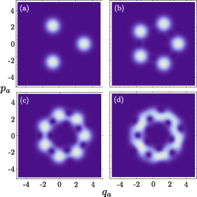
Figure 1: (Color online) Wigner function for ECSs obtained for the initial state with $\alpha=3$ and $\beta=2$ considering evolution times $t_{g}=\tau_{\mu}\frac{r}{2s}$ with $r=2$. (a) $t_{g}=\tau_{\mu}/3$ ($s=3$), (b) $t_{g}=\tau_{\mu}/5$ ($s=5$), (c) $t_{g}=\tau_{\mu}/7$ ($s=7$) and (d) $t_{g}=\tau_{\mu}/11$ ($s=11$).

We can also use our analytical solution, Eq. (16), in order to follow the dynamics at short times. In figure 2, we plot snapshots of the Wigner function considering $\alpha=3$, $\beta=0$, $r=2$ and decreasing values of $s$, i.e., increasing values of evolution time $t_{g}$, which are expressed as fractions of time scale $\tau_{\mu}=\pi/\mu$ parameter. We can see that an initial coherent state at point $\left(q_{a},p_{a}\right)=\left(3,0\right)$ starts to spread in phase (Fig.2(a) to (c)) until the “head” meets the tail of Wigner function. After that time, the state starts to interfere with itself and it is possible to resolve different packages of superposition.

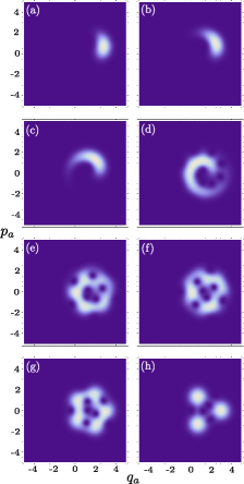
Figure 2: (Color online) Snapshots showing the evolution of the Wigner function associated with the cavity mode A for $\left|\psi_{\mathrm{field}}(0)\right\rangle=\left|3,0\right\rangle$ and $r=2$. Defining $t_{\mu}\equiv\pi/\mu$, we have: (a) $t=t_{\mu}/107$, (b) $t=t_{\mu}/61$, (c) $t=t_{\mu}/37$, (d) $t=t_{\mu}/17$, (e) $t=t_{\mu}/11$, (f) $t=t_{\mu}/7$, (g) $t=t_{\mu}/5,$ and (h) $t=t_{\mu}/3$.

IV Amplifying the nonlinear coupling

In this section, we demonstrate how to amplify the nonlinear coupling on Hamiltonian (11) by using an ensemble of $N$ identical neutral atoms. We consider all atoms with the same transition frequency $\omega_{0}+\epsilon$ between ground $\left|g\right\rangle$ and excited $\left|e\right\rangle$ states. Each atom couples with both, the classical field with Rabi frequency $\Omega$ and the polarization modes in the cavity, with frequencies $\omega_{a}$ and $\omega_{b}$. A sufficiently large interatomic separation is considered so that the dipole-dipole interactions can be neglected. In this case, we can describe the internal state of the atomic assembly by the collective pseudo-spin operators written as

$$J_{+}=\sum_{i=1}^{N}|e_{i}\rangle\langle g_{i}|,\;J_{-}=\sum_{i=1}^{N}|g_{i}\rangle\langle e_{i}|,$$

$$J_{z}=\sum_{i=1}^{N}(|e_{i}\rangle\langle e_{i}|-|g_{i}\rangle\langle g_{i}|),$$ (18)

which satisfy the angular momentum algebra. The Hamiltonian for $N$ atoms reads ($\lambda_{a}=\lambda_{b}=\lambda$)

$$H^{N} = \omega_{a}a^{\dagger}a+\omega_{b}b^{\dagger}b+\frac{\omega_{0}}{2}J_{z}+\epsilon J_{+}J_{-}$$ (19)

$$+\lambda\left[\left(a+b\right)J_{+}+\mathrm{H.c.}\right]+\Omega\left[e^{-i\omega_{0}t}J_{+}+e^{i\omega_{0}t}J_{-}\right],$$

where we consider the N atoms within a region of space whose linear dimensions are smaller than the wavelength of cavity modes. Here, the first four terms represent the free energy of the system, while the fifth describes the interaction between the collection of atoms with the cavity modes with coupling parameter given by $\lambda$. We also consider the effect of a classical driving field on the two-level atoms, described by the sixth term in Eq. (19). It is worth to note that the usual zero-point energy reference of the two level atoms was changed with the introduction of the $\epsilon$ parameter.

Following the same sequence of steps for obtaining the effective Hamiltonian (11), we first go to the interaction picture. The Hamiltonian (19) becomes

$$H_{\mathrm{int}}^{N}=H_{\mathrm{cav}}^{N}+H_{\mathrm{cef}}^{N}$$ (20)

with

$$H_{\mathrm{cav}}^{N} = \lambda[(a+b)e^{-i\Delta t}J_{+}+\textbf{H}.c.]+\epsilon J_{+}J_{-}$$

$$H_{\mathrm{cef}}^{N} = \Omega J_{+}+\Omega J_{-},$$

so that $\Delta=\Delta_{a}\equiv\omega_{a}-\omega_{0}=\Delta_{b}\equiv\omega_{b}-\omega_{0}$, i.e., the two-modes are degenerate. The first term of $H_{\mathrm{cav}}^{N}$ is the well known Dicke Hamiltonian in the interaction picture. Again, we consider that the frequencies of the cavity modes are far from resonance with the atomic transition frequency so that the dispersive condition $\left|\Delta\right|\gg\sqrt{\overline{n}_{i}}\lambda$ is satisfied. Then, using the same procedure of Ref. James (2000); James and Jerke (2007); Gamel and James (2010) we obtain the effective Hamiltonian

$$H_{\mathrm{eff}}^{N} \simeq -2\chi\left(a^{\dagger}a+b^{\dagger}b+ab^{\dagger}+a^{\dagger}b\right)J_{z}+H_{\mathrm{cef}}^{N},$$ (21)

where $\chi$ is the dispersive coupling defined previously and we are using the condition $\epsilon=2\chi$, just to remove the effective shifts in all atomic excited states. The validity of the effective Hamiltonian requires that $\Omega(\sim\sqrt{\overline{n}_{i}}\lambda)\ll\left|\Delta\right|/N$. This condition enables to disregard the influence of the classical driving field on the bimodal dispersive interaction in according with the numerical simulations from the Hamiltonian (19).

Now we go to the rotating-frame, by using the unitary transformation $U\left(t\right)=e^{-i(J_{+}+J_{-})\Omega t}$, obtaining

$$H_{\mathrm{rf}}^{N} \simeq U^{{\dagger}}H_{\mathrm{eff}}^{N}U-\dot{U}^{{\dagger}}U$$

$$= -\chi\left(a^{\dagger}a+b^{\dagger}b+ab^{\dagger}+a^{\dagger}b\right)\left(\widetilde{J}_{+}(t)+\widetilde{J}_{-}(t)\right),$$

where we have defined new collective atomic operators

$$\widetilde{J}_{+}(t) = \sum_{i=1}^{N}|+_{i}\rangle\langle-_{i}|\exp(i2\Omega t),$$

$$\widetilde{J}_{-}(t) = \sum_{i=1}^{N}|-_{i}\rangle\langle+_{i}|\exp(-i2\Omega t),$$

$$\widetilde{J}_{z} = \sum_{i=1}^{N}(|+_{i}\rangle\langle+_{i}|-|-_{i}\rangle\langle-_{i}|),$$ (23)

with $|\pm_{i}\rangle=\frac{1}{\sqrt{2}}(|e_{i}\rangle\pm|g_{i}\rangle)$. Using again the effective Hamiltonian approach, we obtain the effective interaction of many atoms with the cavity and the classical field

$$H_{\mathrm{ma}} \simeq \mu O^{2}\widetilde{J}_{z},$$ (24)

where

$$O\equiv a^{{\dagger}}a+b^{{\dagger}}b+ab^{{\dagger}}+a^{{\dagger}}b.$$ (25)

Consider that all atoms are prepared in the superposition state $\left|+_{i}\right>$ so the collective atomic state is $\prod_{i=1}^{N}\left|+_{i}\right>$. By using the eigenvalue relation

$$\tilde{J}_{z}\prod_{i=1}^{N}|+_{i}\rangle=N\prod_{i=1}^{N}|+_{i}\rangle,$$

the evolved state associated with Hamiltonian (24) is given by

$$|\Psi(t)\rangle = \exp(-i\mu O^{2}\tilde{J}_{z}t)\prod_{i=1}^{N}\left|+_{i}\right>\left|\psi_{\mathrm{field}}(0)\right>$$ (26)

$$= \exp(-iN\mu O^{2}t)\left|\psi_{\mathrm{field}}(0)\right>\prod_{i=1}^{N}\left|+_{i}\right>,$$

which means that the dynamics of the modes inside the cavity depends on the amplified quadratic beam splitter (AQBS) Hamiltonian written as

$$H_{\mathrm{AQBS}}\simeq N\mu O^{2}.$$ (27)

We can conclude that the coupling strength of the bimodal Hamiltonian can be amplified by the factor $N$, when compared with the one-atom case, Eq. (11).

In order to check the validity of this amplification, we perform a numerical calculation of linear entropy considering the exact Hamiltonian (20) considering $N=1$ to $5$. The linear entropy is a useful quantity which gives information about the purity of the system. We are interested in the linear entropy for the cavity mode described by operator $\hat{a}$ (mode A) defined as

$$\xi(t)=1-Tr_{a}\{(\rho_{a}(t))^{2}\},$$ (28)

where $\rho_{a}(t)$ is the reduced density matrix of the cavity mode A at time $t$. If $\xi=0$, the subsystem is pure and the state of the system can be written as a direct product. To perform the simulation, we consider the initial state as $\prod_{i=1}^{N}\left|+_{i}\right>\left|\psi_{\mathrm{field}}(0)\right>=\prod_{i=1}^{N}\left|+_{i}\right>\left|\alpha,\beta\right>$ with $\alpha=(q,p)=(1,0)$ and $\beta=(0,1)$. The Hamiltonian parameters are $\Delta=12.5\lambda$, $\Omega=\lambda$ and we use the value $\lambda=3\times 10^{5}$ Hz from Ref. Raimond et al. (2001). Figure 3 shows our results for linear entropy of mode A as function of time considering $N=1$ to $5$ atoms. At the initial time the linear entropy is zero, in agreement with the fact that the initial state is a direct product ($\left|\alpha\right>\otimes\left|\beta\right>\otimes\prod_{i=1}^{N}\left|+_{i}\right>$). The dynamics of linear entropy shows that the state of the atom-cavity system could not be written as a direct product except at the purification time, $t_{1}\sim\pi/\mu$. As we increase the number of atoms, the purification time decrease following the rule $t_{N}=t_{1}/N$. This is directly related with the effective coupling which goes from $\mu$ (for one atom) to $N\mu$ (for $N$ atoms).

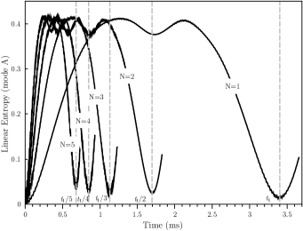
Figure 3: Linear entropy for mode A as a function of time (in microseconds) considering the evolution of initial state given by $\prod_{i=1}^{N}\left|+_{i}\right>\left|\alpha,\beta\right>$ with $\alpha=(q,p)=(1,0)$ and $\beta=(0,1)$ and different values of N. The Hamiltonian parameters are $\Delta=12.5\lambda$, $\Omega=\lambda$ with $\lambda=3\times 10^{5}$ Hz Raimond et al. (2001).

V Experimental feasibility

In this section, we discuss some aspects about current experimental feasibility of our proposal considering different experimental setups of CQED Raimond et al. (2001); Koch et al. (2011). In the experimental setup of Haroche et al. Delèglise et al. (2008); Raimond et al. (2001); Rauschenbeutel et al. (2001); Sayrin et al. (2011), Rydberg atoms (rubidium) are coupled to a microwave high quality superconductivity cavity. By considering the typical values of atom-cavity interaction being $\lambda=2\pi\times 47$ kHz for experiments with ⁸⁷Rb and setting the detuning as $\Delta=2\pi\times 235$ kHz, we estimate the value of effective frequency as $\chi=2\pi\times 9.4$ kHz. In that context, it is possible to perform a $\pi$-pulse operation using Hamiltonian (4) at the time scale given by $\tau_{\chi}\simeq\pi/\chi\simeq 0.05$ ms. Concerning the nonlinear Hamiltonian (11) the coupling parameter is given by $\mu=2\pi\times 0.94$ kHz ($\Omega\sim\lambda$), which means that the time required for a $\pi$-pulse is $\tau_{\mu}\simeq 0.5$ ms. Entangled coherent states are created at lower times: in order to create the ECS shown in Fig. 1, the time scale is given by $t_{g}=\tau_{\mu}/11\simeq 0.045$ ms to $\tau_{\mu}/3\simeq 0.17$ ms. These times are smaller than the typical Rydberg atom decay time ($\sim 30$ ms) and significatively smaller than the decoherence time associated with cavity modes ($\sim 0.13$ s) Delèglise et al. (2008); Raimond et al. (2001); Rauschenbeutel et al. (2001). In these experiments, the time of interaction between atom and cavity depends on the velocity of the atom ($100-600$ ms^-1) and varies between $100$ ns to $0.3$ ms Raimond et al. (2001). The required times for the achievement of beam-splitter Hamiltonian and the creation of ECS are both in this time range but the realization of a complete $\pi$-pulse due to the nonlinear Hamiltonian is not.

The second experimental setup, used by Rempe et al. Koch et al. (2011), consists of trapped two-level ⁸⁵Rb atoms (with atomic decay time $\sim 0.66$ $\mu$s) introduced in a small ultra-high finesse optical cavity. The atom-mode coupling is stronger than the one mentioned above being $\lambda=2\pi\times 16$ MHz. The detuning between atomic transition and the cavity can be controlled by an auxiliary laser. For $\Delta=2\pi\times 80$ MHz, we estimate the effective beam-splitter coupling as $\chi=2\pi\times 3.2$ MHz with $\tau_{\chi}\simeq 0.16$ $\mu$s and the value of nonlinear parameter is $\mu=2\pi\times 0.32$ MHz which gives $\tau_{\mu}\simeq 1.6$ $\mu$s ($\Omega\sim\lambda$). Thus, the necessary evolution times, $t_{g}$, in order to create ECS as shown in Fig. 1(b) and (d) are $0.32$ $\mu$s and $0.14$ $\mu$s, respectively. The decoherence time scale of the optical cavity used in this setup is given by $0.33$ $\mu$s, which favors both, the implementation of the $\pi$-pulse with beam-splitter interaction and the creation of ECS states but limits the implementation of $\pi$-pulses with the nonlinear Hamiltonian.

In conclusion, the comparison between both experimental setups points out that microwave cavity is a promising candidate to the implementation of the one-atom scheme. Modifications on atomic source or an auxiliar technique for slowing the atoms can be used in order to explore all the advantages of the nonlinear effective Hamiltonian. Another possibility is to use a continuous beam of atoms, as those used in Ref. Sayrin et al. (2011), so the nonlinear interaction could be stabilized for the time required by the operation. Nevertheless, although simultaneous interaction between cavity and two atoms were reported Osnaghi et al. (2011), the $N$-atoms amplification could be difficult in this particular experimental setup. Optical cavities, in contrast, are a promising system for the implementation of our propose of amplification because neutral atoms can be quasi-permanently trapped and the number of trapped atoms can be increased one-by-one Mücke et al. (2010). Another advantage is that the atom-cavity interaction is a parameter that could be easily controlled. The main problem in this setup is the decoherence of the cavity field which we expect will be solved in the near future.

VI Conclusions and perspectives

In this work, we use the effective Hamiltonian approach James (2000); James and Jerke (2007); Gamel and James (2010) in order to obtain two effective interactions between the modes of a bimodal cavity, Hamiltonians (4) and (11). By starting the system state in a product of Glauber coherent states and for specific times $t_{g}=\frac{\pi}{2\mu}\frac{r}{s}$, the nonlinear Hamiltonian drags the system to a ECS. We are able to control the number of packages manipulating either the time of evolution or effective interaction parameter between quantum and classical fields with the atomic system. Amplification of the nonlinear effective coupling between the two-modes field, described by Hamiltonian (27), can be obtained by considering a system composed of $N$ two-level atoms trapped inside a bimodal high-finesse optical cavity. We also discuss the experimental feasibility of our proposal by checking the current value of atom-cavity interaction considering both, microwave and optical cavities. We estimate the values of effective coupling strengths, $\chi$ and $\mu$, and the time scales associated with both, the application of $\pi$-pulses, $t_{\chi}$ and $t_{\mu}$, and the generation of entangled coherent states ($t_{\mathrm{ECS}}$). The $\pi$-pulse with beam-splitter Hamiltonian and the generation of ECS are possible in both scenarios. The implementation of a $\pi$-pulse with nonlinear Hamiltonian (27) requires a slightly slower atom in the microwave scheme and a longer time of decoherence in the optical setup.

Future works in this application includes the study of entanglement properties associated with the nonlinear Hamiltonian and the effects of decoherence on the entangled coherent states.

VII Acknowledgments

This work was supported by the Brazilian National Institute of Science and Technology for Quantum Information (INCT-IQ) and for Semiconductor Nanodevices (INCT-DISSE), CAPES, FAPEMIG and CNPq.

VIII Appendix: Dynamics on cavity modes

Here, we briefly explain how to obtain the evolved state associated with the QBS Hamiltonian (11). We can rewrite Eq. (12) using the unitary transformation $V=e^{\frac{\pi}{4}\left(a^{\dagger}b-ab^{\dagger}\right)}$ defining the propagator $U(t)$ as follows

$$U(t)=e^{-iH_{\mathrm{oa}}t}=Ve^{-i\mu\left(2b^{\dagger}b+1\right)^{2}t}V^{\dagger},$$ (29)

so the evolved state takes the form

$$\left|\psi_{\mathrm{field}}(t)\right\rangle=U(t)\left|\psi_{\mathrm{field}}(0)\right\rangle.$$ (30)

We are interested in the dynamics when the initial state is a direct product of coherent states

$$\left|\psi_{\mathrm{field}}(0)\right>=\left|\alpha,\beta\right>=D\left(\alpha\right)D\left(\beta\right)\left|0,0\right>,$$

where $D\left(\gamma\right)$ ($\gamma=(\alpha,\beta)$) is the displacement operator: when working with unitary transformation $V$ and the product $D\left(\alpha\right)D\left(\beta\right)$, we can use the identities:

$$V^{\dagger}D\left(\alpha\right)D\left(\beta\right)V = D\left(\frac{\alpha-\beta}{\sqrt{2}}\right)D\left(\frac{\alpha+\beta}{\sqrt{2}}\right),$$

$$VD\left(\alpha\right)D\left(\beta\right)V^{\dagger} = D\left(\frac{\beta+\alpha}{\sqrt{2}}\right)D\left(\frac{\beta-\alpha}{\sqrt{2}}\right).$$ (31)

These expressions were used in order to obtain Eq. (13). After the application of operator $V^{\dagger}$ over initial state, we obtain

$$\left|\psi_{\mathrm{field}}(t)\right\rangle = \hat{V}e^{-\frac{i}{\hbar}\mu\left(2b^{\dagger}b+1\right)^{2}t}V^{\dagger}\left|\alpha,\beta\right\rangle$$

$$= \hat{V}\left|\frac{\beta+\alpha}{\sqrt{2}}\right\rangle\otimes e^{-\frac{i}{\hbar}\mu\left(2b^{\dagger}b+1\right)^{2}t}\left|\beta_{v}\right\rangle.$$

with $\beta_{v}=\frac{\beta-\alpha}{\sqrt{2}}$. Expanding the coherent state $\left|\beta_{v}\right\rangle$ in the Fock basis on operator $\hat{n}_{b}=b^{\dagger}b$, it is straightforward to act with the second term of the propagator (29) on $\left|\beta_{v}\right\rangle$ obtaining

$$e^{-\frac{i}{\hbar}\mu\left(2b^{\dagger}b+1\right)^{2}t}\left|\beta_{v}\right\rangle = e^{-\frac{\left|\beta_{v}\right|^{2}}{2}}e^{-i\frac{\mu t}{\hbar}}\sum_{m}{\frac{\left(\beta_{v}e^{-\frac{-4i\mu t}{\hbar}}\right)^{m}}{\sqrt{m!}}}$$ (32)

$$\times e^{-\frac{4i\mu m^{2}t}{\hbar}}\left|m\right\rangle.$$

This kind of superposition of Fock state is known as generalized coherent state (GCS), which was introduced by Titulaer and Glauber Titulaer and Glauber (1966). At times given by $t_{g}=\frac{\pi}{2\mu}\frac{r}{s}$, it is possible to rewrite the GCS state given by Eq. (32) as a superposition of coherent states J. Banerji (2001)

$$e^{-\frac{i}{\hbar}\mu\left(2b^{\dagger}b+1\right)^{2}t}\left|\beta_{v}\right\rangle=\sum_{p=0}^{l-1}a_{p}^{(r,s)}\left|\beta_{p}\right\rangle$$

with $\beta_{p}=\beta_{v}e^{-2i\theta_{p}}$ and $\theta_{p}=\frac{2\mu}{\hbar}+\pi\frac{p}{l}$. Using the last result, we write the evolved state as:

$$\left|\psi_{\mathrm{field}}(t)\right\rangle=\sum_{p=0}^{l-1}a_{p}^{(r,s)}\hat{V}\left|\frac{\beta+\alpha}{\sqrt{2}}\right\rangle\left|e^{-2i\theta_{p}}\frac{\beta-\alpha}{\sqrt{2}}\right\rangle.$$

Finally, using the relations (31), we arrive to Eq. (13).

References

- Raimond et al. (2001) J. M. Raimond, M. Brune, and S. Haroche, Rev. Mod. Phys. 73, 565 (2001).
- Bertet et al. (2002) P. Bertet, A. Auffeves, P. Maioli, S. Osnaghi, T. Meunier, M. Brune, J. M. Raimond, and S. Haroche, Phys. Rev. Lett. 89, 200402 (2002).
- Delèglise et al. (2008) S. Delèglise, I. Dotsenko, C. Sayrin, M. Brune, J. M. Raimond, and S. Haroche, Nature 455, 510 (2008).
- Wigner (1932) E. Wigner, Phys. Rev. 40, 749 (1932).
- Hillery et al. (1984) M. Hillery, R. F. O’Connell, M. O. Scully, and E. P. Wigner, Phys. Rep. 106, 121 (1984).
- Koch et al. (2011) Markus Koch, Christian Sames, Maximiliam Balbach, Haytham Chibani, Alexander Kubanek, Karim Murr, Tatjana Wilk, and Gerhard Rempe, Phys. Rev. Lett. 107, 023601 (2011).
- Mücke et al. (2010) M. Mücke, E. Figueroa, J. Bochmann, C. Hahn, K. Murr, S. Ritter, C. J. Villas-Bôas, and G. Rempe, Nature 465, 755 (2010).
- Kampschulte et al. (2010) Tobias Kampschulte, Wolfgang Alt, Stephan Brakhane, Martin Eckstein, René Reimann, Artur Widera, and Dieter Meschede, Phys. Rev. Lett. 105, 153603 (2010).
- Reick et al. (2010) Sebastian Reick, Wolfgang Alt, Martin Eckstein, Tobias Kampschulte, Lingbo Kong, René Reimann, Alexander Thobe, Artur Widera, and Dieter Meschede, J. Opt. Soc. Am. B 27, A152 (2010).
- Khudaverdyan et al. (2009) M. Khudaverdyan, W. Alt, T. Kampschulte, S. Reick, A. Thobe, A. Widera, and D. Meschede, Phys. Rev. Lett. 103, 123006 (2009).
- Rauschenbeutel et al. (2001) A. Rauschenbeutel, P. Bertet, S. Osnaghi, G. Nogues, M. Brune, J. M. Raimond, and S. Haroche, Phys. Rev. A 64, 050301(R) (2001).
- Messina et al. (2003) A. Messina, S. Maniscalco, and A. Napoli, J. Mod. Optics 50, 1 (2003).
- Dong et al. (2009) Y. Dong, X. Zou, S. Zhang, S. Yang, C. Li, and G. Guo, J. Mod. Optics 56, 1230 (2009).
- Gonta et al. (2009) D. Gonta, T. Radtke, and S. Fritzsche, Phys. Rev. A 79, 062319 (2009).
- Gonta et al. (2008) D. Gonta, S. Fritzsche, and T. Radtke, Phys. Rev. A 77, 062312 (2008).
- Yurke and Stoler (1986) B. Yurke and D. Stoler, Phys. Rev. Lett. 57, 13 (1986).
- Gerry et al. (2002) C. C. Gerry, A. Benmoussa, and R. A. Campos, Phys. Rev. A 66, 13804 (2002).
- Gerry (1999) C. C. Gerry, Phys. Rev. A 59, 4095 (1999).
- Agarwal et al. (1997) G. S. Agarwal, R. R. Puri, and R. P. Singh, Phys. Rev. A 56, 2249 (1997).
- Agarwal and Banerji (1998) G. S. Agarwal and J. Banerji, Phys. Rev. A 57, 3880 (1998).
- Glancy and de Vasconcelos (2008) S. Glancy and H. de Vasconcelos, J. Opt. Soc. Am. B 25, 712 (2008).
- James (2000) D. F. V. James, Fortschr. Phys. 48, 823 (2000).
- James and Jerke (2007) D. F. V. James and J. Jerke, Can. J. Phys. 85, 625 (2007).
- Gamel and James (2010) O. Gamel and D. F. V. James, Phys. Rev. A 82, 052106 (2010).
- Yang and Zhang (2011) Rong-Can Yang and Tian-Cai Zhang, Opt. Comm. 284, 3164 (2011).
- Rong-Can et al. (2011) Yang Rong-Can, Li Gang, Li Jie and Zhang Tian-Cai, Chinese Phys. B 20, 060302 (2011).
- Feng et al. (2011) Xun-Li Feng, Chunfeng Wu, Hui Sun and C. H. Oh, Phys. Rev. Lett. 103, 200501 (2009).
- Prado et al. (2006) F. O. Prado, N. G. de Almeida, M. H. Y. Moussa, and C. J. Villas-Bôas, Phys. Rev. A 73, 043803 (2006).
- T.Werlang et al. (2008) T.Werlang, R. Guzmán, F. O. Prado, and C. J. Villas-Bôas, Phys. Rev. A 78, 033820 (2008).
- Gross et al. (2010) C. Gross, T. Zibold, E. Nicklas, J. Estève, and M. Oberthaler, Nature 464, 1165 (2010).
- Bialynicka-Birula (1968) Z. Bialynicka-Birula, Phys. Rev. 173, 1207 (1968).
- Tombesi and Mecozzi (1986) P. Tombesi and A. Mecozzi, J. Opt. Soc. Am. B 4, 1700 (1986).
- Sanders (1992) B.C. Sanders, Phys. Rev. A 45, 6811 (1992).
- van Enk (2003) S.J. van Enk, Phys. Rev. Lett. 91, 017902 (2003).
- Solano et al. (2001) E. Solano, R. L. de Matos Filho, and N. Zagury, Phys. Rev. Lett. 87, 060402 (2001).
- Zou et al. (2005) X. B. Zou, K. Pahlke, and W. Mathis, Eur. Phys. J. D 33, 297 (2005).
- Turchette et al. (1995) Q. A. Turchette, C. J. Hood, W. Lange, H. Mabuchi, and H. J. Kimble, Phys. Rev. Lett. 75, 4710 (1995).
- Duan and Kimble (2004) L.-M. Duan and H. J. Kimble, Phys. Rev. Lett. 92, 127902 (2004).
- Savage et al. (1990) C. M. Savage, S. L. Braunstein, and D. F. Walls, Opt. Lett. 15, 628 (1990).
- Kim et al. (2002) M. S. Kim, W. Son, V. Bužek, and P. L. Knight, Phys. Rev. A 65, 032323 (2002).
- Glauber (1963) R. J. Glauber, Phys. Rev. 131, 2766 (1963).
- Lutterbach and Davidovich (1997) L. G. Lutterbach and L. Davidovich, Phys. Rev. Lett. 78, 2547 (1997).
- Nogues et al. (2000) G. Nogues, A. Rauschenbeutel, S. Osnaghi, P. Bertet, M. Brune,, J. M. Raimond, S. Haroche, L. G. Lutterbach, and L. Davidovich, Phys. Rev. A 62, 54101 (2000).
- Sayrin et al. (2011) Clément Sayrin, Igor Dotsenko, Xingxing Zhou, Bruno Peaudecerf, Théo Rybarczyk, Sébastien Gleyzes, Pierre Rouchon, Mazyar Mirrahimi, Hadis Amini, Michel Brune, Jean-Michel Raimond, and Serge Haroche, Nature 477, 77 (2011).
- Osnaghi et al. (2011) S. Osnaghi, P. Bertet, A. Auffeves, P. Maioli, M. Brune, J.M. Raimond, and S. Haroche, Phys. Rev. Lett. 87, 037902 (2001).
- Titulaer and Glauber (1966) U. M. Titulaer and R. J. Glauber, Phys. Rev. 145, 1041 (1966).
- J. Banerji (2001) J. Banerji, PRAMANA- J. Phys. 56, 267 (2001).