The faint-end slope of the redshift 5.7 Ly$\alpha$ luminosity function

Abstract

Using new Keck DEIMOS spectroscopy, we examine the origin of the steep number counts of ultra-faint emission-line galaxies recently reported by Dressler et al. (2011). We confirm six Ly$\alpha$ emitters (LAEs), three of which have significant asymmetric line profiles with prominent wings extending 300-400 km s^-1 redward of the peak emission. With these six LAEs, we revise our previous estimate of the number of faint LAEs in the Dressler et al. survey. Combining these data with the density of bright LAEs in the Cosmic Origins Survey and Subaru Deep Field provides the best constraints to date on the redshift 5.7 LAE luminosity function (LF). Schechter function parameters, $\phi^{*}=4.5\times 10^{-4}$ Mpc^-3, $L^{*}=9.1\times 10^{42}$ erg s^-1, and $\alpha=-1.70$, are estimated using a maximum likelihood technique with a model for slit losses. To place this result in the context of the UV-selected galaxy population, we investigate how various parameterizations of the Ly$\alpha$ equivalent width distribution, along with the measured UV-continuum LF, affect shape and normalization of the Ly$\alpha$ LF. The nominal model, which uses $z\sim 6$ equivalent widths from the literature, falls short of the observed space density of LAEs at the bright end, possibly indicating a need for higher equivalent widths. This parameterization of the equivalent width distribution implies that as many as 50% of our faintest LAEs should have $M_{UV}>-18.0$, rendering them undetectable in even the deepest Hubble Space Telescope surveys at this redshift. Hence, ultra-deep emission-line surveys find some of the faintest galaxies ever observed at the end of the reionization epoch. Such faint galaxies likely enrich the intergalactic medium with metals and maintain its ionized state. Observations of these objects provide a glimpse of the building blocks of present-day galaxies at an early time.

1. Introduction

Observations of galaxies in the post-reionization epoch ($z\sim 4-6$) measure the growth of young objects in an early Universe. Over these redshifts, galaxies assemble into the active systems that we observe during the peak of cosmic star-formation at $z\sim 2-3$. These galaxies drive winds, which play a critical role in the metal enrichment of the intergalactic medium (IGM; Oppenheimer et al. 2009; Martin et al. 2010). Additionally, observations of galaxies in the post-reionization era provide a baseline for understanding the earliest star formation and reionization of the IGM at $z>7$.

Studies of both Lyman Break Galaxies (LBGs; Bouwens et al. 2007) and Ly$\alpha$ emitters (LAEs; Rhoads et al. 2000; Shimasaku et al. 2006; Gronwall et al. 2007; Ouchi et al. 2008, 2010; Hu et al. 2010; Kashikawa et al. 2011) in the post-reionization era provide complementary views of early star formation and galaxy evolution. The escape of Ly$\alpha$ photons from the interstellar media of galaxies is strongly influenced by galactic outflows. Typically, observable emission results when photons are redshifted out of resonance with the systemic velocity of the host galaxy (Shapley et al., 2003; Steidel et al., 2010, 2011). As a result, the comparison between LAEs and LBGs contains information about star formation driven galactic winds. For example, the space density of UV-luminous galaxies declines with increasing redshift at $z\sim 4-6$, while Ly$\alpha$– luminous galaxies maintain an approximately constant space density (Bouwens et al., 2007; Ouchi et al., 2008). The direct implication of these results is that Ly$\alpha$ photons more readily escape from galaxies at higher redshifts, possibly due to decreasing dust or the increased presence of gaseous outflows. Nevertheless, current conclusions must be drawn from limited data, as narrowband imaging observations leave the faint-end of the Ly$\alpha$ luminosity function (LF) unconstrained.

Looking to the end of reionization, it is still debated whether galaxies produced enough ionizing photons to prevent recombination in the IGM. It is often argued that galaxies fainter than those present in the deepest Hubble Space Telescope (HST) surveys are needed to produce enough ionizing photons to balance recombinations in the IGM (Yan & Windhorst, 2004; Salvaterra et al., 2011; Finlator et al., 2011). Because of this requirement for fainter objects, LAE surveys at this redshift are useful, as they can identify galaxies that cannot be detected by other means. As an example, an LAE with $L=10^{42}$ erg s^-1 and rest-frame equivalent width $W_{0}>$ 80 Å would imply a UV-luminosity of $M_{UV}>-18.0$ — a level too faint to be detected in the Hubble Ultra Deep Field (Bouwens et al., 2006). Identifying very faint LAEs can shed new light on the ionizing photon budget by including sources with continuum luminosities that have never been probed in the epoch of reionization.

In addition, studies of LAEs in the post-reionization era are crucial if we aim to determine the neutral hydrogen fraction from Ly$\alpha$ emission. Measurements of Ly$\alpha$ equivalent widths, line profiles, clustering, and the LF will all be impacted by neutral hydrogen (Miralda-Escudé et al., 2000; Furlanetto et al., 2006; Dijkstra et al., 2007a, b; McQuinn et al., 2007; Dayal et al., 2008; Schenker et al., 2011), but quantifying these effects will require robust measurements in the post-reionization era for comparison. Because galaxies in a partially neutral IGM are thought to reside in bubbles ionized by their own star-formation, luminosity dependent trends are expected (Ono et al., 2011). By measuring only bright LAEs, narrowband imaging provides an incomplete view of these star-forming galaxies.

Clearly, samples of faint LAEs are required to better understand galaxies and the IGM at $z>4$. To detect these objects, spectroscopic searches are necessary to increase the contrast with the sky background. Blind spectroscopic searches for LAEs have now successfully identified galaxies at $3<z<6$ (Santos et al. 2004; Martin et al. 2008, hereafter Paper I, Rauch et al. 2008; Sawicki et al. 2008; Cassata et al. 2011). In Dressler et al. (2011, hereafter Paper II) we presented first results from a new Multislit Narrowband Spectroscopic (MNS) survey for LAEs at $z=5.7$. In this search, we reached unprecedented depths and detected 215 LAE candidates. The faintest objects, if they are confirmed, will have luminosities that have only been seen (at this redshift) in a few lensed galaxies (Santos et al., 2004). Only 31 (14%) the LAE candidates in Paper II have fluxes bright enough to be selected through narrowband imaging ($1.0\times 10^{-17}$ erg s^-1 cm^-2).

In Paper II, we presented evidence that a high fraction of the LAE candidates are indeed LAEs, but spectroscopic confirmation is still required. In the present paper, we analyze the first results from our spectroscopic followup campaign. With a new sample of confirmed LAEs in hand, we provide the first measurement of the faint-end slope of the Ly$\alpha$ LF at redshift 5.7. We demonstrate that slit-losses can be robustly accounted for in blind-spectroscopic data by using Monte Carlo simulations within the framework of the maximum likelihood method. In fact, as we show in §6.2, this method is directly applicable to narrowband imaging data, where uncertainties often result from a non-uniform narrowband throughput.

This paper is organized as follows: in §2 we give a brief overview of the survey design. In §3 we present our spectroscopic followup observations, and in §4 we discuss the newly identified LAEs. These LAEs are used, in §5, to infer the number of LAEs that should remain in our sample, and in §6 we derive the Ly$\alpha$ LF by combining our data with those from the Subaru Deep Field (SDF) and COSMOS (Scoville et al., 2007). Prospects for improving the parameter constraints are discussed in §7. The implications of this work, including comparisons to other measurements, and a discussion of LAE properties can be found in §8. Survey completeness is described in Appendix A. Finally, in Appendix B we examine the foreground ($z\sim 0.25-1.2$) emission line galaxies and update our model for the interloper fraction that we previously presented in Paper II.

Throughout this paper we use AB magnitudes, and a $\Lambda$CDM cosmology: $H_{0}=70~{}{\rm kms^{-1}~{}Mpc^{-1}}$, $\Omega_{\Lambda}=0.7$, $\Omega_{M}=0.3$. All volumes are given in comoving units, unless otherwise stated.

2. Survey Design & Followup Strategy

The LAE candidates that we aim to confirm in this paper are selected from our spectroscopic survey, which is presented fully in Paper II. In summary, the search uses the Inamori-Magellan Areal Camera and Spectrograph (IMACS; Dressler et al. 2006) on the Magellan-Baade Telescope. To obtain blind, narrowband spectra we use a “venetian blind” slit-mask (see Figure 2 of Paper I for a schematic) and a 134 Å-wide (FWHM) blocking filter centered in the 8200Å OH-free atmospheric window. The slits on this mask cover an area of 55 arcmin², corresponding to a volume of 1.5$\times 10^{4}$ Mpc³ for Ly$\alpha$ at redshift 5.7. Emission lines that are detected are as faint as 2.5$\times 10^{-18}$ erg s^-1 cm^-2. Two fields were surveyed: one in the center of the COSMOS field (Scoville et al., 2007), and the other in the Las Campanas Infrared Survey (LCIRS) 15H field (Marzke et al., 1999). In this paper we focus on the COSMOS field, as the 15H field has only limited spectroscopic followup at this time. A more complete luminosity function, with data from both fields combined, will be the subject of a future paper.

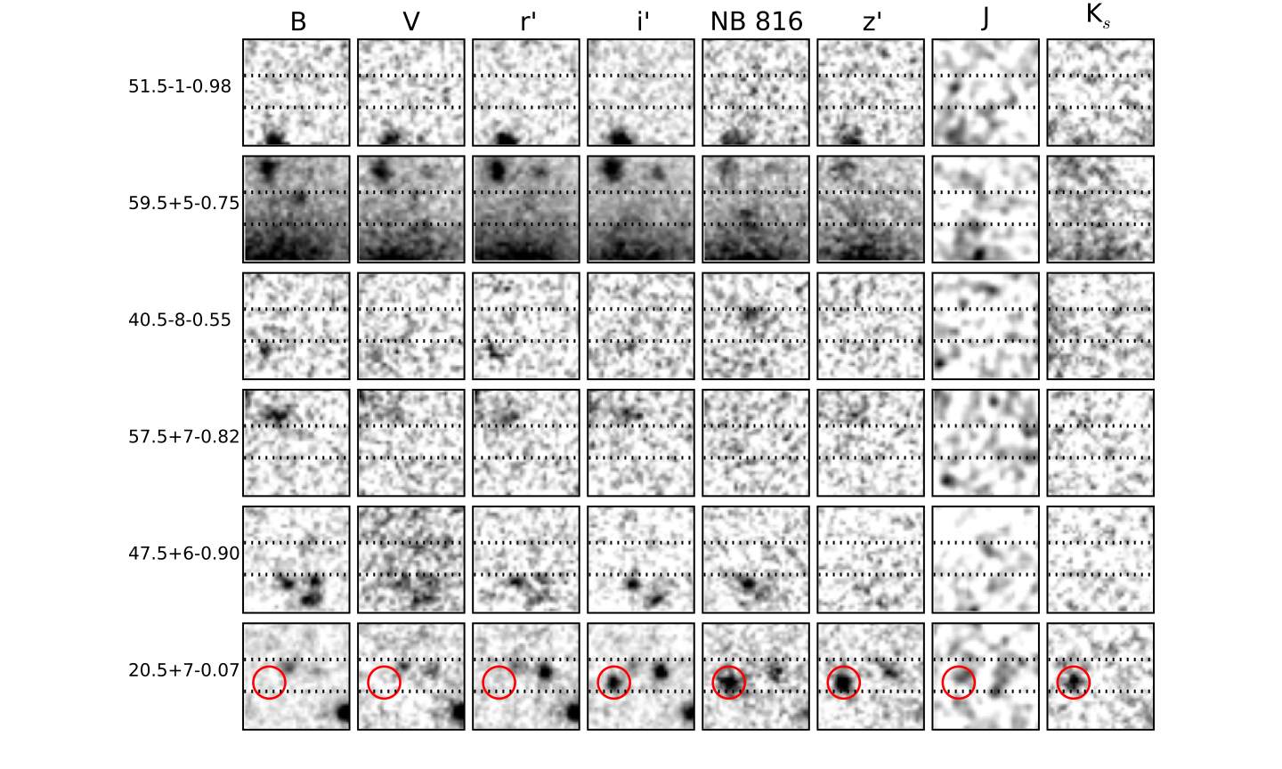
Figure 1.— Thumbnail images centered on the locations of the confirmed LAEs presented in §4. Image are 5″ on a side, and the dotted lines show the location of our slit. The Subaru (B, V, r, i, NB 816, and z), UKIRT (J), and CFHT ($K_{s}$) images are taken from the COSMOS image cutout service, hosted by the NASA/IPAC Infrared Science Archive. The $i-$ dropout near 20.5+7-0.07 (see text) is circled in red.

We identified 105 LAE candidates in the IMACS search of the COSMOS field. These objects are seen as single emission lines with no detected continuum (or, in a few cases, a possible weak continuum detection only to the red of the line). An additional 130 objects with blue continuum or multiple emission lines were identified as foreground galaxies in the search data.

Identifying the LAE candidates as genuine LAEs or foreground galaxies is not trivial. Since the positions of galaxies within the slits are not known, a large area on the sky must be searched for an optical counterpart. As a result, the normal approach of requiring an optical non-detection to distinguish foreground galaxies from LAEs is not applicable. This ambiguity is illustrated in Figure 1, which shows broadband and narrowband thumbnail images of our six confirmed LAEs (which we will discuss in §4). In most cases there are no objects falling within the slits at the spatial position of the LAEs, but in some cases there are objects nearby or outside the slits. Similarly, only 37 of the 105 LAE candidates have entries within a 2″ radius in the COSMOS photometric redshift catalog. Of these, 20 have photometric redshifts that place an emission line in our 8200Å bandpass and 17 do not.

Clearly, the faintness of our LAE candidates means that spectroscopic followup is required to determine if the detected emission line is Ly$\alpha$, or an emission line from a foreground galaxy. Under this approach, we can detect other emission lines that identify the galaxies as foreground emitters, and also observe the “smoking gun” signature of Ly$\alpha$ emission: an asymmetric line profile. In the sections below we describe our spectroscopic followup observations. The slits used to observe LAE candidates always have the same width, coordinates, and position angle (PA) as the search slits, regardless of potential optical counterparts.

3. Observations

Table 1Observation Summary

Date	Instrument	Mask Name	Mask RA	Mask Dec	Mask PA	Exposure Time	Seeing	Conditions
						(hours)	(″)
23-26 March 2009	IMACS	10hcon09	10:00:42.90	02:11:00.0	90	16.0	0.35-0.8	Clear
7 March 2010	DEIMOS	A	10:00:29.19	02:09:33.7	95	6.3	0.9-1.6	Clear
8 March 2010	DEIMOS	B	10:00:22.10	02:01:38.0	95	6.0	1.2-1.7	Cirrus
27 January 2011	DEIMOS	D	10:00:22.97	02:09:28.9	85	6.5	0.6	Clear
28 January 2011	DEIMOS	F	10:01:11.46	02:10:27.4	106	6.3	0.8	Clear

Note. — Coordinates and position angle (PA) are given for each observed mask. The slit PA, which differs from the mask PA given here, was 90 degrees for every object. Slit-widths were 1.5″.

3.1. IMACS Spectroscopic Followup

Spectroscopic followup was carried out on March 23-26 2009, using the Inamori Magellan Areal Camera (IMACS; Dressler et al. 2006) on the Magellan Baade Telescope. Conditions were clear, and the average seeing over the three nights was 0.6″. A slit width of 1.5″ was used to match the 2008 search observations, and the 200 line mm^-1 grating provided a 2 Å pixel^-1 scale to go along with the 0.2″ pixel^-1 scale of the IMACS f/2 camera. The full spectral range covered approximately 4000 - 9000 Å.

The data were reduced using the COSMOS (Carnegie Observatories System for Multi Object Spectroscopy) software package. These spectra allowed us to identify H$\alpha$, [O III], and H$\beta$ emission from galaxies. However, at this S/N and resolution neither the [O II] doublet nor the Ly$\alpha$ line profile can be resolved. Therefore, both [O II] and Ly$\alpha$ emitters appear as single emission lines in our IMACS followup spectroscopy. These single line objects are prioritized for higher-resolution spectroscopic followup with DEIMOS (see below).

3.2. DEIMOS Spectroscopic Followup

Medium resolution followup spectroscopy with DEIMOS (Faber et al., 2003) on Keck II was carried out on March 7-8, 2010 and January 27-28, 2011. Further observations scheduled March 3-4 2011 were lost entirely to poor weather. In addition to the high-priority single line emitters from our IMACS followup, the slit-masks included LAE candidates which were not targeted for IMACS followup, and those that were targeted but not recovered. (Ultimately, it was not unusual for objects that we failed to recover in IMACS followup to be robustly detected under good conditions with DEIMOS.) The observing conditions and mask positions are listed in Table 1. In the 2010 observations, poor seeing impeded our ability to recover the faintest sources and to distinguish [O II] from Ly$\alpha$ in low S/N emission line detections. Consequently, the optimal mask design in 2011 included substantial overlap with the previous year. Two LAEs identified on the March 2010 mask A (51.5-1-0.98 and 59.5+5-0.75) were also included on mask D in 2011.

Observations were made with the 830G grating, using slit-widths, position angles, and locations matched to the search data. The data were reduced using the DEEP2 DEIMOS Data Pipeline, with an updated optical model for the 830G grating (P. Capak, private communication). The January 2011 data were flux calibrated using observations of spectrophotometric standard stars, taken through a 1.5″ slit at the parallactic angle. The stars used were G191B2B, GD50, Feige 66, Feige 67, and Hz 44 (Oke, 1990; Massey & Gronwall, 1990), with reference data taken from the ESO spectrophotometric standard star database. Sensitivity functions derived from each of these stars agree to within 12%, and when Feige 66 is excluded agreement is better than 3%. In addition to the default pipeline extraction, the January 2011 spectra are extracted in 1$\farcs$8 apertures. This aperture size was chosen to match the spatial extraction in Paper II, and is appropriate given the good seeing in both the search data and January 2011 followup. No flux calibration was applied to the March 2010 data because variable seeing, at times larger than 2″, and cirrus during some of the observations, implied significant count-rate differences from frame to frame.

Line fluxes were measured from the extracted January 2011 spectra, and compared to the fluxes measured from the IMACS search data (and used in Paper II). The root mean square deviation is approximately 50%, even for bright sources. This scatter likely results from the fact that the LAE candidates are not necessarily centered in the slits, so small astrometric errors or different seeing will induce varied slit-losses from one observation to the next. In §6 we take this scatter into account when we derive the luminosity function. For consistency, all line fluxes in this paper are taken from the search data.

4. Confirmed LAEs

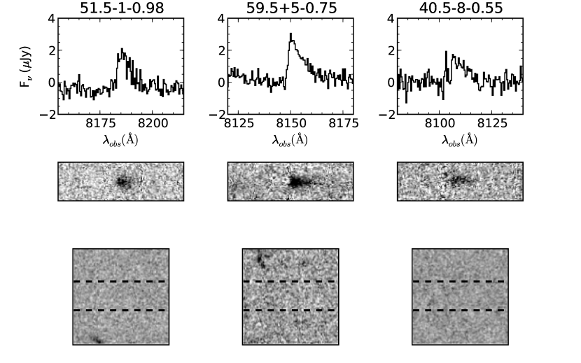
Figure 2.— Spectra of high confidence, confirmed LAEs are shown in one dimension (top row) and two dimensions (middle row; dispersion in the horizontal direction). The bottom row shows 5″  $I_{814}$ cutouts from the COSMOS ACS observations (Koekemoer et al., 2007). The detection threshold in these images depends on the sizes of galaxies, but we can estimate that undetected sources have $I_{814}$ $\gtrsim 27$ (Taniguchi et al., 2009; Henry et al., 2009). The dashed lines show the location of our 1$\farcs$5-wide slits.

Six LAEs are identified from the DEIMOS observations. Their coordinates, sizes, luminosities, velocity widths, and redshifts are listed in Table 2. In Figure 2 we show three cases of high quality Ly$\alpha$ spectra, where the asymmetric line profile makes the identification unambiguous. Little discussion is needed for these three LAEs, although we do note that the two brightest LAEs 51.5-1-0.98 and 59.5+5-0.75 are clearly spatially resolved on mask D, where they were observed under 0$\farcs$6 seeing.

When an emission line is not clearly asymmetric, more care is needed to determine if it is Ly$\alpha$. Three such cases are identified, and are shown in Figure 3 and listed in Table 2. For these galaxies, other checks are possible. First, we measure the S/N at the locations of [O III]$\lambda\lambda 4959,5007$ Å, [O II]$\lambda 3727$ Å, and H$\beta$ for the expected foreground populations. In these cases, we find that H$\beta$ and [O III] $\lambda$4959 Å are easily ruled out because other stronger emission lines would be detected. Likewise, the [O II] doublet is ruled out by the line profiles shown in Figure 3. However, we can not rule out the case where we have detected H$\alpha$ or [O III] $\lambda$5007Å, and all other lines are below the detection threshold in our DEIMOS data. While DEIMOS is efficient at 8000Å, it is about a factor of two less sensitive at blue wavelengths where we would detect [O III] from an H$\alpha$ emitter or [O II] from an [O III] emitter. Consequently, our spectra do not verify that the emission lines shown in Figure 3 are genuine LAEs.

Table 2Robust and Tentative LAEs

ID	RA	Dec	Flux	Luminosity	Mask	FWHM	Redshift	$\sigma$
	(J2000)	(J2000)	($10^{-18}$ erg s-1 cm-2)	($10^{42}$ erg s-1 )		(″)		(km s-1)
51.5–1–0.98	10:00:49.766	02:10:06.448	$9.97\pm 1.34$	3.72	A&D	1.13	5.730	$163\pm 70$
40.5–8–0.55	10:01:35.446	02:07:22.911	$5.05\pm 0.63$	1.83	F	0.94	5.666	$200\pm 35$
57.5+7–0.82	09:59:59.604	02:11:37.826	$4.07\pm 0.58$	1.51	D	0.69	5.717	$187\pm 132$
59.5+5–0.75	10:00:11.686	02:12:07.171	$10.0\pm 0.59$	3.68	A&D	0.95	5.701	$184\pm 66$
47.5+6–0.90	10:00:07.145	02:09:07.808	$5.41\pm 0.70$	2.03	D	0.59	5.749	$<140$
20.5+7–0.07	10:00:00.691	02:02:24.636	$7.16\pm 0.88$	2.67	B	1.22	5.730	$<140$

The lack of any imaged counterparts within the slits for 57.5+70.82 and 47.5+6-0.90 (Figures 1 and 3) suggests that emission lines may indeed by Ly$\alpha$. We next ask whether the implied high equivalent width would rule out H$\alpha$ or [O III] emission. For an optical counterpart to be undetected in the Subaru $i$-band and the ACS $I_{814}$  it must be fainter than about 27th magnitude (AB; Henry et al. 2009; Taniguchi et al. 2009). This gives observed-frame equivalent width limits of $W>160$ and 210 Å for these two candidates. If, on the other hand, the correct optical counterpart is one of the objects detected, but outside the slit, we would still expect a large equivalent width because the true line flux would be significantly attenuated by our slit. Nevertheless, using the COSMOS NB816 catalogs which we derived in Paper II, we find that 18-23% of H$\alpha$ and [O III] lines have equivalent widths higher than these thresholds. Since the extrapolated counts of H$\alpha$ and [O III] emitters from Paper II  are substantial, the high-equivalent width subset of these foreground populations could exist in similar numbers to the LAEs. Nevertheless, it is unlikely that both 57.5+7-0.82 and 47.5+6-0.90 are foreground interlopers.

One LAE candidate in Figure 3 has not been discussed so far: 20.5+7-0.02. Like the two other uncertain candidates, we can not rule out H$\alpha$ or [O III] from the spectrum alone. (Although, we note that this object was observed under very poor seeing in March 2010, so future observations should confirm or rule out this LAE candidate.) However, the $I_{814}$ postage stamp contains multiple objects. We explore this further by examining the multi-wavelength photometry from the COSMOS survey. Thumbnail images are shown in Figure 1; remarkably, an object 1$\farcs$3 east of our detected emission shows the appearance of an $i-$dropout (circled in Figures 1 and 3). If the detected emission is ultimately confirmed to be Ly$\alpha$, we may have observed a fainter companion galaxy. However, the bluer foreground galaxy lying near the center of the thumbnail image is more closely aligned with the detected emission, but its redshift is uncertain. Due to its faintness, this galaxy is not included in the COSMOS photometric redshift catalog.

In summary, we find three certain LAEs with clear asymmetric profiles and three plausible LAEs, where the blue sensitivity of our followup spectroscopy is insufficient to rule out all cases of H$\alpha$ and [O III] $\lambda$5007Å. In the sections that follow we derive Ly$\alpha$ LFs for two cases: the “3 LAE LF,” where only the robustly identified LAEs are included, and also the “6 LAE LF”, where both the robust and plausible LAEs are included.

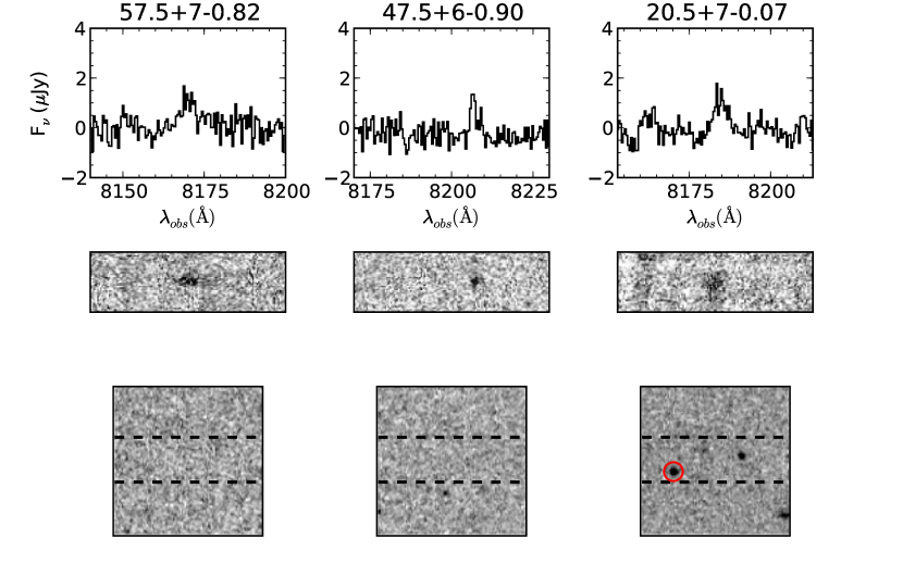
Figure 3.— Same as Figure 2, but for less certain Ly$\alpha$ identifications. The $i-$ dropout near 20.5+7-0.07 (see text) is circled in red.

5. LAE and Foreground Galaxy Identification Rates

In order to derive the Ly$\alpha$ LF, we must address the question of how many LAEs remain in our survey that have not yet been spectroscopically confirmed. To do this, we supplement our IMACS and DEIMOS spectroscopy with COSMOS photometric redshifts in order to identify as many foreground objects as possible.

To use the photometric redshifts, we must first define what we refer to as a foreground photometric match. As can be seen in Figure 1, nearby objects are present even around the robustly identified LAEs, so we can not identify foreground interlopers by the presence of optical counterparts. However, the situation is significantly improved with the COSMOS photometric redshifts (Ilbert et al., 2009), because the galaxy templates contain emission lines, and the NB816 band is included in the photometric redshift derivation. The consequence of this approach, is that– if line emission is significant in the NB816 band– the photometric redshifts become “tuned” to the precise redshifts of our foreground populations. For the NB816 filter, these redshifts are: $z=1.17-1.2$ for [O II] $\lambda$3727 Å, $z=0.62-0.69$ for [O III]$\lambda\lambda$4959, 5007 Å, and H$\beta$, and $z=0.20-0.25$ for H$\alpha$ and [S II] $\lambda\lambda$6716, 6731. To find photometric matches with all of our emission line galaxies, we search to a radius of 2″ from the slit-center. This gives 20/105 matches among the LAE candidates, and 77/130 matches among objects identified as foreground galaxies in the search data. With the caveat that this technique cannot distinguish [O III] $\lambda$5007 Å from [O III] $\lambda$4959 Å or H$\beta$, and possibly H$\alpha$ from [S II] $\lambda\lambda$6716, 6731 Å, spectroscopic followup shows that photometric matches provide the correct redshift identification in 24/24 observed cases.

In Table 3 we list the counts of foreground galaxies, LAEs, and unidentified objects by flux bins. Line fluxes are defined in the first column, and are established to correspond to 0.2 dex bins centered at log$(L/{\rm erg~{}s^{-1}})=42.1,42.3,42.5...$ for Ly$\alpha$ at redshift 5.7. The total number of emission line galaxies in the survey is given in column two, and broken into LAE candidates and foreground galaxies (both from the search data) in columns three and four. Column five lists all foreground emission lines that we have identified to date, including objects that were initially LAE candidates but have foreground photometric matches or spectroscopic identifications. Columns six and seven list the counts of confirmed LAEs for the six and three LAE cases, respectively. The final column (eight) lists the remaining unidentified LAE candidates. The sum of these unidentified object counts plus the six likely confirmed LAEs represent an absolute upper limit on the counts of faint LAEs in COSMOS. For accounting purposes, it should be noted that this conservative upper limit, plus the identified foreground galaxies column are equal to the $N_{obj}$ given in the second column. Additionally, in these binned counts we have excluded ten emitters fainter than log($F$ / erg s^-1 cm^-2) $=-17.57$ and two brighter than $-15.57$.

Table 3LAE and Foreground Counts

log $F$	$N_{obj}$	LAE candidates	Search Data Foregrounds	Identified Foregrounds	LAEs (all)	LAEs (secure)	Unidentified
-17.47	42	32	10	19	1	0	22
-17.27	54	26	28	39	2	1	13
-17.07	45	26	19	33	3	2	9
-16.87	30	9	21	24	0	0	6
-16.67	16	3	13	14	0	0	2
-16.47	14	0	14	14	0	0	0
-16.27	13	1	12	13	0	0	0
-16.07	6	0	6	6	0	0	0
-15.87	2	0	2	2	0	0	0
-15.67	1	0	1	1	0	0	0

Note. — Number counts are given for the various categories of objects in the search data, as well as after followup observations. Columns two through four are based strictly on the search data, while the remaining columns take our spectroscopic followup results into consideration. The final column gives the number counts of LAE candidates which have no spectroscopic or photometric identification.

We next aim to infer, from our spectroscopy, the number of LAEs and foreground galaxies that we expect to find among the unidentified line emitters in Table 3. For this inference, we consider only the spectroscopic identifications of objects without photometric matches, as the unidentified objects, by definition, exclude these matches. Additionally, we examine only the three faintest flux bins given in Table 3. The brighter bins contain only small numbers of LAE candidates, and none of these objects that lack photometric matches have been observed with DEIMOS. Table 4 quantifies these foreground and LAE identifications. While the numbers of galaxies with spectra remain small, no specific population of foreground emitter or LAEs appears to dominate. (Although we will discuss the significant presence of H$\beta$ emitters in Appendix B).

In order to calculate the number of LAEs that are likely present among the unidentified objects, we must recognize that these objects consist of two sub-classes. First, there are 27 galaxies where the low-resolution IMACS followup confirmed a single emission line, but was unable to resolve the [O II]  doublet. Followup spectroscopy with DEIMOS showed that these objects are predominantly [O II] and Ly$\alpha$, but, to date, not all of them have been targeted for higher-resolution spectroscopy. On the other hand, the many galaxies which have no IMACS followup are observed to be a mix of Ly$\alpha$ and all of the other bright rest-frame optical emission lines. These two sub-categories of emission line galaxies populate the number counts of unidentified emitters in Table 3, but the former has a higher LAE fraction. Therefore, we split these counts, and give LAE fractions appropriate for each sub-category in Table 4. The total numbers of inferred LAEs are calculated for both the 3 LAE LF and also the 6 LAE LF.

Table 4LAE and Foreground Rates among line emitters with no photometric matches

log $F$	$N_{spec}$	No ID	Ly$\alpha$ (all)	Ly$\alpha$ (secure)	H$\alpha$	H$\beta$	[O III]	[O II]	Other	Inferred LAEs (all)	Inferred LAEs (secure)
Line Emitters with no IMACS followup
-17.47	8	19	1	0	1	2	1	2	1	2.1	0
-17.27	7	9	2	1	0	3	0	1	1	2.3	1.1
-17.07	6	6	3	2	1	0	0	3	1	1.8	1.2
IMACS confirmed single line emitters
-17.47	2	3	0	0	0	0	0	2	0	0	0
-17.27	2	4	1	1	0	1	0	0	0	2	2
-17.17	3	3	2	1	0	0	0	1	0	2	1
Total LAEs (Confirmed and Inferred)
-17.47										3.1	0
-17.27										6.3	4.1
-17.17										6.8	4.2

6. The Ly$\alpha$ luminosity function

6.1. Direct Calculation

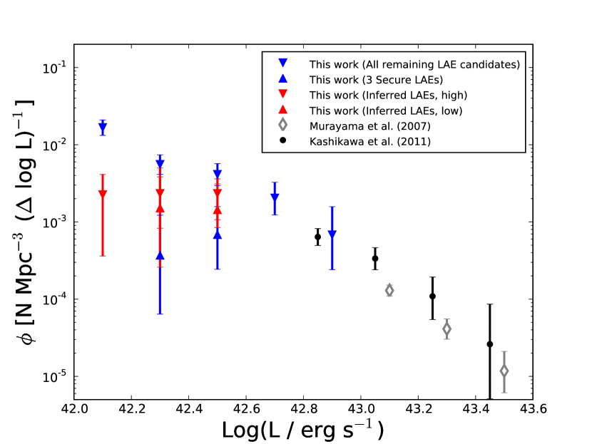
Figure 4.— The discrete luminosity functions derived from our blind spectroscopic sample are shown in red (inferred from the low, 3 LAE and high or 6 LAE samples). The more conservative limits are shown in blue. For comparison, the bright-end data from the Subaru Deep Field (SDF;Shimasaku et al. 2006; Kashikawa et al. 2011) and COSMOS (Murayama et al., 2007) are shown. The SDF data shown here exclude the faintest candidates reported by Kashikawa et al. (2011), where the spectroscopic confirmation rate is low.

With the counts of LAEs given in Tables 3 and 4, a direct derivation of the LF is straightforward. The volume subtended by the slits in our search mask is 1.5$\times 10^{4}$ Mpc³. Correcting these counts for the detection completeness (Appendix A), we derive the conservative lower and upper limits (blue triangles). Under this approach, the lower limit is derived by including only the three robustly identified objects. The conservative upper limit, on the other hand, also includes the three tentatively identified LAEs and all of the unidentified objects in Table 3. These discrete LFs are plotted in Figure 4. No slit-loss corrections are applied at this stage; they will be addressed §6.2.

In order to derive a meaningful constraint on the faint-end slope of the LF, data that cover the bright-end and the knee are needed. For this calculation, we draw on LAE catalogs available in COSMOS (Murayama et al., 2007) and the Subaru Deep Field (SDF; Kashikawa et al. 2011, K. Shimasaku, private communication). While spectroscopic observations are more sensitive to low equivalent width emission, no systematic correction is needed, because the contribution from these sources is negligible. No LAE candidates are seen with (convincingly) detected continuum in the IMACS search data, implying rest-frame equivalent widths, $W_{0}\gtrsim 7-10$ Å. Therefore, the combination of these two different survey methods is valid.

The COSMOS (Murayama et al., 2007), and SDF (Kashikawa et al. 2011) samples are derived in similar ways. Both are selected from Subaru/SuprimeCam observations through the NB816 filter. However, the color cuts used to select the LAEs are not the same: Murayama et al. require $iz-NB816>0.7$, while the SDF LAEs are selected with $i-NB816>1.5$. Comparison of these catalogs shows only a small difference. All of the galaxies in the SDF catalog have $iz-NB816>0.67$, and only two have $iz-NB816<$ 0.70. Conversely, 83% of the Murayama et al. (COSMOS) catalog meets the SDF color cut. Since the suitability of one color cut over another is unknown, we make no corrections, but note that this level of systematic uncertainty is present in the data.

For the SDF sample, we calculate the line fluxes and Ly$\alpha$ luminosities, taking into account the non-uniform transmission of the NB816 filter (see Figure 5). These quantities are calculated from the 2″ aperture $z-$band and NB816 magnitudes, following the prescription in Kashikawa et al. (2011). When redshifts are unknown, they are fixed to $z=5.70$ so that the line is assumed to fall at the center of the filter bandpass. A single aperture correction is applied to all galaxies in this sample, which we estimate by comparing SExtractor (Bertin & Arnouts, 1996) MAG_AUTO magnitudes to the 2″ diameter magnitudes. This approach is preferable to simply adopting the MAG_AUTO magnitudes, which are unreliable at low S/N. From this comparison, we find a median aperture correction of -0.38 magnitudes to the NB816 photometry, indicating a +0.15 dex correction to the Ly$\alpha$ luminosity.

Considerable efforts to follow up the SDF sample have confirmed 46/89 LAE candidates and identified four [O II] emitters (Shimasaku et al., 2006; Kashikawa et al., 2011). The spectroscopic confirmation is highly complete at the bright end, but falls off to fainter luminosities. Excluding the [O II] emitters, and dividing the sample at $L(2\arcsec)=10^{42.6}$ erg s^-1, 31/36 (86%) of the brighter LAE candidates are confirmed, but only 15/39 (38%) of the fainter candidates are confirmed. Since narrowband imaging is subject to the selection of spurious (no emission line) sources at faint magnitudes, we restrict the sample to $L(2\arcsec)>10^{42.6}$ erg s^-1 where the confirmation rate is high. The five unconfirmed LAE candidates with these bright luminosities are included, as their unconfirmed status is likely the result of slit-mask design.

We calculate the differential luminosity function for the SDF LAEs by determining the effective volume over which each object can be both detected with NB816 (2″) $<26$, and selected with $i-NB816>1.5$. Within the 725 arcmin² of the SDF, these volumes range from $1.7\times 10^{5}$ Mpc³ for $L\sim 10^{42.6}$ erg s^-1 to 2.3 $\times 10^{5}$ Mpc³ for $L>10^{43}$ erg s^-1. For the five LAEs that are not spectroscopically confirmed we adopt an effective volume defined by the redshift range that corresponds to the FWHM of the NB816 filter: 1.9 $\times 10^{5}$ Mpc³. Next, a completeness correction for each object, as a function of its NB816 magnitude (K. Shimasaku, private communication), is applied. The differential luminosity function from the SDF is plotted in Figure 4.

Figure 5.— The NB816 throughput (dashed line) is non-uniform, so the emission line flux inferred from NB816 magnitudes will, on average, be underestimated. For comparison, we show the much squarer transmission profile of the filter used in this work (solid line).

Combined with the SDF, COSMOS is an excellent complement, covering nearly 10 times the area to a shallower depth. Over 1.86 degrees², Murayama et al. (2007) report 111 LAEs. Spectroscopic redshifts for this sample are unavailable, so like the unconfirmed SDF LAEs, we adopt a volume spanned by the FWHM of the filter bandpass: $1.9\times 10^{6}$ Mpc³. Likewise, line fluxes and luminosities are calculated in the same way that was done for the SDF LAEs. However, we note that, for the COSMOS sample, the best estimate of the total luminosities are taken from 3″ diameter apertures. In Figure 4 we show the differential luminosity function for the 65 LAEs brighter than 10⁴³ erg s^-1. Although the precise completeness of this sample is not known, comparison to the SDF LF shows that the COSMOS LAE catalog is complete above this conservative cut. As we will show below, the slightly lower normalization of the COSMOS Ly$\alpha$ LF is actually a shift in luminosity of about 0.05 dex, which results from the assumption that all of these emission lines are centered in the NB816 bandpass.

6.2. Maximum Likelihood Derivation

So far, in our calculation of the Ly$\alpha$ LF shown in Figure 4, we have assumed that the observed luminosity, $L$, is a good approximation to the true luminosity $L_{0}$. However, in some cases, this approximation will fail. In the blind spectroscopic data, a luminous galaxy can be detected as a faint object if it falls outside of the slit. Similarly, with narrowband imaging through the non-uniform transmission of the NB816 filter, luminous galaxies can be observed with faint luminosities if the line is transmitted far from the center of the bandpass. Not only are the luminosities altered by slit and filter transmission effects, but the volume from which a galaxy is drawn also becomes uncertain. Relative to fainter galaxies, intrinsically bright line emission can be detected over a larger volume because these galaxies can be observed further from the slit- or bandpass- center. In short, blind-spectroscopic observations and narrowband imaging surveys are subject to the same problems: when precise slit-positions or redshifts are unknown, true luminosities are uncertain and volumes are not well-defined.

A maximum likelihood approach to the luminosity function parameter estimation (e. g. Sandage, Tammann, & Yahil 1979; STY) offers a natural solution to this problem, as it allows the flexibility to model these effects of uncertain luminosity and volume. With a Monte Carlo simulation (described below) we can determine the probability $k(L_{0}\rightarrow L)$ that a galaxy with some true luminosity, $L_{0}$, will be observed with some other luminosity $L$ (Gronwall et al., 2007; Reddy et al., 2008). The luminosity function that we observe as a function of $L$ is then a convolution of the true luminosity function with these kernels, $k(L_{0}\rightarrow L)$:

$$\phi(L)=\int k(L_{0}\rightarrow L)\phi(L_{0})dL_{0}.$$ (1)

Here, $\phi(L_{0})$ represents the Schechter parameterization of the luminosity function: $\phi(x)dx=\phi^{*}x^{\alpha}e^{-x}dx$ , where $x=L/L^{*}$. In the limit where there is no scatter between $L_{0}$ and $L$, $k(L_{0}\rightarrow L)$ becomes a delta function, and Equation 1 reduces to $\phi(L)=\phi(L_{0})$.

This treatment can be applied directly to the STY maximum likelihood parameter estimation, where we choose $\alpha$ and $L^{*}$ that maximize the likelihood of observing the set of $N$ galaxies in our sample, with luminosities $L_{i}$:

$$\mathcal{L}(\alpha,L^{*})=\prod_{i=1}^{N}\frac{\phi(L_{i})}{\int\phi(L)dL}.$$ (2)

Including the convolution shown in Equation 1, the likelihood function becomes:

$$\mathcal{L}(\alpha,L^{*})=\prod_{i=1}^{n}\frac{\int k(L_{0}\rightarrow L_{i})\phi(L_{0})dL_{0}}{\int dL\int dL_{0}k(L_{0}\rightarrow L)\phi(L_{0})}$$ (3)

Since $\phi^{*}$ appears in the numerator and denominator, the normalization is set by the number of galaxies that are observed. To calculate the normalization, while accounting for the covariance between $\alpha$, $\phi^{*}$, and $L^{*}$, we calculate the number of galaxies, $N^{\prime}$, predicted by each model:

$$N^{\prime}=\int dL\int dL_{0}k(L_{0}\rightarrow L)\phi(L_{0})\times Volume.$$ (4)

The appropriate survey volume here is the one that is matched to the simulation used to derive $k(L_{0}\rightarrow L)$. In the following calculations, the survey volume is not a function of luminosity, because galaxies are uniformly simulated out to some maximum distance from slit-center (or wavelength from away from the bandpass-center). Under this approach, $k(L_{0}\rightarrow L)$ reflects the incompleteness to fainter galaxies when their simulated positions/wavelengths render them undetectable. Finally, we include the (Poisson) probability of observing the $N$ galaxies in our survey, given the model prediction of $N^{\prime}$:

$$\mathcal{L}(\alpha,L^{*},\phi^{*})=\mathcal{L}(\alpha,L^{*})*P(N|N^{\prime}).$$ (5)

The joint constraint from the three different surveys that we use in this paper is simply the product of the likelihood functions, $\mathcal{L}(\alpha,L^{*},\phi^{*})$, for each.

6.3. Implementation of the maximum likelihood parameter estimation

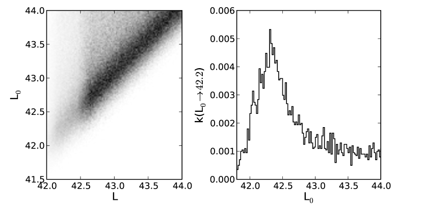
Figure 6.— Left– The convolution kernels $k(L_{0}\rightarrow L)$ describe the probability of a galaxy with luminosity $L_{0}$ being observed with some other luminosity $L$. While these probabilities are strongly peaked on the diagonal, where $L_{0}\sim L$, there is a non-trivial tail where galaxies with large $L_{0}$ are detected with faint $L$. These are galaxies that fall partially outside of slits. This example is for the 6 LAE case, so the redshift identification incompleteness is apparent at $L\lesssim 10^{42.5}$ erg s^-1. Right– A vertical slice of the left panel, taken for $L=10^{42.2}$ erg s^-1 shows the fraction of galaxies that are detected with this luminosity but in actuality have other luminosities, $L_{0}$. Again, the tail to high $L_{0}$ comes from sources that fall partially outside the slit.

Having outlined the steps needed to derive the best-fitting Schechter parameters, we next implement this method for both our spectroscopic data and bright-end data taken from the COSMOS and the SDF narrowband imaging surveys. For each of these three surveys we use Monte Carlo simulations to calculate the convolution kernels $k(L_{0}\rightarrow L)$. With these quantities in hand, we find the $\alpha$, $L^{*}$ and $\phi^{*}$ that maximize Equation 5.

6.3.1 Blind Spectroscopic Data

The quantities that determine $k(L_{0}\rightarrow L)$ for blind spectroscopy are: (1) the photometric scatter, and (2) the observed sizes of the Ly$\alpha$ emission in our 0$\farcs$5 seeing search data. As mentioned in §1, our DEIMOS observations, when compared to the IMACS search data, indicate a photometric scatter with an RMS of 40-50%, regardless of line flux. The sizes of LAEs, on the other hand, require a more careful consideration. Continuum observations show that the majority of LBGs, including those with Ly$\alpha$ emission, have compact sizes at $z\sim 6$ (Bouwens et al., 2004; Ferguson et al., 2004; Henry et al., 2010; Malhotra et al., 2011; Gronwall et al., 2011). Additionally, Hubble Space Telescope imaging of Ly$\alpha$ emission from redshift 3-4 LAEs supports the scenario where Ly$\alpha$ emission is similarly compact (Bond et al., 2010; Finkelstein et al., 2011). However, two of the securely identified LAEs are clearly resolved in the DEIMOS followup observations, so we consider the impact of size.

Because our sample is too small at this time to adopt an empirically motivated size distribution, we consider three cases to illustrate the effect of LAE sizes. We assume constant sizes of 0$\farcs$5, 0$\farcs$75, and 1$\farcs$0 (observed FWHM), and derive LAE parameter constraints (by the method described below). This test shows that, when larger sizes are adopted, the most likely values of $\phi^{*}$, $L^{*}$, and $\alpha$ are unchanged within the precision of our parameter search ($\Delta$log($L^{*}$) = 0.01, $\Delta$log($\phi^{*}$) = 0.01, and $\Delta\alpha$ = 0.05). Only the likelihood contours are slightly altered when larger sizes are used. Relative to the constraints obtained when 0.5″ FWHM are adopted, 1″ sizes result in an extension of the likelihood contours to values brighter by 0.1 dex for log($L^{*}$), and steeper by 0.1 for $\alpha$ (68% confidence). For quantifying the uncertainties, we adopt the intermediate case where all LAEs have observed FWHM = $0.75$″ in the IMACS search data.

With these assumptions, we determine $k(L_{0}\rightarrow L)$ by a Monte Carlo simulation where LAEs are randomly placed inside and near the slits, and noise is added. We consider an intrinsic luminosity range of $L_{0}=10^{41.5}-10^{44}$ erg s^-1. The lowest simulated luminosity is fainter than the limit of our search, so this allows for photometric scatter into our selection. The high-luminosity cutoff is arbitrary, but is justified since the volume density of LAEs becomes vanishingly small at this luminosity (Murayama et al., 2007). This high$-L$ cutoff determines the maximum distance from slit-center where LAEs are placed. A galaxy with $L_{0}=10^{44}$ erg s^-1 and a size of 0.75″ (FWHM) can present detectable line flux even from a distance of 1.7″ from the slit-center. Therefore, for the blind spectroscopy, the volume used in Equation 4 is 3.4$\times 10^{4}$ Mpc³.

Since $k(L_{0}\rightarrow L)$ describes the probability of a galaxy with luminosity $L_{0}$ being observed in our survey, it is appropriate to include survey completeness in the Monte Carlo simulation. This takes two forms. First, the detection incompleteness, which is derived in Appendix A, is included. Additionally, since we are deriving LFs from inferred counts, we include a redshift identification incompleteness defined as the ratio of the confirmed LAEs (columns four and five) to the inferred LAEs (columns eleven and twelve) in Table 4. The bin with zero inferred LAEs is assigned a spectroscopic completeness of zero.

Figure 6 shows $k(L_{0}\rightarrow L)$ with the spectroscopic incompleteness included for the six-LAE case. The left panel shows that, in this two dimensional space, the probability is peaked on the diagonal because the most likely true luminosity, $L_{0}$, is the one that we observe, $L$. However, a tail of galaxies with high $L_{0}$ and low observed $L$ are also present when galaxies fall partly outside of a slit. On the left-hand side of this two dimensional space, at $L<10^{42.5}$ erg s^-1, the spectroscopic incompleteness is apparent. The right panel of Figure 6 shows a vertical slice of the left panel to illustrate the fraction of galaxies at each $L_{0}$ that are detected with $L=10^{42.2}$ erg s^-1. Because of photometric scatter, there is a significant probability of a galaxy having a fainter true luminosity, $L_{0}$, than is observed. It is worth noting that, if a set of Schechter parameters are assumed, we can use this slice in Equation 1 to get $\phi(L=10^{42.2}~{}{\rm erg~{}s^{-1}})$.

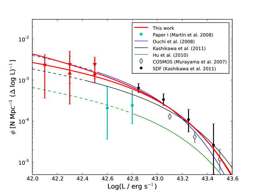
Figure 7.— Best-fit LFs to the inferred LAE counts (high and low), shown in red, are compared to other derivations of the redshift 5.7 luminosity function. Curves are dashed at luminosities where they are extrapolated beyond the data in their various studies. For the Ouchi et al. (2008); Kashikawa et al. (2011) and Hu et al. (2010) studies we show the fits for $\alpha\equiv-1.5$, which is intermediate to the values favored by our data.

6.3.2 Bright-end Narrowband Imaging Data

To calculate $k(L_{0}\rightarrow L)$ for the narrowband imaging samples, we must take two scenarios into consideration: when the redshifts of the emission lines are known, as they are for most (but not all) of the SDF LAEs, and when the redshifts are unknown, as is the case for the COSMOS narrowband imaging sample. When redshifts are unknown, emission lines with some $L_{0}$ are placed randomly at wavelengths between 8050 Å and 8250 Å. Therefore, the appropriate volumes used in Equation 4 are $3.2\times 10^{5}$ Mpc³ for the SDF and $3.0\times 10^{6}$ Mpc³ for COSMOS. Additionally, a normally distributed flux error is added, with $\sigma=2~{}{\rm or}~{}5\times 10^{-18}$ erg s^-1 cm^-2  for the SDF and COSMOS simulations.

As with the blind spectroscopic data, these Monte Carlo simulations include detection completeness. While the COSMOS narrowband imaging sample is assumed to be complete at $L>10^{43}$ erg s^-1, the SDF data must be corrected. Although the incompleteness for this sample is a function of the NB816 magnitude, it varies slowly from 75 - 90% over the range that we are interested. Furthermore, the line luminosity forms a fairly tight correlation with the NB816 magnitude, with an RMS scatter of 0.1 dex. Therefore, at each luminosity we adopt a completeness appropriate for the mean NB816 magnitude of galaxies with that luminosity.

When the redshifts of the emission lines are known, a different set of kernels is used in Equation 3. In this case, the simulation differs from the case of unknown redshifts, because the observed $L$ have been corrected for the transmission through the filter curve shown in Figure 5. Therefore, in this simulation there is no scatter between $L_{0}$ and $L$ from the unknown filter throughput. In the absence of noise, these kernels would be a set of $\delta$-functions. However, as with the case of unknown redshifts, noise and detection incompleteness are included. For the purposes of determining the normalization, we adopt the scenario used for unknown redshifts in Equation 4 for all SDF LAEs.

6.4. Results: Luminosity Function Constraints

With the various $k(L_{0}\rightarrow L)$ in hand, we evaluate Equation 5 for each survey, over a grid of $\alpha$, $L^{*}$, and $\phi^{*}$. The final likelihood function is given by the product of the individual likelihood functions, $\mathcal{L}(\alpha,L^{*},\phi^{*})$, for each survey. The parameters that maximize this quantity are given in Table 5, for both the 3-LAE and 6-LAE LFs.

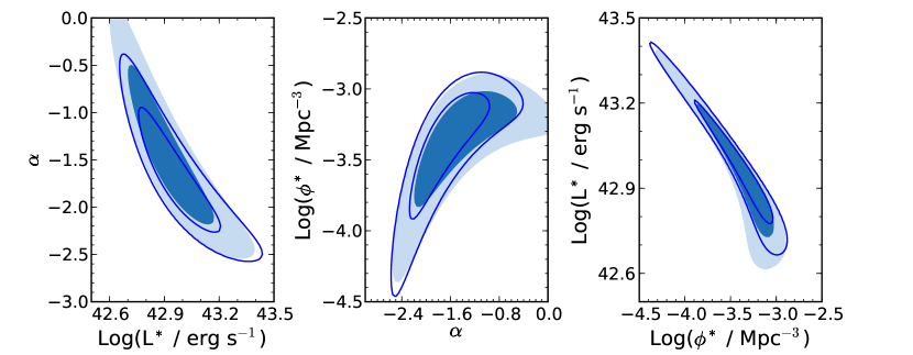
Figure 8.— Likelihood contours show the Schechter parameter constraints from the Multislit Narrowband Spectroscopic sample (this paper), combined with the bright-end narrowband imaging data from COSMOS and the SDF. The 68 and 95% confidence intervals are represented by the shaded contours for the 3 LAE LF and by the open curves for the 6 LAE LF.

Table 5Most Likely Schechter Function Parameters

Sample	log($\phi^{*}/{\rm Mpc}^{-3}$)	log($L^{*}/{\rm ergs}^{-1}$)	$\alpha$
3 LAE	$-3.29^{+0.27}_{-0.52}$	$42.91^{+0.19}_{-0.21}$	$-1.45^{+0.92}_{-0.70}$
6 LAE	$-3.35^{+0.31}_{-0.56}$	$42.96^{+0.24}_{-0.16}$	$-1.70^{+0.73}_{-0.57}$

The best-fitting Schechter-functions are plotted in Figure 7. One feature of maximum likelihood parameter estimation is that the most likely model does not always run through the data points. This is indeed the case in Figure 7. The discrete points describing the COSMOS LAEs are derived by assuming that all objects are observed through the peak of the NB816 throughput curve. Consequently, on average, the true luminosities, $L_{0}$, of these LAEs will be brighter than what we have observed. Since we model these effects with our maximum likelihood estimation, we expect the Schechter functions plotted in Figure 7 to fall above the discrete data points for the COSMOS narrowband imaging data. On the other hand, since we have taken the bandpass into account for the 85% of the SDF LAEs that are spectroscopically confirmed, we expect the most likely Schechter function to closely follow the discrete SDF points in Figure 7. In fact, if we exclude the SDF data from our fit, the bright-end of the best-fit Schechter function falls close to the same location, approximately 0.05 dex brighter than the COSMOS narrowband imaging points shown in Figures 4 and 7. Correcting these points in Figures 4 and 7 for this average attenuation, would bring them in line with the SDF data and the Schechter function fit.

Figure 8 shows the 68% and 95% confidence intervals for these parameter constraints. Clearly, owing to our small sample of faint LAEs, a large range of acceptable faint-end slopes can describe our data. However, as our spectroscopic followup becomes more complete, the luminosity function parameters will be more tightly constrained.

7. Improving the faint-end slope constraint with more followup spectroscopy

It is not surprising that the luminosity function parameter constraints which we show in Figure 8 allow a wide range of Schechter parameters. At this time the faint-end of our LF is based on only a few confirmed LAEs. Our continued efforts at followup spectroscopy will narrow the allowed parameter space by increasing the sample size. Furthermore, the addition of our 15H field, when spectroscopy is complete, will approximately double the number of LAEs over what is present in the COSMOS field.

It is therefore of interest to address how strict the constraints from our survey may ultimately prove. To explore this, we create a mock catalog of galaxies with $\phi^{*}=10^{-3.35}~{}{\rm Mpc}^{-3}$, $L^{*}=10^{42.96}~{}{\rm erg~{}s}^{-1}$, and $\alpha=-1.70$ (our 6 LAE LF in Table 5 and the contour curves in Figure 8). These galaxies are distributed throughout the volume of both our COSMOS and 15H IMACS fields, out to 1.7″ from slit-center, similar to the Monte-Carlo simulations in §6.2. Slit-losses, noise, and detection completeness are included. Finally, we assume a spectroscopic completeness of 90% at all luminosities, since achieving 100% completeness is usually impractical. The resulting sample of LAEs in both fields is approximately 40 galaxies. After regenerating the convolution kernels to include the appropriate spectroscopic completeness, we calculate the likelihood function, $\mathcal{L}(\alpha,L^{*},\phi^{*})$ over the grid of $\alpha,L^{*},\phi^{*}$ (leaving the bright-end data unchanged). Contours shown in Figure 9 illustrate the improvements in the constraints that we can expect to find from completing our spectroscopic followup. For the increased sample size in this simulation, the 68% confidence interval on the faint-end slope is reduced by 50%. Likewise, under our current constraints, the space density of LAEs at $L=10^{42}$ erg s^-1 spans a factor of 10 (68% confidence), but should be decreased to less than a factor of three when both fields are 90% complete.

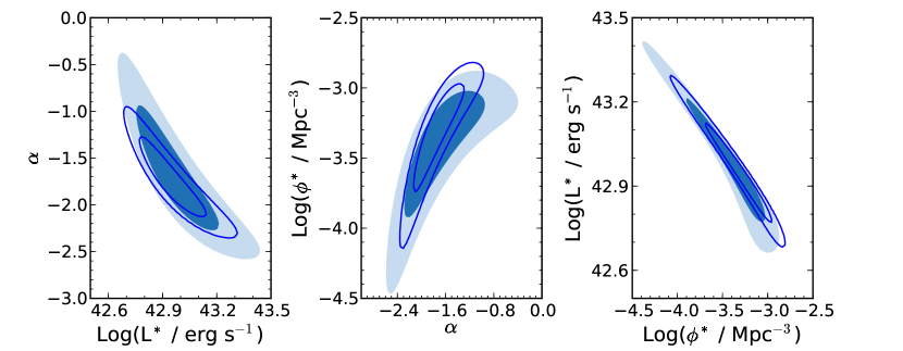
Figure 9.— Likelihood contours show the Schechter parameter constraints that we can achieve when the spectroscopic followup is 90% complete in both of our survey fields (curves). An improvement relative to our current constraints (shaded) is expected. For simplicity, we compare only the LF derived from 6 LAEs to a simulated sample derived from the 6 LAE LF Schechter parameters. The bright end data are unchanged from what we have used in this study. Contours are shown for 68 and 95% confidence.

8. Discussion

8.1. Comparison to previous measurements of the redshift 5.7 Ly$\alpha$ LF

In Figure 7 we compare the LFs derived in this work to those presented in previous studies at redshift 5.7. A number of items are readily evident. First, the shape ($\phi^{*}$ and $L^{*}$) of the LF that we derive from the SDF data is different from the shape obtained by Kashikawa et al. (2011), from the same bright-end data. This variation is not surprising, given our different analysis. Most notably, we have adopted luminosities calculated from the NB816 and $z$-band magnitudes, whereas Kashikawa et al. use luminosities derived from their followup spectroscopy. Given the uncertainties associated with estimating slit-losses, imaging-based measurements may be a better approximation to the total Ly$\alpha$ luminosity– provided that aperture magnitudes are corrected to total magnitudes, and the redshifts are used to calculate the true luminosity observed through the NB816 filter.

Figure 7 also compares our bright-end LF derivation with the similar redshift 5.7 Ly$\alpha$ LF from the Subaru/XMM-Newton Deep Survey (SXDS; Ouchi et al. 2008). While the agreement between the plotted Schechter functions is good, this may be fortuitous. Limited spectroscopic followup in the SXDS could allow significant contamination, since narrowband imaging can sometimes select LAE candidates which have no line emission at all. This point is illustrated clearly in the color magnitude plots used to select LAE candidates (Figure 7 in Ouchi et al. 2008; Figure 1 in Murayama et al. 2007; Figure 7 in Shimasaku et al. 2006). When the limit of the NB816 photometry is approached, there is significant scatter about the threshold that defines an emission line source. While the use of optical “veto” bands will eliminate some spurious emission line candidates, even this method could break down for faint galaxies, where modestly red galaxy SEDs may be undetected at bluer wavelengths. This contamination may account for the LAEs which Kashikawa et al. (2011) do not detect in followup spectroscopy. Likewise, the faintest confirmed LAEs in the SXDS (Ouchi et al., 2008) are about one magnitude brighter in NB816 than the limit of that sample. More spectroscopic followup will be needed to determine the reliability of the fainter Ly$\alpha$ candidates selected from narrowband imaging. Such observations would provide better constraints on the space density of LAEs at luminosities around the knee of the LF, and reduce the covariances shown in Figures 8 and 9.

Two other measurements deviate from the LF that we derive here: Hu et al. (2010), and Paper I. These bright and intermediate luminosity data would require a discontinuity from our new faint-end results. A Schechter function can not be fit which simultaneously goes through these data and our new data. Therefore, it is clear that both the Paper I and Hu et al. samples are incomplete. Indeed, incompleteness in the Hu et al. result is discussed in Kashikawa et al. (2011). Because Hu et al. require spectroscopic confirmation, but use shorter observations than Kashikawa et al., it is argued that the incompleteness is simply a failure to re-detect some real LAEs. On the other hand, for our pilot survey, comparison of our current completeness to the detection completeness derived in Paper I suggests that the prior estimate was overly optimistic. For the current data, near 100% completeness is reached for detections of better than 10$\sigma$ significance. Shifting the completeness curve for the present data (Appendix A) by a factor of four to five in flux allows us to revise the completeness estimate used for the shallower data in Paper I. This exercise suggests that our previous LF was 30-70% complete, rather than near 100%, as was assumed. Revising these completeness corrections would bring the Paper I points more closely in line with our new LF and the Ouchi et al. (2008) result.

In Paper II, our analysis of the foreground populations suggested that the remaining counts of LAEs followed a similar faint-end slope, with $\alpha\sim-2$. With our followup spectroscopy, we now find that the most likely slope is slightly shallower, although $\alpha=-2$ is well within the 1$\sigma$ measurement uncertainty. Nevertheless, we identify the source of this difference (for the COSMOS field) in Appendix B. Briefly, the foreground emission line galaxies that we have identified so far in our followup add up to the counts predicted by the foreground model adopted in Paper II. Since we expect that a significant fraction of the unidentified emission lines listed in Table 3 are also foreground objects, we expect these counts to be higher than the most likely model adopted in Paper II. Because of this, the fraction of LAEs among our detected emission lines will be smaller than we previously estimated in Paper II. As we show in Appendix B, the most likely cause of this underestimation is a strong presence of H$\beta$ emitters from an overdensity at $z\sim 0.68$ in the COSMOS field.

Finally, we note that the cosmic variance for our faint LAE sample, at this time, makes a negligible contribution to the error budget because the Poisson errors on our small sample are much larger than the cosmic variance. On the other hand, at the bright end, the excellent agreement between the narrowband imaging samples from COSMOS, the SDF, and the SXDS is better than the approximately 20-30% cosmic variance that we expect for these surveys (Trenti & Stiavelli, 2009).

8.2. Comparison to faint Ly$\alpha$ LFs at lower redshift

So far, we have compared our Ly$\alpha$ LF to previously measured Ly$\alpha$ LFs at redshift 5.7. By necessity, this discussion focussed on the bright-end data, since no faint-end measurements existed prior to the one which we present here. In this section, we turn to lower-redshift spectroscopic surveys which measure LAEs to very faint luminosities at $z\sim 3-5$. In Figure 10, we show three measurements of the cumulative Ly$\alpha$ luminosity function. Each of these searches use broadband spectroscopy to detect Ly$\alpha$, either with lensing (Santos et al., 2004), through serendipitous detections (Sawicki et al., 2008), or by exceptionally long exposures with the Very Large Telescope (Rauch et al., 2008).

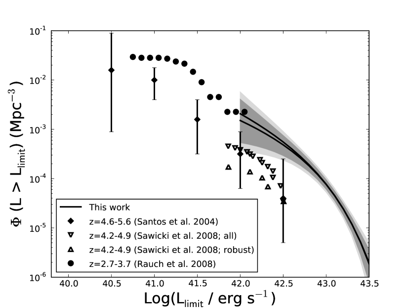
Figure 10.— Spectroscopic surveys measure the cumulative Ly$\alpha$ luminosity functions to very faint luminosities at $z\gtrsim 3$. These include a search for strongly lensed LAEs (Santos et al., 2004), a serendipitous survey (Sawicki et al., 2008), and a very long exposure with the Very Large Telescope (Rauch et al., 2008). The shaded area show the 68 and 95% confidence intervals from our LF fits, where, for simplicity we have taken the lower bounds from the 3 LAE LF and the upper bounds from the 6 LAE LF.

Figure 10 shows that the space density of LAEs spans a factor of several between these different measurements. Large statistical errors, coupled with differing analyses and a wide range of redshifts make it difficult to draw any conclusions. The highest space density of LAEs is found by Rauch et al. (2008), who also have the greatest sensitivity to low surface brightness emission. This could mean that they measure brighter luminosities by including more low surface brightness flux, and also that they are able to detect extended, luminous LAEs that other surveys would miss. However, where Rauch et al. overlap with our survey, the agreement is good. Lower densities are found at $z\sim 4-5$ by Santos et al. (2004) and Sawicki et al. (2008). At $L=10^{42.5}$ erg s^-1 , where they overlap with the wider, shallower search from Ouchi et al. (2008), the density of LAEs found by Santos et al. and Sawicki et al. is several times lower. The origin of this discrepancy is unclear. In short, statistical uncertainties make it difficult to determine if the faint end of the Ly$\alpha$ LF evolves at $z\sim 3-6$. Larger spectroscopic samples of faint LAEs are needed.

8.3. Comparison to UV-selected $i-$dropout samples

Surveys for LAEs have have often been motivated by the idea that line emission can be more easily detected than continuum when galaxies become very faint. This rationale is especially true for our spectroscopic search, which includes lines to fainter luminosities than most other Ly$\alpha$  searches. For example, at the median LAE luminosity in Table 2 ($L=10^{42.4}$ erg s^-1), a galaxy with rest Ly$\alpha$ equivalent width, $W_{0}$, larger than 190 Å will have $M_{UV}>-18$. At $z\sim 6$, this luminosity is beyond the limit of the $i-$dropout samples used to measure the UV-luminosty function (Bouwens et al., 2007). Likewise, at the $L=10^{42.0}$ erg s^-1 limit of our survey, a galaxy would need to have a rest equivalent width smaller than about 80 Å to have a continuum flux-density which is bright enough for inclusion in the $i-$dropout sample.

Of course, assessing whether LAE surveys are finding a significant population of previously unobserved galaxies is not straightforward. The Ly$\alpha$ equivalent width of star-forming galaxies displays a wide range of values, with a tail to quantities larger than $100-200$ Å (Shapley et al., 2003; Shimasaku et al., 2006; Gronwall et al., 2007; Stark et al., 2010, 2011). Consequently, a faint LAE could be the result of a low equivalent width emission from a UV-bright galaxy, or conversely, high equivalent width emission from an extremely faint galaxy. No obvious trends exist between Ly$\alpha$ luminosity and equivalent width (see Henry et al. 2010), although followup of UV-continuum selected $i-$dropouts shows that fainter continuum is correlated with stronger and more common Ly$\alpha$ emission (Stark et al., 2010, 2011). Ultimately, since Ly$\alpha$ equivalent width exhibits such a wide range of values, a statistical comparison with the ensemble of $i-$ dropout galaxies is most relevant.

To determine whether the LAEs in our sample are likely to be detectable as faint $i-$ dropouts, we generate a mock catalog of galaxies. Beginning with the UV-luminosity function of $z\sim 6$ $i-$ dropouts (Bouwens et al. 2007; $\phi^{*}=1.4\times 10^{-3}$ Mpc^-3, $M_{UV}^{*}=-20.24$, and $\alpha=-1.74$), we generate a sample of galaxies in a fixed volume, with UV-luminosities extending to $M_{UV}=-14.0$ (beyond the depth required for all LAEs in our survey to be detected in the continuum). A rest-frame Ly$\alpha$ equivalent width ($W_{0}$) is assigned to each galaxy in this volume, drawing from an exponential distribution with a maximum of $W_{0}=2000$ Å. Motivated by the observations shown in Stark et al. (2011; Figure 2), we adopt e-folding, or “characteristic” equivalent widths of 50 Å  for $M_{UV}>M_{UV}^{*}$, and 20 Å for $M_{UV}<M_{UV}^{*}$. These scale factors approximately reproduce the distribution of rest equivalent widths and the fraction of sources with equivalent width less than 25 Å. Since narrowband imaging surveys cannot detect LAEs with $W_{0}<25$ Å, galaxies which are given these low equivalent widths under our exponential parameterization are excluded from the Ly$\alpha$ LF. (Although we note that the Ly$\alpha$ LF is not strongly dependent upon this cutoff.) With each galaxy assigned an $M_{UV}$ and $W_{0}$, we calculate the Ly$\alpha$ luminosity of each $i-$dropout. To understand the impact of the current observational limit, we repeat this calculation including only galaxies brighter than $M_{UV}=-18$. The resulting simulated LFs are plotted in Figure 11, where they are compared to our measured constraints on the Ly$\alpha$ LF.

The simulated LFs shown in Figure 11 illustrate the importance of surveys for faint LAEs. With the equivalent width distributions chosen above, the Ly$\alpha$ LF simulated with only galaxies having $M_{UV}<-18$ (dashed curve) shows a significant deficit of LAEs relative to when the complete range of luminosities are included (solid curve). At the $L=10^{42}$ erg s^-1 limit of our survey, approximately 50% of LAEs should have $M_{UV}>-18$. Galaxies as faint as $M_{UV}\sim-16.5$ are needed to bring these two simulated LFs into agreement. This result clearly indicates that we have uncovered a population of galaxies whose continua are too faint to have been observed in the deepest space-based dropout surveys. On the other hand, the narrowband imaging surveys for brighter LAEs are not uncovering a previously unobserved population. Figure 11 shows that, brighter than $L=10^{42.5}$ erg s^-1, the Ly$\alpha$ luminosity function is dominated by galaxies with $M_{UV}<-18.0$.

Figure 11 shows that the simulated Ly$\alpha$ luminosity function falls short of observations at the bright end. A scale factor of 30 Å rather than 20 Å for the bright ($M_{UV}<M_{UV}^{*}$) $i-$ dropouts would bring the simulated luminosity function within the 68% confidence interval shown in Figure 11. A larger scale factor is not implausible, as the sample of bright $i-$dropouts targeted for spectroscopy by Stark et al. (2011) is not large enough to derive very precise constraints on the luminosity dependence of the Ly$\alpha$ equivalent width distribution. Additionally, it should be noted that the equivalent width distributions measured by Stark et al. (2011) are for galaxies that are selected as $i-$dropouts. The selection function for these galaxies is known to depend on Ly$\alpha$ equivalent widths (Bouwens et al., 2006; Stanway et al., 2007), so the “raw” equivalent width distributions presented by Stark et al. may not strictly represent the parent population of star-forming galaxies.

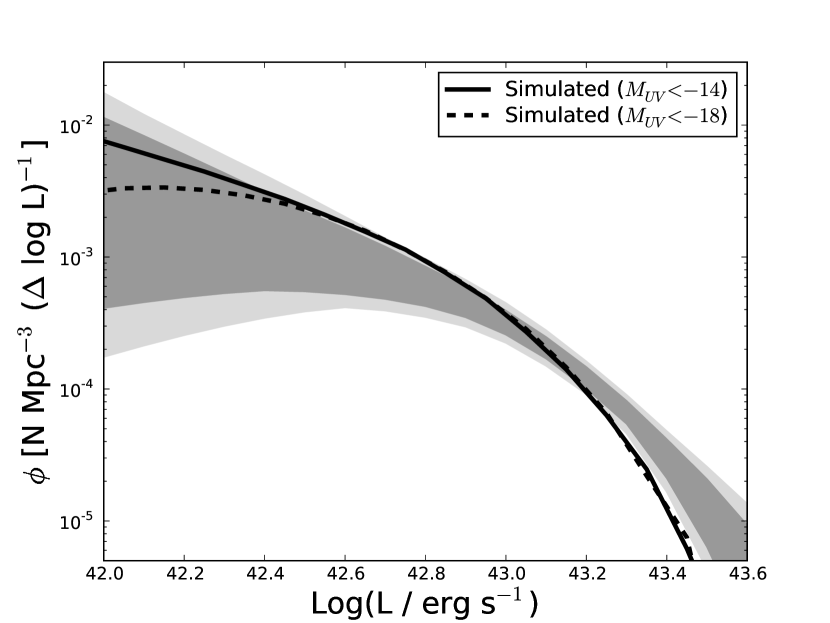
Figure 11.— Simulated Ly$\alpha$ LFs (solid and dashed curves) are compared to our LF constraints. The shaded regions show our 68 and 95% confidence limits. For simplicity, the lower bounds are taken from the 3 LAE LF and the upper bounds are taken from the 6 LAE LF. The simulated LFs are derived by including galaxies to very faint limits ($M_{UV}=-14$; solid), and also by limiting the simulation to luminosities that have been observed in the UDF and UDF-Parallels ($M_{UV}<-18$; dashed). The latter case turns over, representing an incompleteness to faint LAEs among the $i-$dropout samples. At the limit of our MNS survey (10⁴² erg s^-1), 50% of LAEs have UV luminosities fainter than the limit of current $i-$dropout samples.

One way to interpret the (incomplete) simulated Ly$\alpha$ luminosity function of galaxies with $M_{UV}<18$ is as a prediction of the Ly$\alpha$ LF that one could measure from spectroscopic followup of $i-$dropout galaxies (Jiang et al., 2011). However, correcting this LF to the “true” Ly$\alpha$ LF of all galaxies is not possible. We could speculate that the characteristic equivalent widths may be larger for galaxies with $M_{UV}>-18$ (following the trend of more prevalent Ly$\alpha$ emission among galaxies with fainter UV continuum luminosities). Under this scenario, the discrepancy between the simulated LFs shown in Figure 11 would be amplified, because the faint-end slope of the “true” LF (simulated to a realistic low-luminosity cutoff) would be even steeper. Since we cannot know the equivalent width distribution of the faint, continuum-undetected galaxies, only dedicated emission line surveys will be able to measure the faint-end slope of the Ly$\alpha$ LF.

8.4. Ly$\alpha$ line profiles

The transmission of Ly$\alpha$ photons is sensitive to the ionization state of the IGM, so the shape of the Ly$\alpha$ emission line profile may offer a measure of the changing neutral hydrogen fraction. In a more neutral IGM, the Gunn-Peterson Ly$\alpha$ damping-wing will lower the peak flux of the line, effectively broadening the emission and removing its asymmetric shape (Ouchi et al., 2010; Dayal et al., 2008).

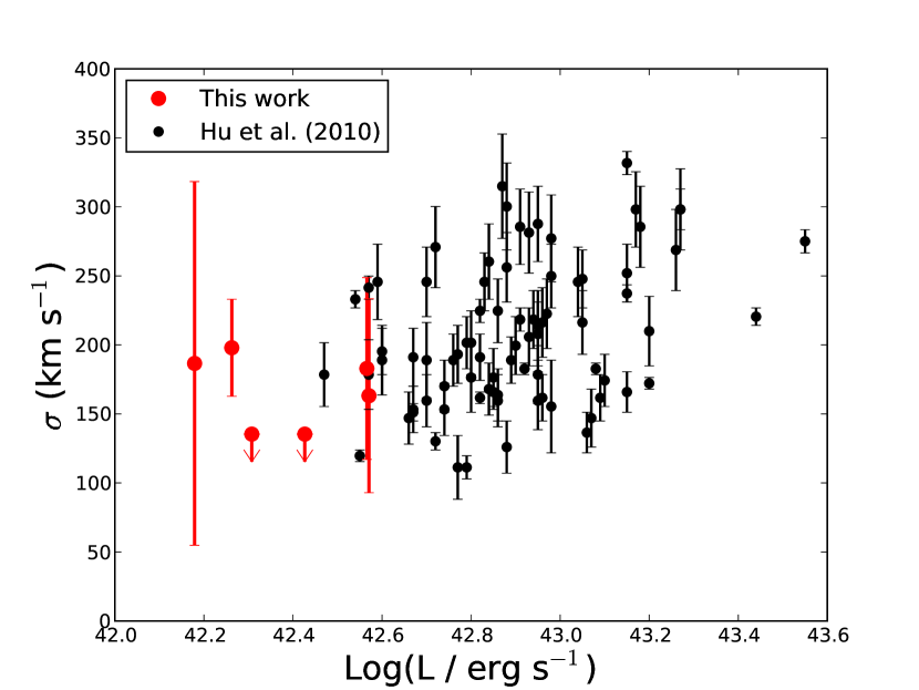
Figure 12.— The Ly$\alpha$ line width shows a positive correlation with luminosity. Here, $\sigma$ is determined in the same way for all LAEs: a truncated Gaussian is convolved with the instrumental resolution and fit to the observed line profile. Two objects have line profiles that are consistent with being unresolved, and for these we plot upper limits that correspond to the instrumental resolution.

Observational efforts have begun to search for a difference in Ly$\alpha$ profiles observed at redshifts 5.7 and 6.5 (Ouchi et al., 2010; Hu et al., 2010; Kashikawa et al., 2011), but the average line width is not significantly different between the two redshift bins. However, Hu et al. show that the Ly$\alpha$ line width displays a positive correlation with luminosity. In Figure 12 we combine our faint LAEs with the Hu et al. redshift 5.7 sample to extend the correlation to lower luminosities. As expected from an extrapolation of the brighter sources, our newly measured line widths are among the narrower values. The significance of the relation is improved: under the Spearman rank correlation test, the probability of the null hypothesis (no correlation) is decreased from $1.6\times 10^{-3}$ to $2.6\times 10^{-4}$ when our six faint LAEs are included. These probabilities, interpreted in the context of a Gaussian probability density function, increase the significance of the correlation from 3$\sigma$ to better than 3.5$\sigma$.

The luminosity dependence of the Ly$\alpha$ line-width has important implications for how the effects of reionization on the line profile are interpreted. Comparisons made at different redshifts should also be made at fixed luminosity. This luminosity dependence has not been accounted for when entire samples of redshift 5.7 and 6.5 LAEs have been stacked (Ouchi et al., 2010; Kashikawa et al., 2011). In a flux-limited sample, the redshift 6.5 LAEs will be, on average, more luminous. This could explain the observation that the redshift 6.5 line profiles are marginally broader than those at redshift 5.7.

The origins of the observed luminosity dependence are unclear. One explanation offered by Hu et al. (2010) is that the more luminous LAEs may simply be more massive, with intrinsically broader Ly$\alpha$ lines. Another possibility lies in the kinematics and conditions of the circumgalactic medium. While typical star-forming galaxies have redshifted Ly$\alpha$ emission and blueshifted P-Cygni absorption (Shapley et al., 2003; Steidel et al., 2010), rare cases are seen where blueshifted material emits rather than absorbs Ly$\alpha$ (Erb et al., 2010; McLinden et al., 2011). In these cases, the Ly$\alpha$ emission is both luminous, and broader than average. While Gunn-Peterson absorption will destroy blueshifted emission at redshift 5.7, the relative strength of the emission component at zero velocity may still induce a correlation between line width and luminosity. Measurements of LAE masses and systemic redshifts can distinguish these scenarios, but for reionization era galaxies, the required observations will remain challenging until the James Webb Space Telescope operates.

8.5. The contribution of faint LAEs to the hydrogen-ionizing background

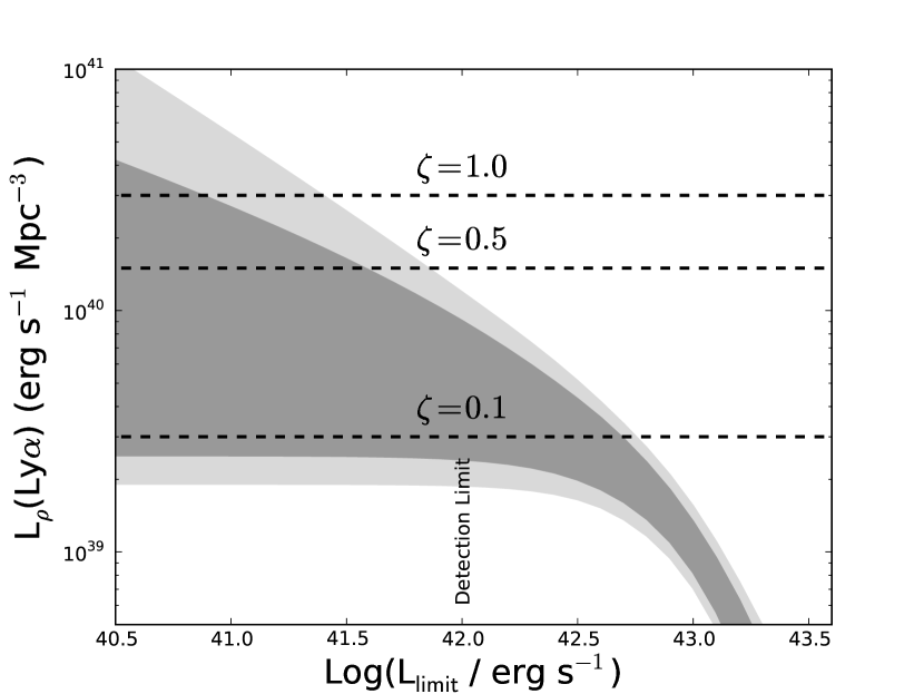
Figure 13.— Including galaxies fainter than those that we have observed increases the Ly$\alpha$ luminosity density, making it easier for galaxies to maintain an ionized IGM. Shaded regions show the 68 and 95% confidence limits on the Ly$\alpha$ luminosity density, as a function of the low-luminosity cutoff. To simplify, the upper bounds are taken from 6 LAE constraints and the lower bounds are taken from the 3 LAE constraints. The critical Ly$\alpha$ luminosity density required to maintain an ionized IGM at redshift 5.7 is $L_{\rho}(Ly\alpha)=\zeta\times 3.0\times 10^{40}$ erg s^-1 Mpc^-3. Horizontal lines mark $\zeta=0.1,0.5,$and 1.0.

At $z\sim 6$ the reionization of the intergalactic medium was complete, and the neutral hydrogen fraction in the IGM was negligible. Star-forming galaxies are usually assumed to produce the necessary ionizing background to prevent hydrogen recombination. However, observational constraints at redshifts 6 and higher have yet to demonstrate that galaxies produce the requisite ionizing background (Bunker et al., 2004, 2010; Bouwens et al., 2007, 2010a; Oesch et al., 2010). Often, galaxies which are too faint to be observed are invoked (Yan & Windhorst, 2004; Salvaterra et al., 2011; Finlator et al., 2011), extrapolating faint counts from brighter populations. In this paper, we address this shortcoming by detecting some objects from this hitherto undetected, postulated faint population (as demonstrated in §8.3).

In Figure 13 we show the cumulative Ly$\alpha$ luminosity density (as a function of the low-luminosity cutoff) allowed by our newly derived constraints. In order to determine whether LAEs can maintain an ionized IGM, we must infer an ionizing photon rate from the observed Ly$\alpha$ photons, and then address whether this ionization rate can balance the recombination rate in the IGM. This threshold depends on the escape of both Ly$\alpha$ and hydrogen-ionizing (LyC) photons ($f_{LyC}$ and $f_{Ly\alpha}$; Siana et al. 2010; Nestor et al. 2011; Hayes et al. 2011), as well as the clumpiness of ionized hydrogen in the IGM ($C\equiv\langle n^{2}_{\textrm{{H~{}II}}}\rangle/\langle n_{\textrm{{H~{}II}}}\rangle^{2}$). In Paper I and Paper II we renormalized these uncertain parameters to their best guess values and grouped them into a single parameter, $\zeta$. In this way, $\zeta=0.9$ when $C=6$, $f_{Lya}=0.5$, and $f_{LyC}=0.1$, and the critical Ly$\alpha$ luminosity density required to maintain an ionized IGM at redshift 5.7 is $L_{\rho}(Ly\alpha)=\zeta\times 3.0\times 10^{40}$ erg s^-1 Mpc^-3. Thresholds with $\zeta$ = 0.1, 0.5, and 1.0 are shown in Figure 13. This plot illustrates that, if $\zeta$ is among the smaller values of 0.1 to 0.5, it may be possible to maintain an ionized IGM with only the galaxies that we have observed. However, if $\zeta$ is larger, even fainter galaxies are needed and the faint-end slope must fall among the steeper values allowed by our data. As we pointed out in Paper II, when faint-end slopes are shallow ($\alpha\gtrsim-1.3$), the Ly$\alpha$ luminosity density grows very slowly when increasingly lower luminosities are included. Therefore, in the case of a shallow slope, it may be difficult for star-forming galaxies to reionize the IGM.

8.6. Properties of galactic building blocks at the end of reionization

In Paper II we compared our density of faint LAEs to that of local galaxies, estimating that we had found three or four sites of active star-formation per $L^{*}$ galaxy today. The implication of this result was that we had identified the building blocks of Milky-Way type galaxies. In this work, we have refined our faint-end slope measurements, and shown that the most-likely slope is shallower than the one we adopted in Paper II. As a result, the space density of LAEs that we have identified is about a factor of two smaller– $2\times 10^{-3}$ Mpc^-3. However, not all galaxies have Ly$\alpha$ emission. By comparison, the space density of observed $i-$dropouts is about 2-3 times higher than the LAE density that we observe. Furthermore, if $i-$dropouts were detected as faint as $M_{UV}=-16.5$ (our estimate of our faintest continuum luminosities from §8.3), their space density would be several times higher than the LAE density presented here. Since our LAEs belong to this class of postulated ultra-faint $i-$dropouts, we can infer that we have observed the building blocks of present day $L^{*}$ galaxies.

While it remains difficult to determine the physical properties of LAEs from their Ly$\alpha$ emission line alone, in Paper II we placed their properties in the larger context by comparison to other studies. For example, the angular correlation of the brighter LAEs presented in Ouchi et al. (2008, 2010) implies halo masses of $M=10^{11}-10^{12}~{}M_{\sun}$ at redshift 5.7. Presumably, the lower luminosity objects that we have found reside in less massive halos. Additionally, in Paper I we estimated SFRs as low as 1 to a few $M_{\sun}$ yr^-1 (if half of the Ly$\alpha$ photons escape the galaxy). If this star formation rate persists for a dynamical time scale of at least 50 Myr, then approximately $10^{8}$ $M_{\sun}$ of stars will have formed. These masses, SFRs, and redshifts are well matched to the predicted properties of the galaxies that enriched the IGM with metals (Oppenheimer et al., 2009; Martin et al., 2010).

As noted in §4, some of the LAEs have spatially resolved emission in our DEIMOS spectroscopy. This is not strictly surprising, as stacking of narrowband Ly$\alpha$ images at $z\sim 2-3$ has revealed that diffuse, extended Ly$\alpha$ emission is a generic component LAEs and LBGs alike (Steidel et al., 2011). Additionally, Rauch et al. (2008) find that, when exceptionally faint surface brightness limits are reached, a considerable fraction (40-70%) of redshift 3 LAEs are extended. Consequently, the observation that LAEs are compact in narrowband HST images (Bond et al., 2010; Finkelstein et al., 2011) does not imply that the Ly$\alpha$ emission region is small, but rather that the sensitivity to low surface brightness emission is insufficient in the space-based images. Further studies of extended Ly$\alpha$ emission in larger samples may help quantify the evolution of the circumgalactic medium at high-redshift.

9. Summary and Conclusions

We have measured the faint-end slope of the Ly$\alpha$ luminosity function at redshift 5.7, using Multi-slit Narrowband Spectroscopy (MNS) to identify faint emission lines. In Paper II (Dressler et al., 2011), we presented over 200 Ly$\alpha$ candidates and showed that a steep faint-end slope ($\alpha\sim-2$) was likely. Now, we have added spectroscopic followup to distinguish foreground line emitters and confirm LAEs. In this way, we have conclusively identified three, and tentatively identified three further LAEs. With these LAEs in hand, we develop the appropriate framework for deriving a luminosity function from blind-spectroscopic data, where the positions of galaxies within the search slit are not always known. The resulting Ly$\alpha$ LF has a faint-end slope of $-1.70^{+0.73}_{-0.57}$ ($-1.45^{+0.92}_{-0.70}$) when six (three) LAEs are used. When our spectroscopic followup in COSMOS and the LCIRS 15H field is complete, we can expect to identify around 40 LAEs, and improve the uncertainties on the LF measurements.

Studies of galaxies in the post-reionization era ($z\sim 4-6$) allow us to map the growth of young objects in an early universe. For the LAEs in our survey, we estimate SFRs of one to a few $M_{\sun}$ yr^-1, and a stellar mass of at least $10^{8}$ M_☉. In fact, these properties are matched to the masses, SFRs, and redshifts of galaxies that are thought to have enriched the IGM with metals (Oppenheimer et al., 2009; Martin et al., 2010).

By identifying some of the faintest galaxies ever observed at $z\sim 6$, we uncover objects that are important for the reionization of the IGM. In §8.5, we show that by extrapolating our faint-end slope measurement to low luminosities, it may be possible for LAEs to maintain an ionized IGM with our nominal assumptions about the escape fractions of LyC and Ly$\alpha$ photons ($f_{LyC}=0.1$ and $f_{Ly\alpha}=0.5$) and the clumpiness of the ionized hydrogen in the IGM ($C=6$). Nevertheless, the allowed Ly$\alpha$ luminosity density of sources brighter than $10^{41}$ erg s^-1 spans more than an order of magnitude. If the true value falls among the lower range allowed by our data, the escape fractions and clumping factor may need to be revised in order for galaxies to maintain an ionized IGM. Ultimately, this requirement may prove reasonable– the escape fractions and clumping factor are all uncertain. Future efforts to constrain these parameters, in parallel with improved measurements of galaxies will be needed if we are to conclusively determine, whether star-formation at $z\sim 6$ maintains the ionized IGM.

The LAEs presented here set a benchmark for comparison to higher redshift Ly$\alpha$ surveys that aim to measure the reionization of the IGM. By combining our line width measurements with those reported by Hu et al. (2010), we confirm that fainter LAEs have somewhat narrower line widths. Although the origin of this correlation is unclear, it must be taken into consideration when drawing conclusions about a (partially) neutral IGM from Ly$\alpha$ line profiles, since higher-redshift surveys will naturally be limited to more luminous LAEs. Furthermore, our measurement of the faint-end slope of the Ly$\alpha$ LF represents the first step towards measuring the faint-end evolution imparted by a neutral IGM. An MNS survey at redshift 6.5 could determine if the evolution observed at the bright-end (Kashikawa et al., 2006, 2011; Ouchi et al., 2010) persists at the faint-end. Such observations may constrain models that describe the propagation of ionized regions in a partially neutral IGM (e.g. Miralda-Escudé et al. 2000; Ciardi & Madau 2003; Furlanetto et al. 2006; Ono et al. 2011).

In summary, we have shown that spectroscopic searches for LAEs are able to uncover faint galaxies that cannot be observed by any other means. Measuring this population opens new windows to understanding the formation of young galaxies, and the enrichment and reionization of the IGM.

Appendix A A. Survey Completeness

To calculate the survey incompleteness for the IMACS search data, we take advantage of the fact that our emission line counts are well described by a power law between $F=10^{-16}$ and $10^{-17.2}$ erg s^-1 cm^-2 (see Figure 14) . This is easily understood, because we are summing the faint-end counts of (primarily) the constituent foreground populations– all of which are described by power-laws. Clearly, we can expect these counts to continue to rise to fainter emission line fluxes. Therefore, we predict the the number of all emission line galaxies by fitting power-law to the counts brighter than $10^{-17.2}$ erg s^-1 cm^-2 in both the COSMOS and 15H fields. (The sensitivity is the same for both fields, so we include the 15H field here to improve statistics.) This fit, illustrated in Figure 14 goes as $F^{-1.02\pm 0.12}$. The completeness of our survey– defined as the ratio of the observed counts to those predicted by our model– is plotted in Figure 14. A completeness fraction slightly greater than unity naturally arises when the power-law fit falls slightly below the data.

For comparison, we show the model adopted by Paper II, which was estimated from a modification to the completeness function presented in Paper I. The good agreement between the estimate in Paper II and the completeness calculated here indicates that no substantial revisions to the implications in Paper II are needed. Additionally, we note that the faintest bin that we consider in this paper contains many galaxies (42), so the Poisson noise on this calculation makes a negligible contribution to our error budget. Finally, while one might expect that the completeness to line emission is different for LAE candidates (without detected continuum) and foreground galaxies (with detected continuum), the faintest bins are dominated by LAE candidates, so it is reasonable to apply this incompleteness correction to the LAEs in our survey.

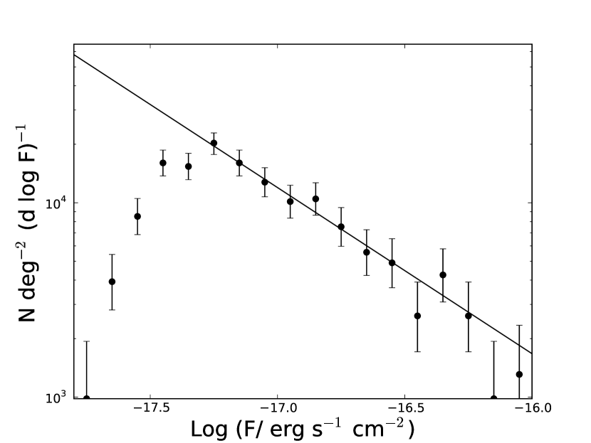
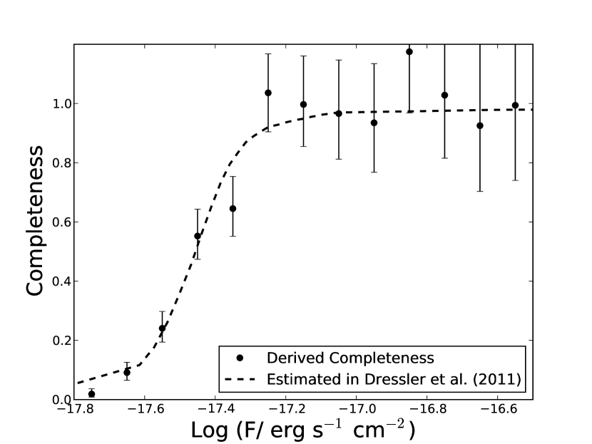
Figure 14.— The source counts of all emission line galaxies in our survey follow a power law, and are highly complete brighter than $F=10^{-17.2}$ erg s^-1 cm^-2. A fit to the counts above this threshold gives a power law index of $-1.02\pm 0.12$. Comparison of the observed counts to the extrapolated fit gives the survey completeness, shown on the right.

Appendix B B. Foreground Populations

In Paper II, we characterized the foreground H$\alpha$, [O III], and [O II] populations that comprise our sample of emission lines. Subtracting the foreground LFs estimated from the COSMOS field showed a significant excess of counts that suggested a steep rising slope ($\alpha\sim-2$) for the remaining galaxies that are likely LAEs. Additionally, an angular correlation of the Ly$\alpha$ candidates and [O II] emitters showed that fewer than 30% of the LAE candidates should be [O II]. Since even fewer should be H$\alpha$ and [O III], the implication is that approximately 100 LAEs may exist in the combined COSMOS and 15h survey fields. In this section, we show that the foreground number counts in COSMOS are indeed higher than what we adopted in Paper II, consistent with our preference for a slightly shallower faint-end slope for the Ly$\alpha$ LF.

In §5 we identified foreground galaxies through two means: objects which are obvious foreground emitters in the search data, and objects which were initially LAE candidates in the search data, but are now spectroscopically or photometrically identified as foreground galaxies. The counts of the total foreground populations are listed in Table 3, and shown again, for reference in Table 6 where we compare these counts to the numbers predicted by the foreground luminosity functions used by Paper II. In each bin, the foreground galaxy counts that we have identified so far are similar to (often exceeding) the number predicted by foreground LFs. In addition, in §5 we showed that the results of our spectroscopic followup indicate that the unidentified LAE candidates (for which counts are also listed in Tables 3 and 6) are predominantly foreground galaxies. Consequently, we expect that when our spectroscopic followup is complete, the observed foregrounds will be higher than the model favored in Paper II. We estimate these counts in the same way that we calculated the inferred LAE counts in §5. The inferred foreground number counts are given for two cases, with the low (high) counts referring to the case of six (three) genuine LAEs in this paper.

Including the foreground galaxies inferred among the unidentified line emitters makes the case clear: the nominal “best estimate” foreground counts in Paper II were underestimated, at least for the COSMOS field. However, they remain within range of reasonable foreground LFs which we considered. An alternative model is shown in Table 6 where the faint-end slopes are all steeper by $1\sigma$ from their adopted values (see Paper II). These counts agree more closely with our expectation from followup spectroscopy. However, a model where all three foreground populations have steeper slopes by 1$\sigma$ is contrived. It is more probable that the number counts of one of the foreground populations has been significantly underestimated.

Table 6Foreground Number Counts

Flux	Identified Foregrounds	Unidentified	$N_{pred}$	Inferred (Low)	Inferred (High)	$N_{pred}$ (+ 1$\sigma$)
-17.47	19	22	23.0	38.9	42.0	33.6
-17.27	39	13	35.8	47.8	49.9	49.0
-17.07	33	9	30.0	38.2	40.8	38.3
-16.87	24	6	22.5	$\sim 30$	$\sim 30$	27.0
-16.67	14	2	16.5	$\sim 16$	$\sim 16$	18.5
-16.47	14	0	10.8	14	14	11.3
-16.27	13	0	6.2	13	13	6.3
-16.07	6	0	3.0	6	6	3.0
-15.87	2	0	1.4	2	2	1.4
-15.67	1	0	0.7	1	1	0.7

The breakdown of the spectroscopically identified foreground galaxies in Table 4 suggests that H$\beta$ emitters are the cause of the larger foreground counts. In Dressler et al. (2011), this foreground population was not explicitly considered. It was, however, implicitly included with the [O III] population. When foreground emission line galaxies are detected through narrowband imaging, broad-band colors are typically used to identify the approximate redshift and probable line (Takahashi et al., 2007; Ly et al., 2007; Shioya et al., 2008). Not only does this mean that the [O III] catalog will contain some H$\beta$ emitters; an H$\alpha$ catalog may be contaminated by [S II] 6716, 6730 Å emitting galaxies. In practice, spectroscopic followup of bright emission lines from narrowband imaging samples has shown that contamination of this form is rare (Ly et al. 2007 find 16 [O III] emitters for only two H$\beta$ emitters). Even if this contamination were significant, the overall [O III] + H$\beta$ luminosity function should be sufficient to allow for an accounting of the total foreground populations at the bright end, as we did in Paper II.

Our spectroscopic followup observations, which included known foreground objects as slit-mask filler, provide strong evidence that H$\beta$ emitters in COSMOS play a more predominant role than we assumed in Paper II. In total, we have identified 15 [O III]  and 21 H$\beta$ emitters. The distributions of their fluxes are shown in Figure 15, where, relative to the numbers of [O III] emitters, an excess of H$\beta$ emitters fainter than about $8\times 10^{-18}$ erg s^-1 cm^-2 is observed.

One way to interpret the excess of faint H$\beta$ (relative to [O III]) emitters is as an indication that the faint-end of the H$\beta$ LF is significantly steeper than the [O III] LF. This would be the case if fainter [O III] emitters have progressively lower [O III]/H$\beta$ ratios. Since [O III]/H$\beta$ is strongly correlated with the R23 ({[O III]+ [O II]}/H$\beta$; Pagel et al. 1979) metallicity diagnostic, low [O III]/H$\beta$ ratios could be an indication of low oxygen abundance (when galaxies are on the lower-branch of R23). In practice, however, even the lowest metallicity galaxies observed at $z<1$ have high [O III]/H$\beta$ ratios (larger than three; Salzer et al. 2005; Kakazu et al. 2007). The [O III]/H$\beta$ ratios that we measure in our DEIMOS observations are similarly high. This means that it is difficult to interpret the excess H$\beta$ counts as an indication of low-metallicity galaxies.

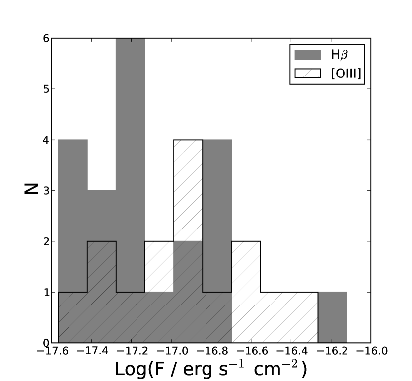
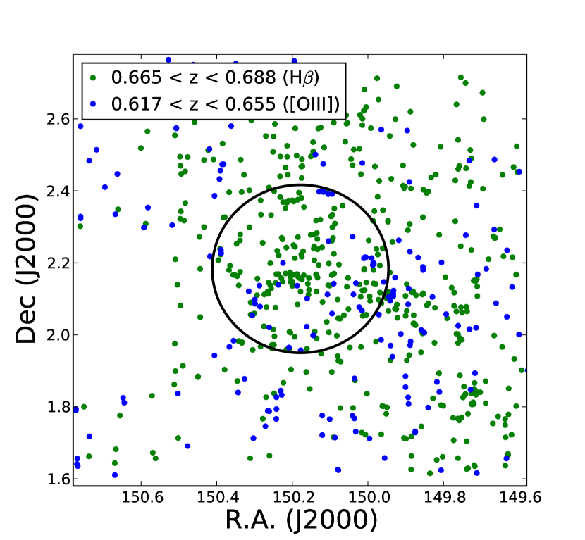
Figure 15.— Left– Spectroscopically confirmed H$\beta$ emitters outnumber [O III] emitters at faint fluxes. Right- The zCOSMOS (bright) spectroscopic catalog (Lilly et al., 2007) contains a significantly higher density of galaxies at $z\sim 0.68$ than at $z\sim 0.63$. Objects are shown for the redshift windows that correspond to H$\beta$ and [O III]$\lambda\lambda$4959, 5007 in our survey, although the latter volume is 50% larger. The footprint of our IMACS field is shown by the black circle. Within this region, there are four times as many galaxies at $z\sim 0.68$ than at $z\sim 0.63$, implying a volume density six times higher. We note that the coverage of zCOSMOS is not uniform over the regions shown here, but the relative numbers of the green and blue points should be unaffected.

A more probable explanation for the H$\beta$ emitters is that we have observed an overdensity at $z\sim 0.68$. In Figure 15, we use the zCOSMOS (bright) catalog of spectroscopic redshifts (Lilly et al., 2007) to show the spatial distributions of galaxies in the redshift windows that corresponds to H$\beta$ and [O III]$\lambda\lambda$4959, 5007. Even though the volume at the “[O III] redshift” is 50% larger than at the “H$\beta$ redshift”, the full zCOSMOS catalog contains 2.5 times as many galaxies in the latter redshift window. Within the footprint of our IMACS field (see Figure 15, right), this excess density is amplified, with a factor of four more galaxies in the redshift window at $z\sim 0.68$ than at $z\sim 0.63$. The excess of faint H$\beta$ emitters in Figure 15 (left) is easily explained by this overdensity, which is most apparent at luminosities fainter than the knee of the H$\beta$ LF. Therefore, the COSMOS foreground counts at faint fluxes are indeed higher than the model adopted in Paper II.

This increase over our previous estimates of the foreground populations in COSMOS does not erase our signal from LAEs. Although we find a slightly shallower slope ($-1.7$ as opposed to $-2.0$), these results are consistent, as $\alpha=-2.0$ falls within the 68% confidence interval that we present in this paper. Further followup spectroscopy (including our 15H field) will constrain the faint-end of the Ly$\alpha$ LF more tightly and simultaneously measure the faint foreground populations.

References

- Bertin & Arnouts (1996) Bertin, E., & Arnouts, S. 1996, A&AS 117, 393
- Bond et al. (2010) Bond, N. A., Feldmeier, J. J., Matković, A., Gronwall, C., Ciardullo, R., Gawiser, E. 2010, ApJ, 716, 200L
- Bouwens et al. (2004) Bouwens, R. J., Illingworth, G. D., Blakeslee, J. P., Broadhurst, T. J., & Franx, M. 2004, ApJ, 611, 1L
- Bouwens et al. (2006) Bouwens, R. J., Illingworth, G. D., Blakeslee, J. P., & Franx, M. 2006, ApJ, 653, 53
- Bouwens et al. (2007) Bouwens, R. J., Illingworth, G. D., Franx, M., & Ford, H. 2007, ApJ, 670, 928
- Bouwens et al. (2009) Bouwens, R. J., Illingworth, G. D., Franx, M., Chary, R.-R., Meurer, G.-R., Conselice, C. J., Ford, H., Giavalisco, M., & van Dokkum, P. 2009, ApJ, 705, 936
- Bouwens et al. (2010a) Bouwens, R. J., Illingworth, G. D., Oesch, P. A., Stiavelli, M., van Dokkum, P., Trenti, M., Magee, D., Labbé, I. Franx, M., Carollo, C. M., & Gonzalez, V. 2010, ApJ, 709, 133L
- Bouwens et al. (2010b) Bouwens, R. J., Illingworth, G. D., Oesch, P. A., Trenti, M., Stiavelli, M., Carollo, C. M., Franx, M., van Dokkum, P. G. Labbé, I., & Magee, D. 2010, ApJ, 708, 69L
- Bunker et al. (2004) Bunker, A. J., Stanway, E. R., Ellis, R. S., McMahon, R. G., MNRAS, 355, 374
- Bunker et al. (2010) Bunker, A. J., Wilkins, S., Ellis, R. S., Stark, D. P., Lorenzoni, S., Chiu, K., Lacy, M., Jarvis, M. J., Hickey, S. 2010, MNRAS, 409, 855
- Cassata et al. (2011) Cassata, P., et al. 2011, A&A, 525, 143
- Ciardi & Madau (2003) Ciardi, B., & Madau, P. 2003, ApJ, 596,
- Dayal et al. (2008) Dayal, P., Ferrara, A., & Gallerani, S. 2008, MNRAS, 389, 1683
- Dijkstra et al. (2007a) Dijkstra, M., Lidz, A., & Wyithe, J. S. B. 2007, MNRAS, 377, 1175
- Dijkstra et al. (2007b) Dijkstra, M., Wyithe, J. S. B., & Haiman, Z. 2007b, MNRAS, 379, 253
- Dressler et al. (2006) Dressler, A. D., Hare, T., Bigelow, B. C., Osip, D. J., 2006, SPIE, 6269, 13
- Dressler et al. (2011) Dressler, A., Martin, C. L., Henry, A. L., McCarthy, P., & Sawicki, M. 2011, submitted
- Dunlop et al. (2011) Dunlop, J. S., McLure, R. J., Robertson, B. E., Ellis, R. S., Stark, D. P., Cirasuolo, M., & de Ravel, L. 2011, arXiv:1102+5005
- Erb et al. (2010) Erb, D. K., Pettini, M., Shapley, A. E., Steidel, C. C., Law, D. R., & Reddy, N. 2010, ApJ, 719, 1168
- Faber et al. (2003) Faber, S. M., et al. 2003, SPIE, 4841, 1657
- Ferguson et al. (2004) Ferguson, H. C., et al. 2004, ApJ, 600, 107L
- Finkelstein et al. (2010) Finkelstein, S. L., Papovich, C., Giavalisco, M., Reddy, N. A., Ferguson, H. C., Koekemoer, A. M., & Dickinson, M. 2010, ApJ, 719, 1250
- Finkelstein et al. (2011) Finkelstein, S. L., et al. 2011, ApJ, 735, 5
- Finlator et al. (2011) Finlator, K., Davé, R., & Özel, F. 2011, arXiv:1106.4321
- Furlanetto et al. (2006) Furlanetto, S. R., Zaldarriaga, M., & Hernquist, L. 2006, MNRAS, 365, 1012
- Gronwall et al. (2007) Gronwall, C., et al. 2007, ApJ, 667, 79
- Gronwall et al. (2011) Gronwall, C., Bond, N. A., Ciardullo, R., Gawiser, E., Altmann, M., Blanc, G. A., & Feldmeier, J. J. 2011, arXiv:1005.3006
- Haiman & Cen (2005) Haiman, Z., & Cen, R. 2005, ApJ, 623, 627
- Hayes et al. (2011) Hayes, M., Schaerer, D., Östlin, G., Mas-Hesse, J. M., Atek, H., & Kunth, D. 2011, ApJ, 730, 8
- Henry et al. (2009) Henry, A. L., Siana, B., Malkan, M. A., Ashby, M. L. N., Bridge, C. R., Chary, R.-R., Colbert, J. W., Giavalisco, M., Teplitz, H. I., & McCarthy, P. J. 2009, ApJ, 697, 1128
- Henry et al. (2010) Henry, A. L., Martin, C. L., Dressler, A., McCarthy, P. J., & Sawicki, M. 2010, ApJ, 719, 658
- Hu et al. (2010) Hu, E. M., Cowie, L. L., Barger, A. J., Capak, P., Kakazu, Y., & Trouille, L. 2010, ApJ, 725, 394
- Ilbert et al. (2009) Ilbert, O., et al. 2009, ApJ, 690, 1236
- Jiang et al. (2011) Jiang, L., Egami, E., Kashikawa, N., Walth, G., Matsuda, Y., Shimasaku, K., Nagoo, T., Ota, K., & Ouchi, M. 2011, arXiv:1109.0023
- Kakazu et al. (2007) Kakazu, Y., Cowie, L., & Hu, E. M. 2007, ApJ, 688, 853
- Kashikawa et al. (2006) Kashikawa, N., et al. 2006, ApJ, 648, 7
- Kashikawa et al. (2011) Kashikawa, N., et al. 2011, ApJ, 734, 119
- Koekemoer et al. (2007) Koekemoer, A., et al. 2007, ApJS, 172, 196
- Lilly et al. (2007) Lilly, S. J., et al. 2007, ApJS, 172, 70
- Ly et al. (2007) Ly, C., Malkan, M. A., Kashikawa, N., Shimasaku, K., Doi, M., Nago, T., Iye, M., Kodama, T., Morokuma, T., & Motohara, K. 2007, ApJ, 657, 738
- Malhotra et al. (2011) Malhotra, S., Rhoads, J. E., Finkelstein, S. L., Hathi, N., Nilsson, K., McLinden, E., & Pirzkal, N. 2011, arXiv:1106.2816
- Martin et al. (2008) Martin, C. L., Sawicki, M., Dressler, A., & McCarthy, P. 2008, ApJ, 679, 942
- Martin et al. (2010) Martin , C. L., Scannapieco, E., Ellison, S. L., Hennawi, J. F., Djorgovski, S. G., & Fornier, A. P. 2010, ApJ, 721, 174
- Massey & Gronwall (1990) Massey, P. & Gronwall, C. 1990, ApJ, 358, 344
- Marzke et al. (1999) Marzke, R. O., et al. 1999, in ASP Conf. Ser. 191, in Photometric Redshifts and the Detection of High Redshift Galaxies, ed. R. Weymann et al. (San Francisco, CA: ASP), 148
- McLinden et al. (2011) McLinden, E. M., et al. 2011, ApJ, 730, 136
- McQuinn et al. (2007) McQuinn, M., Hernquist, L., Zaldarriaga, M., & Dutta, S. 2007, MNRAS, 381, 75
- Miralda-Escudé et al. (2000) Miralda-Escudé, J., Haenelt, M., & Rees, M. J. 2000, ApJ, 530, 1
- Murayama et al. (2007) Murayama, T., et al. ApJS, 172, 523
- Nestor et al. (2011) Nestor, D. B., Shapley, A. E., Stiedel, C. C., & Siana, B. 2011, ApJ, 736, 18
- Oesch et al. (2010) Oesch, P. A., Bouwens, R. J., Illingworth, G. D., Carollo, C. M., Franx, M., Labbé, I., Magee, D., Stiavelli, M., Trenti, M., & van Dokkum, P. G. 2010, 709, 16L
- Oke (1990) Oke, J. B. 1990, AJ, 99, 1621
- Ono et al. (2011) Ono, Y., et al. 2011, arXiv:1107.3159
- Oppenheimer et al. (2009) Oppenheimer, B. D., Davé, R., & Finlator, K. 2009, MNRAS, 396, 729
- Ouchi et al. (2008) Ouchi, M., et al. 2008, ApJS, 176, 301
- Ouchi et al. (2010) Ouchi, M., et al. 2010, ApJ, 723, 869
- Pagel et al. (1979) Pagel, B. E. J., Edmunds, M. G., Blackwell, D. E., Chun, M. S., & Smith, G. 1979, MNRAS, 189, 95
- Rauch et al. (2008) Rauch, M., et al. 2008, ApJ, 681, 856
- Reddy et al. (2008) Reddy, N. A., Steidel, C. C., Pettini, M., Adelberger, K. L., Shapley, A. E., Erb, D., & Dickinson, M. 2008, ApJS, 175, 48
- Rhoads et al. (2000) Rhoads, J. E., Malhotra, S., Dey, A., Stern, D., Spinrad, H., Jannuzi, B. T. 2000, ApJ, 545, 85L
- Salvaterra et al. (2011) Salvaterra, R., Ferrara, A., & Dayal, P. 2011, MNRAS, 414, 847
- Salzer et al. (2005) Salzer, J. J., Lee, J. C., Melbourne, J., Hinz, J. L., Alonso-Herroro, A., & Jangren, A. 2005, 624, 661
- Sandage, Tammann, & Yahil (1979) Sandage, A., Tammann, G. A., & Yahil, A. 1979, ApJ, 232, 352
- Santos et al. (2004) Santos, M. R., Ellis, R. S., Kneib, J.-P., Richard, J., Kuijken, K. 2004, ApJ, 606, 683
- Sawicki et al. (2008) Sawicki, M., Lemaux, B. C., Guhathakurta, P., Kirby, E. N., Konidaris, N. P., Martin, C. L., Cooper, M. C., Koo, D. C., Newman, J. A., & Weiner, B. J. 2008, ApJ, 687, 884
- Schenker et al. (2011) Schenker, M. A. , Stark, D. P., Ellis, R. S., Robertson, B. E., Dunlop, J. S., McLure, R. J., Kneib, J.-P., & Richard, J. 2011, arXiv:1107.1261
- Scoville et al. (2007) Scoville, N., et al. 2007, ApJS, 172, 1
- Shapley et al. (2003) Shapley, A. E., Steidel, C. C., Pettini, M., & Adelberger, K. L. 2003, ApJ, 588, 65
- Shimasaku et al. (2006) Shimasaku, K., et al. 2006, PASJ, 58, 313
- Shioya et al. (2008) Shioya, Y., et al. 2008, ApJS, 175 128
- Siana et al. (2010) Siana, B., et al. 2010, ApJ, 723, 241
- Stanway et al. (2007) Stanway, E. R. Bunker, A. J., Glazebrook, K., Abraham, R. G., Rhoads, J., Malhotra, S., Crampton, D., Colless, M., & Chiu, K. 2007, MNRAS, 376, 727
- Stark et al. (2010) Stark, D. P., Ellis, R. S., Chiu, K., Ouchi, M., & Bunker, A. 2010, MNRAS, 408, 1628
- Stark et al. (2011) Stark, D. P., Ellis, R. S., & Ouchi, M. 2011, ApJ, 728, 2L
- Steidel et al. (2010) Steidel, C. C., Erb, D. K., Shapley, A. E., Pettini, M., Reddy, N., Bogosavljević, M. Rudie, G., & Rakic, O. 2010, ApJ, 717, 289
- Steidel et al. (2011) Steidel, C. C., Bogosavljević, M., Shapley, A. E., Kollmeier, J. A., Reddy, N. A., Erb, D. K., & Pettini, M. 2011, arXiv:1101.2204
- Stubbs & Tonry (2006) Stubbs, C. W., & Tonry, J. L. 2006, ApJ, 635, 1006
- Takahashi et al. (2007) Takahashi, M. I., et al. 2004, ApJS, 172, 456
- Taniguchi et al. (2009) Taniguchi, Y., et al. 2009, ApJ, 701, 915
- Trenti & Stiavelli (2009) Trenti, M., & Stiavelli, M. 2009, ApJ694, 879
- Yan & Windhorst (2004) Yan, H., & Windhorst, R. A. 2004, ApJ, 600, 1L