Luminosity Discrepancy in the Equal-Mass, Pre–Main Sequence Eclipsing Binary Par 1802: Non-Coevality or Tidal Heating?

Abstract

Parenago 1802 (catalog ), a member of the $\sim$1 Myr Orion Nebula Cluster, is a double-lined, detached eclipsing binary in a 4.674 d orbit, with equal-mass components ($M_{2}/M_{1}$=0.985$\pm$0.029). Here we present extensive $VI_{C}$JHK_S light curves spanning $\sim$15 yr, as well as a Keck/HIRES optical spectrum. The light curves evince a third light source that is variable with a period of 0.73 d, and is also manifested in the high-resolution spectrum, strongly indicating the presence of a third star in the system, probably a rapidly rotating classical T Tauri star. We incorporate this third light into our radial velocity and light curve modeling of the eclipsing pair, measuring accurate masses ($M_{1}$=0.391$\pm$0.032, $M_{2}$=0.385$\pm$0.032 M_☉), radii ($R_{1}$=1.73$\pm$0.02, $R_{2}$=1.62$\pm$0.02 R_☉), and temperature ratio ($T_{\rm eff,1}/T_{\rm eff,2}$=1.0924$\pm$0.0017). Thus the radii of the eclipsing stars differ by 6.9$\pm$0.8%, the temperatures differ by 9.2$\pm$0.2%, and consequently the luminosities differ by 62$\pm$3%, despite having masses equal to within 3%. This could be indicative of an age difference of $\sim 3\times 10^{5}$ yr between the two eclipsing stars, perhaps a vestige of the binary formation history. We find that the eclipsing pair is in an orbit that has not yet fully circularized, $e$=0.0166$\pm$0.003. In addition, we measure the rotation rate of the eclipsing stars to be 4.629$\pm$0.006 d; they rotate slightly faster than their 4.674 d orbit. The non-zero eccentricity and super-synchronous rotation suggest that the eclipsing pair should be tidally interacting, so we calculate the tidal history of the system according to different tidal evolution theories. We find that tidal heating effects can explain the observed luminosity difference of the eclipsing pair, providing an alternative to the previously suggested age difference.

1 Introduction

The initial mass and chemical composition of newly formed stars are key factors in determining their evolutionary path. Multiple systems are commonly considered to be formed simultaneously from the same protostellar core, such that their components are assumed to be coeval and to have the same metallicity. Equal-mass components of binary systems—i.e., twins (e.g., Simon & Obbie, 2009)—are therefore expected to evolve following essentially the same evolutionary track.

Eclipsing binary (EB) systems are useful observational tools that render direct measurements of their components’ physical parameters, independent of theoretical models and distance determination, against which theoretical evolutionary models can be tested. There are a few tens of pre–main-sequence (PMS) systems for which the dynamical stellar masses are measured (Mathieu et al., 2007, and references therein); EBs however are the only ones that allow for the direct measurement of the radii of the components. EBs are rare, because their orbits have to be oriented such that we see the components eclipse. For PMS, low-mass EBs, where both components have masses below 1.5 M_☉, there are only seven such systems reported in the literature: ASAS J052821+0338.5 (Stempels et al., 2008); RX J0529.4+0041 (Covino et al., 2000, 2004); V1174 Ori (Stassun et al., 2004); MML 53 (Hebb et al., 2010); Parenago 1802 (Cargile et al., 2008; Stassun et al., 2008, and target of this study); JW 380 (Irwin et al., 2007), and 2M0535$-$05 (Stassun et al., 2006, 2007; Gómez Maqueo Chew et al., 2009). For the latter, the components are below the hydrogen-burning limit, i.e., they are brown dwarfs. For this particular system, the effective temperatures of the two bodies are observed to be reversed with the more massive brown dwarf appearing to be cooler. Similar to the approach we apply here for Par 1802, Heller et al. (2010) have explored the effects of tidal heating in that system.

The discovery of Par 1802 was previously presented, along with its radial velocity study that found the system to be an EB with a period of $\sim$4.67 d where both components have near equal masses, $M_{1}$ = 0.40$\pm$0.03 M_⊙ and $M_{2}$ = 0.39$\pm$0.03 M_⊙ (Cargile et al., 2008, hereafter Paper I). Par 1802, as a member of the Orion Nebula Cluster (ONC; Hillenbrand, 1997), is considered to have an age of $\sim$1 Myr (Paper I). A follow-up analysis which included the radial velocity curves and the $I_{C}$-band light curve found the components’ masses to be equal to within $\sim$2%, but their radii and effective temperatures to differ by $\sim$5–10% (Stassun et al., 2008, hereafter Paper II). They suggest that these disparate radii and temperatures are the result of a difference in age of a few hundred thousand years.

In this paper, we present new $VI_{C}$JHK_S light curves for Par 1802 as well as a newly acquired high-resolution optical spectrum (§2). The multi-band nature of our analyses (§3) allows us to probe the radiative properties of the system. The analysis includes an in-depth periodicity analysis of the light curves, which enables us to refine the orbital period for the binary and identify the rotation periods of its components (§3.1). We are also able to measure the presence of a third light source in the system (§3.2), through identification of a very short-period modulation in the light curves that definitively cannot be due to rotation of either of the eclipsing stars, through the analysis of an additional continuum contribution in the spectra, through analysis of third-light dilution in the light curves, and through analysis of the system’s broadband spectral energy distribution. We combine these analyses into a comprehensive, global model of the EB’s fundamental orbital and physical properties (§4), along with formal and heuristic uncertainties (obtained from a direct $\chi^{2}$ mapping of the parameter space) in these parameters. Par 1802 is found to be a low-mass PMS EB with a nominal age of $\sim$1 Myr, comprising two equal-mass eclipsing stars of 0.39 M_☉ and a third similarly low-mass star, probably in a wide orbit, that is rapidly rotating and likely accreting (i.e., a Classical T Tauri star). The radii of the eclipsing pair differ by 6.9$\pm$0.8%, their effective temperatures differ by 9.2$\pm$0.2%, and consequently, their luminosities differ by 62$\pm$3%, despite their masses being equal to within 3%.

In §5, we discuss possible explanations for the large difference in luminosity of the eclipsing pair, including magnetic activity, non-coevality arising from mass-equalizing effects in the binary’s formation, and tidal heating arising from the binary’s past orbital evolution. The last two explanations appear plausible, with the latter predicting a possible misalignment of the stellar spin axes, which could be observable. We summarize our conclusions in §6.

2 Data

2.1 Photometric Observations

We present the light curves of Par 1802 in $V$ (with a total of 2286 data points), $I_{C}$ (3488), $J$ (564), $H$ (176) and $K_{S}$ (365). The detailed observing campaign is described in Table 1, and the individual measurements in each observed passband are given in Tables 2–6. The $I_{C}$ data cover the largest time span, from December 1994 to January 2009; it includes the previously published light curve (Paper II) and 1279 new data points obtained between March 2007 and January 2009. The $V$ light curve includes data obtained between January 2001 and January 2009 with the 0.9-m telescope at KPNO and with the SMARTS 0.9-m, 1.0-m and 1.3-m telescopes at CTIO. Using the ANDICAM instrument which allows for simultaneous optical and near-infrared imaging, Par 1802 was observed photometrically with the SMARTS 1.3-m telescope at CTIO between February 2005 and February 2008, constituting the entirety of the JHK_S light curves. We also observed Par 1802 in the $B$-band; however, the resulting light curve was not well-sampled and it is very noisy due to the photometric variability of the third star in the system (see below). Thus, we do not include the $B$-band in the rest of our analyses, except as a consistency check of our final solution.

Because the light curve data were obtained mostly in queue mode on a variety of instruments over a long period of time, individual exposure times varied depending on the instrument and observing conditions. Typically, however, the $VI_{C}$ light curve data were obtained with typical exposure times of 60 s. The observations in the near-infrared were made in sets of five dither positions for the $J$-band, and seven dither positions for the $HK_{S}$-bands, with total integration times of 150 s and 175 s, respectively.

The optical ($VI_{C}$) light curves were determined via ensemble differential PSF photometry (see Honeycutt (1992); Stassun et al. (1999, 2002); and references therein) using the full ensemble of other stars in the field view, which is typically several hundred stars, except in the ANDICAM data for which it is typically a few tens of stars. Thus the differential light curve solutions do not rely upon individual comparison stars, and the solutions are much more robust against CCD-wide systematics. Data from different seasons and/or instruments are placed onto a common photometric scale determined from this large ensemble of comparison stars. In addition, to allow for small systematic offsets from season to season or across instruments, we subtracted from each season’s light curve the median out-of-eclipse value, which is well determined because of the large number of data points in each light curve.

Differential photometry on the $JHK_{S}$ light curves followed the procedures in Gómez Maqueo Chew et al. (2009), using an aperture of 6 pixels, which corresponds to 1.5 times the typical FWHM of the images. In this case, the comparison star used for the $JHK_{S}$ light curves was Par 1810, chosen because it is present in all of the reduced images of Par 1802 and because it exhibits no variability in the $I_{C}$ and $V$ bands; furthermore, it is not listed as variable in the near-infrared variability study of the ONC by Carpenter et al. (2001). The typical uncertainty in the $VI_{C}$ light curves is $\sigma_{I}=0.01$ mag and $\sigma_{V}=0.025$ mag, the latter dominated by poor sky subtraction due to scattered light in the nebular background. The uncertainty in the produced JHK_S light curves is dominated by the systematic uncertainties in the sky background subtraction. The $JH$ bands have a similar scatter, $\sigma_{J}=\sigma_{H}=0.01$ mag; however, the interference pattern of the sky emission lines in the $K_{S}$ light curve is more significant making the scatter in this band larger, $\sigma_{K_{S}}=0.02$ mag. These uncertainties were estimated by calculating the standard deviation of the light curves, with the data during eclipses excluded and the periodic low-amplitude variability (see §3.1) subtracted.

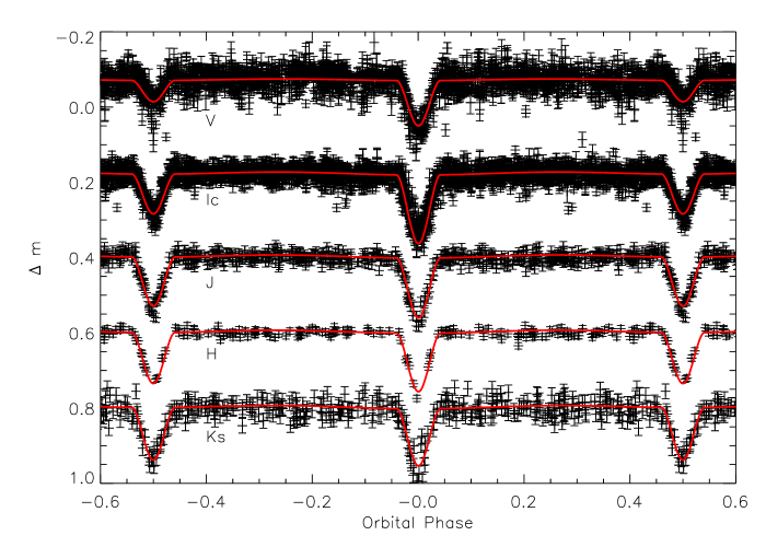
Figure 1: Observed and Modeled $VI_{C}$JHK_S Light Curves of Par 1802. We show the observed photometric light curves with their corresponding uncertainties as described in §2.1. The data have been folded over the binary’s orbital period and shifted in magnitude for easier visualization. The solid line represents the best RV+LC solution for Par 1802 (see §4 for a detailed description of the modeling procedure, and see Table 10 for the physical parameters of the EB components and their orbit).

Fig. 1 shows the $VI_{C}$JHK_S light curves, including those published in Paper II. The data have been folded on the orbital period and each band has been offset for clarity. Each point is an individual observation and the solid line represents the model of our final light-curve solution (§4).

2.2 Spectroscopic Observations

We observed Par 1802 on the night of UT 2007 Oct 23 with the High Resolution Echelle Spectrometer (HIRES) on Keck-I. The exposure time was 900 s. We observed in the spectrograph’s “red” (HIRESr) configuration with an echelle angle of $-0.403$ and a cross-disperser angle of 1.703. We used the OG530 order-blocking filter and 1$\farcs$15$\times$7$\farcs$0 slit, and binned the chip during readout by 2 pixels in the dispersion direction. The resulting resolving power is $R\approx 34\,000$ per 3.7-pixel ($\sim 8.8$ km s^-1) FWHM resolution element. For the analyses discussed below, we used the 21 spectral orders from the “blue” and “green” CCD chips, covering the wavelength range $\lambda\lambda$5782–8757. ThAr arc lamp calibration exposures were obtained before and after the Par 1802 exposure, and sequences of bias and flat-field exposures were obtained at the end of the night. The data were processed using standard IRAF tasks and the MAKEE reduction package written for HIRES by T. Barlow, which includes optimal extraction of the orders as well as subtraction of the adjacent sky background. The signal-to-noise of the final spectrum is $\approx 70$ per resolution element.

In addition, we observed the late-type spectral standards (see Kirkpatrick et al., 1991), Gl 205 (M1) and Gl 251 (M3), at high signal-to-noise. These spectral types were chosen to match the inferred spectral types of the eclipsing components of Par 1802, based on the tomographic reconstruction analysis presented in Paper II. They were observed immediately before the Par 1802 exposure and used exactly the same instrumental configuration. We use these spectral standards below in our spectral decomposition analysis of the Par 1802 spectrum.

3 Analysis of Periodicity and Third Light

3.1 Periodicities in the Par 1802 Light Curves

We measure the timings of the eclipses in the $I_{C}$ light curve, which covers the longest time span, and are able to refine the ephemeris for Par 1802 by performing a least-square fit to the observed eclipse times. The individual eclipse times are measured by a least-squares fit of a Gaussian to those eclipses for which there are at least five data points and that include the minimum of each eclipse. Table 7 summarizes the measurements of the timings of the eclipses and their uncertainties. We find a best-fit orbital period of $P_{\rm orb}$=4.673903$\pm$0.000060 d, and epoch of primary minimum HJD₀=2454849.9008$\pm$0.0005 d, which we adopt throughout our analysis as the system’s ephemeris.

The eclipse times in Table 7 show an r.m.s. scatter of 28 min, which is much larger than the formal uncertainty of a few seconds on the individual timing measurements. We have checked for systematic trends in these timing variations on timescales of 1–20 yr, such as might be produced by reflex motion of the eclipsing pair induced by the third body in the system (see §3.2). However, we do not find evidence for systematic deviations of the eclipse times from the above simple linear ephemeris. Instead, we regard the scatter as more likely arising from spots on the stars, as manifested in the periodic light curve modulation from which we measure the stellar rotation period (see below). Surface spots can induce asymmetry in the eclipses and thus effectively shift the eclipse minima by a small fraction of the star crossing time (e.g., Torres & Ribas, 2002; Stassun et al., 2004). Indeed, the 28 min scatter in eclipse times corresponds to 0.0041 orbital phase, which is a small fraction ($\sim$4%) of the eclipse duration. As an example, adding a single cool spot (50% cooler than the photosphere) covering 1% of the primary star’s surface, can induce a shift of 20 min in the time of primary eclipse predicted by our non-spotted light curve model (see Sec. 4). Spots on the secondary eclipsing star, as well as the short-period light curve variations that we see from the rapidly rotating third star (see below), likely introduce additional shifts of comparable magnitude in the observed eclipse timings.

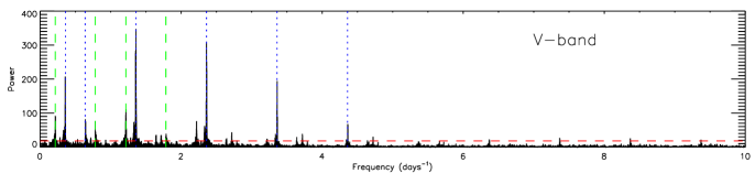
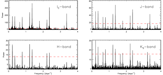
Figure 2: OFE $VI_{C}$JHK_S Lomb-Scargle Periodograms. The out-of-eclipse (OFE) light curves were searched for periodicities, as described in §3.1, identifying two independent periodic signals with frequencies of $\sim$0.216 and $\sim$1.36 d^-1, corresponding to periods of $P_{1}=4.629\pm 0.006$ and $P_{2}=0.7355\pm 0.0002$ d, respectively. Table 8 lists the identified periods in each observed passband with their corresponding uncertainties. The vertical, dashed lines on the top panel mark the frequency corresponding to $P_{1}$ and its aliases and beats; while the vertical, dotted lines correspond to the frequency of $P_{2}$ and its aliases and beats. The significance of the peaks is given by the horizontal, dashed line which denotes the 0.1% False-Alarm Probability (FAP); since most of the significant peaks are found between 0 and 4 d^-1, only the $V$-band periodogram is shown in its entirety. The out-of-eclipse $VI_{C}$JHK_S light curves folded over the two identified periods are presented in Fig. 3.

The $VI_{C}$JHK_S light curves corresponding to the out-of-eclipse (OFE) phases, i.e., all phases excluding those during the eclipses, are searched for periods between 0.1 and 20 d using the Lomb-Scargle periodogram technique (Scargle, 1982), which is well suited to our unevenly sampled data. The resulting periodograms (Fig. 2) show the power spectra in frequency units of d^-1 and present multiple strong peaks. These peaks represent a combination of one or more true independent signals and their aliases.

The amplitudes of the periodograms are normalized by the total variance of the data (Horne & Baliunas, 1986), yielding the appropriate statistical behavior which allows for the calculation of the false-alarm probability (FAP). To calculate the FAPs for each of the OFE light curves, a Monte Carlo bootstrapping method (e.g., Stassun et al., 1999) is applied; it does 1000 random combinations of the differential magnitudes, keeping the Julian Dates fixed in order to preserve the statistical characteristics of the data. The resulting 0.1% FAP level is indicated in the periodograms by the horizontal dashed line in Fig. 2. All periodogram peaks higher than the 0.1% FAP are considered to be due to real periodicity in our data; this includes the aliases and beats of any periodic signals.

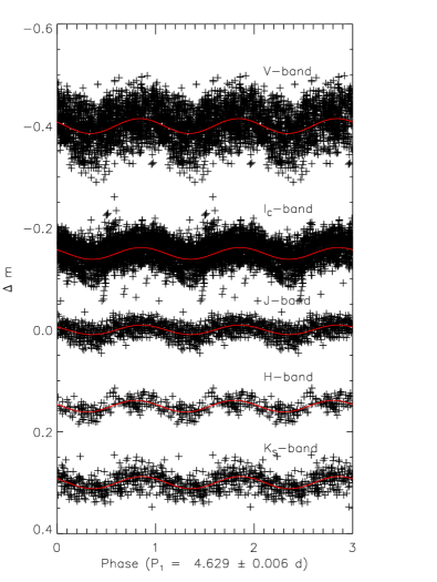
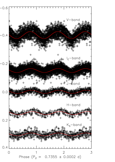
Figure 3: Low-Amplitude, Photometric Variability. The sinusoidal shape shown by the OFE light curves, folded over either of the two independent periods found in all observed passbands from the periodicity analysis (see Fig. 2 and Table 8), is characteristic of spot-induced, rotational modulation. The left-hand panel shows the $VI_{C}$JHK_S light curves folded over $P_{1}$ and displaced from zero for easier visualization. Superimposed is a sinusoid of period $P_{1}$ fitted to the data. In a similar way, the right-hand panel shows the same photometric OFE data folded over the shorter period, $P_{2}$, and its corresponding sinusoidal fit. The actual data points are repeated over each of the three phases shown. $P_{1}$ is attributed to the rotation period of the eclipsing components, and is consistent with their measured $v\sin{i}$ and radii; whereas $P_{2}$ is attributed to the stellar source of third light (see §3.2.4 for discussion on the third body). The amplitudes of this spot-induced variation at different passbands are obtained from the simultaneous fit of two sinusoids, and are given in Table 9.

To distinguish the periodogram peaks of the independent periods from their aliases, a sinusoid is fitted to each light curve and subtracted from the data in order to remove the periodicity corresponding to the strongest peaks in the periodograms. This filtering procedure allows us to identify in the OFE periodograms of all observed passbands two independent periods, $P_{1}$ = 4.629 $\pm$ 0.006 days and $P_{2}$ = 0.7355 $\pm$ 0.0002 days. These two periods are given by the mean of the individual period measurements in each band and their uncertainties are given by the standard deviation of the mean (see Table 8). When the OFE light curves are phased to either $P_{1}$ or $P_{2}$, they are characterized by having a sinusoidal low-amplitude variability which is indicative of stellar rotational modulation (e.g., Stassun et al., 1999). Fig. 3 shows on the left-hand side the OFE $VI_{C}$JHK_S light curves phased to $P_{1}$, and on the right-hand, the same data is phased to $P_{2}$. The periodograms of the OFE light curves after removing both sinusoidal signals are found to have peaks which are below the 0.1% FAP line, ensuring that the periodic signals are well fitted by sinusoids, that any deviation from true sinusoids is hidden within the scatter of the data, and that the other strong peaks in the periodograms are aliases or beats of these two periodic signals.

When we assess in detail the significant peaks in the periodograms of the OFE light curves, we find multiple-peaked structures due to the finite sampling of the data. The peaks corresponding to $P_{1}$ and its aliases, attributed to the one-day sampling of the light curves, are indicated in Fig. 2 by the vertical dashed lines; while $P_{2}$ and its one-day aliases are marked by the vertical dotted lines. We also find at each significant period that there is a finely spaced three-peaked structure, which is confirmed to arise from the seasonal (i.e., one-year) sampling of the data (see Appendix A).

$P_{1}$ is close to the orbital period of the binary ($P_{\rm orb}$ = 4.673903$\pm$0.000060 d), but is significantly different at a 7-$\sigma$ level. In order to better understand $P_{1}$, we search for periodicities in the residuals ($O-C$) of the EB modeling such that any period due to the EB nature of the system would be removed from the periodograms. We are able to again identify both $P_{1}$ and $P_{2}$ in the $O-C$ periodograms of all observed passbands. Table 8 describes in detail both identified periods in each observed light curve with their uncertainty, determined via a post-mortem analysis (Schwarzenberg-Czerny, 1991), for all of the OFE and $O-C$ periodograms. We are able to verify that we have sufficient frequency resolution to distinguish $P_{1}$ from $P_{\rm orb}$ (see Appendix A). Thus, we conclude that $P_{1}$ is not due to orbital effects, and in particular, $P_{1}$ significantly differs from $P_{\rm orb}$. If the photometric, low-amplitude variability is caused by surface spots rotating in and out of view on one or both of the binary components, the difference between $P_{1}$ and $P_{\rm orb}$ indicates that the rotation of the stars is not fully synchronized to the orbital motion (see below).

We measured the amplitudes of the periodic variability for both $P_{1}$ and $P_{2}$ by simultaneously fitting two sinusoids with these periods to each light curve. The measured amplitudes of the $P_{1}$ and $P_{2}$ signals are similar, $\sim$0.01–0.02 mag, and moreover they decrease with increasing wavelength as expected for spot modulated variability (see Table 9). The error of the amplitudes from the fit of the data to the double-sinusoid is $<$ 0.03% in all bands.

The 4.629-d period ($P_{1}$) is consistent with the spectroscopically determined $v\sin{i}$ (17$\pm$2 and 14$\pm$3 km s^-1 for the primary and secondary components, respectively; Paper II) and the directly measured radii of the EB components, $P_{\rm rot,1}/P_{\rm rot,2}=0.88\pm 0.22$. Thus we adopt $P_{1}$ as their rotational periods $P_{\rm rot}$. We defer to §5.3 a full discussion of $P_{\rm rot}$ in the context of tidal evolution theory, but we note here that it is reasonable to assign the same rotation period to both eclipsing stars. As the eclipsing components are being driven by tides toward synchronization to their orbital motion, radial contraction is changing the spin rates via conservation of angular momentum. In addition, Zahn & Bouchet (1989) and Khaliullin & Khaliullina (2011) both argue that the orbital period of Par 1802 is small enough for circularization and synchronization to occur prior to the arrival on the main sequence. As such, the assignment of $P_{1}$ as the rotational period of both eclipsing components is reasonable. It is consistent with the independently determined observational constraints (i.e., $v\sin i$, $R_{1}$, and $R_{2}$), and moreover, it represents the conservative choice in our discussion of the tidal heating effects in §5.3.

The short period ($P_{2}$) is too fast to be due to rotation of either of the binary components; with measured radii of $\sim$1.7 R_☉, $P_{2}$ would imply $v\sin{i}\approx 115$ km s^-1, which is entirely inconsistent with the measured $v\sin{i}$ of the eclipsing components. This periodicity, which as discussed above is clearly present at all epochs of our light curves spanning 15 yr, strongly suggests the presence of a rapidly rotating third star. Indeed, there is ample additional evidence for the existence of a third star in the Par 1802 system, as we now discuss.

3.2 Characterization of a Third Stellar Component in Par 1802 

In this section, we present additional evidence for a third stellar component in the Par 1802 system, which includes: (1) the presence of a featureless continuum in the high-resolution spectrum of Par 1802 that dilutes the spectral features of the eclipsing components, (2) the presence of “third light” in the multi-band light curves which dilutes the eclipse depths, and (3) the overall spectral energy distribution of Par 1802, which is best matched by a third stellar photosphere plus blue excess in addition to the photospheres of the two eclipsing components. The properties of the third stellar component are then used to refine the physical parameters that we determine for the EB pair in §4.

3.2.1 High-Resolution Spectroscopic Decomposition

In Paper II, we applied the method of tomographic decomposition on the same multi-epoch spectra from which we determined the EB radial velocities to recover the spectra of the individual stars, and found in that analysis that the reconstructed spectra of the primary and secondary are compatible with spectral types of M1V and M3V, respectively, implying $T_{\rm eff}$_,1=3705 K and $T_{\rm eff}$_,2=3415 K (from the spectral-type–$T_{\rm eff}$ scale of Luhman, 1999), which are consistent with the $T_{\rm eff}$’s determined from the light curve modeling of the system (see §4). In addition, a detailed analysis of the relative line depths of the reconstructed spectra made it possible to estimate their monochromatic luminosity ratio, which was found to be $L_{\rm 1}/L_{\rm 2}\approx 1.75$ for the wavelength region around 7000Å. This luminosity ratio was also shown in Paper II to be consistent with the $T_{\rm eff}$ ratio and radii ratio measured from the light curve modeling of the system.

In that analysis, we found that the photospheric absorption lines appeared diluted, but we attributed this to poor background subtraction because the spectra used in Paper II were obtained with a fiber-fed spectrograph that does not allow direct subtraction of the strong nebular background surrounding Par 1802. Thus here we have instead performed our analysis on the newly obtained high-resolution Keck/HIRES spectrum (§2.2), which was obtained through a long slit permitting better background subtraction. We extended the methods used by Stempels & Piskunov (2003) to the case of three spectral components by first constructing a model spectrum for the two eclipsing stars of Par 1802. This model spectrum is again a combination of two observed template spectra with spectral types of $\sim$M1V and $\sim$M3V (see §2.2), and again with a luminosity ratio of 1.75 for the region around 7000Å (this luminosity ratio for the eclipsing pair from our spectral disentangling analysis is based on the relative strengths of the spectral features, and thus is not a function of the additional continuum light from the third star). The template spectra are rotationally broadened, and are shifted in radial velocities, to match the widths and Doppler shifts of the lines in the observed spectrum. The radial velocities of the template spectra are consistent with our final orbital solution. We then applied a $\chi^{2}$ minimization on each spectral order to solve for any contribution of a third component.

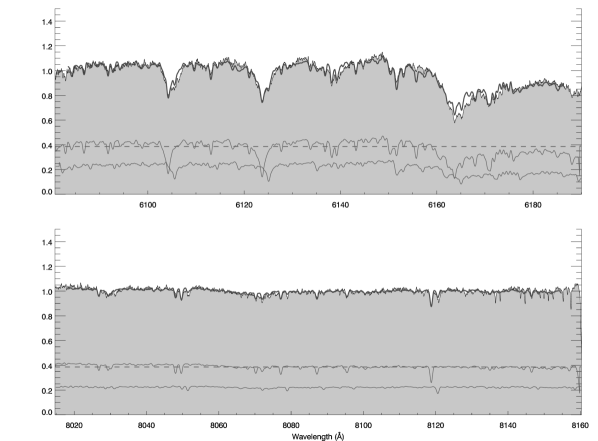
Figure 4: Observed and Model Spectrum of Par 1802. This figure illustrates how the observed spectrum of Par 1802 (black solid line and gray underlying area) can be reproduced by a simple three-component model (thick gray line). This model consists of: an $\sim$M1V template for the primary (upper spectrum), an $\sim$M3V template for the secondary (lower spectrum), and a third featureless spectrum (dashed line). The components are scaled such that the continuum ratio of the components corresponds to 0.39:0.22:0.39. Each panel corresponds to a different order of the Keck/HIRES spectrum. See §3.2.1 for a more complete description.

We find that there is a featureless continuum present in the spectrum of Par 1802, with a luminosity at 7000Å that is approximately equal to that of the primary eclipsing component. This is illustrated for two of the Keck/HIRES spectral orders in Fig. 4, where we show how the combined spectrum can be reproduced by adding the two eclipsing stellar components and a third featureless component. The double-lined nature of the system is obvious around the narrow absorption lines observed in the redder order shown. The best fitting normalized luminosity ratio of all three components is found to be (primary:secondary:extra continuum) 0.39:0.22:0.39 for the spectral orders shown in Fig. 4, which correspond approximately to the $R_{C}$ and $I_{C}$ passbands. The uncertainty in the normalized luminosity of the third component is 0.15, as determined from the scatter of the measurement from the different spectral orders. Figure 4  shows that one cannot reproduce the strong lines around 6120Å without additional continuum. Furthermore, the gravity-sensitive Ca I lines at 6103 and 6122 Å  present in the upper panel, show a good quantitative agreement in strength and shape, that could not be matched by a different gravity and/or extra continuum. This supports that one really needs the extra continuum to explain the fluxes in Par 1802, and that any gravity difference between the templates and Par 1802 are marginal. In order to further quantify this effect, we explored the effect of gravity on the atomic lines using synthetic spectra by decreasing $\log{g}$ from 4.5 to 3.5, and we find that the line depths for atomic lines increase between 0-10%. This would imply that we are slightly overestimating the contribution of the third body, and the flux ratios would be 0.41:0.22:0.36. Thus, we conclude that the difference in gravity between the templates and the PMS eclipsing components does not affect our ability to measure the extra continuum within the quoted uncertainty.

The analysis above does not assume anything about the nature of the third light source. We only state that an extra featureless component is needed in the high-resolution spectrum, and that this is not an artifact of the reduction process. Given that there is no clear infrared excess in the spectral energy distribution of the system as would be characteristic of a disk (see Paper II and §3.2.3 below), and that the H$\alpha$ emission of several mÅ seen in the eclipsing stellar components is too weak to arise from accretion (Paper I), we conclude that the third spectral component must be related to a source other than the two eclipsing stars.

3.2.2 Analysis of Third Light in the Par 1802 Light Curves

We constrain the level of third light ($L_{3}$) in each passband from the spectral measurements described above, and from the amount of third light needed to simultaneously fit all of the observed light curves. The details of the EB modeling and of the exploration of the parameter correlations are described in §4, as are the uncertainties of the system’s fundamental parameters introduced by the uncertainty in $L_{3}$. Here we specifically discuss $L_{3}$ in the context of providing additional evidence for a third star in Par 1802.

The upper limit of $L_{3}$ allowed by the light curves is obtained by setting the inclination ($i$) of the system to 90°, and fitting for $L_{3}$ as a free parameter in our modeling of the light curves (see §4). This is the upper limit because at $i$=90° the eclipses are intrinsically deepest, and thus the observed shallow eclipses imply the maximum dilution. We find that the maximum level $L_{3}$ allowed by the Par 1802 light curves is one that contributes $\sim$75% to the total luminosity of the system in the $I_{C}$-band.

To further explore the relationship between $L_{3}$ and $i$, we fit $L_{3}$ in all passbands for $i$ between 75° and 90°. We find two trends from this analysis. The first one is that, for any given $i$, the required $L_{3}$ is approximately constant for the $I_{C}$JHK_S light curves. The second trend is that $L_{3}$ has a blue excess, i.e., the $V$-band requires an additional 20% $L_{3}$ contribution to fit the eclipse depths than in the other passbands.

Using the spectroscopic measurements described above, we are able to break the degeneracy between $L_{3}$ and $i$. We take $L_{3}$ in the $I_{C}$-band ($L_{3,I_{C}}$) to be 0.39 (see §3.2.1), i.e., 39% of the system’s total luminosity ($L_{{\rm tot},I_{C}}$). That is, $L_{3,I_{C}}$ = 0.39 $\times$ ($L_{1,I_{C}}$ + $L_{2,I_{C}}$ + $L_{3,I_{C}}$) = 0.39 $L_{{\rm tot},I_{C}}$. Similarly, we take $L_{3}$ = 0.39 L_tot for the JHK_S-bands, since our tests above indicated comparable $L_{3}$ in the $I_{C}$JHK_S light curves. For the $V$-band, which our tests above found requires an additional 20% $L_{3}$ contribution relative to the $I_{C}$JHK_S bands, we therefore ascribe $L_{3,V}$ = 0.59 $L_{{\rm tot},V}$. Even though these $L_{3}$ values have high uncertainties ($\sim$15%), we show below that a variation in $L_{3}$ between 5% and 75% of the system’s luminosity does not greatly affect the final physical parameters of the eclipsing components of Par 1802 (see §4).

3.2.3 Spectral Energy Distribution of Par 1802 

In order to probe further into the properties of the third light source in the system, we have attempted to model the full spectral energy distribution (SED) of the system using NextGen model stellar atmospheres (Hauschildt et al., 1999). The SED data consist of the 12 broadband flux measurements described in Paper II, plus the two bluer WISE channels (Duval et al., 2004) covering from 0.36$\mu$m to 8.0$\mu$m. The WISE database has labeled the two longest WISE channels with the ‘h’ flag which means they are likely “ghosts” due to the very low signal-to-noise in those channels (3.8 and 2.0, respectively). To avoid any confusion, we have excluded the two redder WISE channels in our analysis.

For each of the SED modeling attempts described here, we held fixed the radii of the two eclipsing components, as well as their ratio of $T_{\rm eff}$, at the values determined from the detailed light curve modeling of the system (see §4). Thus the luminosity ratio between the eclipsing pair is held fixed at 1.75 at 7000Å, as determined from our spectral decomposition analysis (§3.2.1). We adopted a $T_{\rm eff}$ for the primary eclipsing component of 3675 K based on the system’s reported M2 spectral type (see §4).

We first attempted to model the SED by adding to the eclipsing components a third stellar photosphere with $T_{\rm eff}$ between 3000 and 6000 K, scaled to contribute 39% of the system’s luminosity in the $I_{C}$-band (see §3.2.2). However, regardless of the $T_{\rm eff}$ chosen for the third component, the $L_{3}$ found from our tests with the light curves (§3.2.2) are not well reproduced by such an SED model. For example, the blue excess (i.e., the additional 20% $L_{3}$ in the $V$-band relative to the $I_{C}$-band; §3.2.2) can be modeled by a third component with $T_{\rm eff}$$>$5000 K. However, such a star then contributes far more third light in JHK_S than observed in the light curves, and moreover, the level of the third component’s contribution decreases with increasing wavelength. It is only for a third stellar component with $T_{\rm eff}$ between 3400 and 3700 K, i.e., with a $T_{\rm eff}$ very similar to the average $T_{\rm eff}$ of the eclipsing components, 3560 K (see §4), that the $L_{3}$ contribution remains constant at 39% across the $I_{C}$JHK_S-bands. However, in this case the $L_{3}$ is also $\sim$39% in the $V$-band, i.e., the observed blue excess is not reproduced. Evidently, the source of third light cannot be a simple bare star.

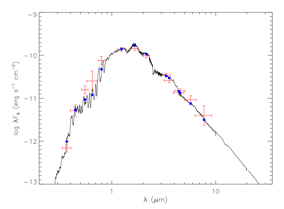
Figure 8: SED fit of Par 1802 including the measured $T_{\rm eff}$ and radii of the eclipsing pair, as well as a third star with $T_{\rm eff}$ and luminosity equal to the primary eclipsing star. The third star also includes a hot spot with $T$=7500 K covering 0.1% of the star’s surface. The free parameters of the fit are $A_{V}$ and distance, for which we derive 1.2$\pm$0.6 and 440$\pm$45 pc, respectively. The reduced $\chi^{2}$ of the fit is 1.94. See §3.2.3 for details.

Finally, we again performed an SED fit in which we included a third stellar component, this time fixing its temperature to the average $T_{\rm eff}$ of the primary and secondary eclipsing components, and once again scaling its luminosity so that it contributes 39% of the total system flux at $I_{C}$-band. We also included a fourth component with a fixed $T_{\rm eff}$ of 7500 K in order to simulate a “hot spot” as observed in many classical T Tauri stars (e.g., Whitney et al., 2003). The luminosity of this fourth component was scaled so that it contributes 20% of the total flux at $V$-band (§3.2.2). The remaining free parameters of the fit are the distance to the system and the line-of-sight extinction to the system. The resulting best fit ($\chi^{2}_{\nu}=$ 1.94; Fig. 8) has a distance of 440$\pm$45 pc and an extinction $A_{V}=$ 1.2$\pm$0.6. These values are in good agreement with the accepted distance to the ONC (436$\pm$20 pc; O’Dell & Henney, 2008) and the typical extinction measured to ONC members (Hillenbrand, 1997).

We have not done a more extensive fitting of possible system parameters, such as different possible temperatures or filling factors for the modeled hot component. Rather, we present this SED as a plausibility check on the inferred levels of third light measured spectroscopically and from the light curves, and to confirm that a putative third star with hot spot does not violate the available SED observational constraints. In Paper II we performed a similar SED fit but including only the two eclipsing stellar components. The fit was acceptable, though a modest excess in the infrared portion of the SED was apparent. The new fit presented here fits the observed fluxes very well over the entire range 0.36–8 $\mu$m.

3.2.4 Summary: The Third Stellar Component in Par 1802

We find clear observational evidence for the existence of a third stellar component in the Par 1802 system. The principal evidence is three-fold. First, there is a clear modulation of the $VI_{C}$JHK_S light curves on a very short period of 0.7355 d. This periodicity manifests itself strongly in the periodogram analysis of the light curves at all observed epochs spanning more than 15 yr (§3.1). Based on the measured radii and $v\sin i$ of the eclipsing components, we can definitively rule out that this period is due to the rotation of either of the two eclipsing stars. Second, a spectral disentangling analysis applied to our high-resolution spectrum of Par 1802 clearly shows the presence of added continuum which dilutes the spectra of the two eclipsing stars (§3.2.1). Third, our simultaneous modeling of the $VI_{C}$JHK_S light curves of Par 1802 clearly shows third light that dilutes the eclipse depths (§3.2.2, and see also §4). The eclipse-depth analysis also clearly indicates that, in the $I_{C}$ and JHK_S passbands, the third light source is characterized by colors very similar to those of the eclipsing stars, but that in $V$ the third source exhibits an additional strong “blue excess” similar to what is observed in Classical T Tauri stars. In addition to these principal lines of evidence, we have shown that the SED of Par 1802 is consistent with a simple SED model comprising the two eclipsing stars and a third star which also includes a blue “hot spot” (§3.2.3). A third stellar component in Par 1802 was also suggested in Paper I by a long-term trend identified in the residuals of the orbit solution, suggesting a low-mass body in a wide, eccentric orbit.

Since the ONC is in front of a very dense, optically-thick cloud, the source of third light cannot be a background object and is likely to be associated with the young cluster. The observed short-period, low-amplitude variability can only arise from a rapidly rotating star and cannot be attributed to either of the eclipsing components because there is no evidence for such rapid rotation in their spectra. The rapid rotation itself suggests a young star. An active late-type star, that is contributing 40% of the system’s luminosity and is rotating with a 0.7355-d period can cause the observed spot modulation ($\sim$3% in the $I_{C}$-band) if its intrinsic variability is $\sim$5%, which is within the typical observed variability for PMS stars. Other other low-mass stars in the ONC have been found to have similarly fast rotation periods (e.g., Stassun et al., 1999). Moreover, if this third star is rapidly rotating and contains a strong contribution from a hot spot as our data suggest, this could very well produce very shallow line profiles that are not detectable in our spectrum and may appear as the measured additional continuum (see §3.2.1 and Fig. 4). As discussed in §3.2.3, including a third star with properties typical of Classical T Tauri stars allows the broadband SED of Par 1802 to be well fit, with a distance and extinction that are consistent with the ONC.

If the third body is indeed actively accreting as suggested by the blue excess, then it must be at a large enough separation from the eclipsing pair to permit it to harbor an accretion disk. At the distance of the ONC, the third star could be separated by as much as $\sim$400 AU and remain spatially unresolved in the $\sim$1 arcsec imaging of our photometric observations.

4 Results: Orbital and Physical Parameters of the Eclipsing Binary Stars in Par 1802 

We use the Wilson-Devinney (WD) based code PHOEBE (Prša & Zwitter, 2005) to do the simultaneous modeling of the EB’s radial velocity (RV) and light curves (LCs). The individual RV and LC datasets are weighted inversely by the square of their r.m.s. relative to the model, and the weights are updated with each fit iteration until convergence.

In all of our fits, we adopt the orbital period $P_{\rm orb}$ determined in §3.1. The rotational synchronicity parameters are calculated from the rotation period of the eclipsing components determined in §3.1, $F_{1}=F_{2}=P_{\rm orb}/P_{\rm rot}$ = 1.0097$\pm$0.0013. We also adopt $T_{\rm eff,1}$=3675$\pm$150 K for the primary star by assuming a primary-to-secondary luminosity ratio of 1.75 (see §3.2.1) and adopting a combined $T_{\rm eff}$$=3560$ K (Luhman, 1999) from Par 1802’s combined spectral type of M2 (Hillenbrand, 1997). The presence of the third star in the system does not significantly affect this average spectral type since its $T_{\rm eff}$ is evidently similar to that of the eclipsing pair (see §3.2). The uncertainty in $T_{\rm eff}$_,1 is dominated by the systematic uncertainty in the spectral-type–$T_{\rm eff}$ scale for low-mass PMS stars.

4.1 Model Fits to Radial-Velocity and Light-Curve Data

To minimize the effect of systematic correlations in the fit parameters, we begin our analysis by doing an initial fit to only the RV curves from Paper II, comprised of 11 measurements for the primary and 9 for the secondary. We initially set $i$=90°, because the RV data provide information only about $\sin{i}$, while $i$ is derived from the light curves later on. We utilize as our initial guesses for the RV solution the best-fit values from Paper II (see Table 1 in that paper) of the parameters to be refined: the semi-major axis ($a\sin i$), the mass ratio ($q\equiv M_{2}/M_{1}$), the systemic velocity ($v_{\gamma}$), and the total system mass $M\sin^{3}i$. The eccentricity ($e$) and the argument of periastron ($\omega$) are later determined through the fit to the RV+LC data. These parameters and their formal uncertainties, derived conservatively from the covariance matrix of the fit to the RV curves alone, are given in Table 10 and are marked with a dagger (^†). The resulting $a\sin{i}$, $M\sin^{3}{i}$, $q$, and $v_{\gamma}$ remain fixed throughout the rest of our analysis.

We next proceed to fit the parameters that depend exclusively on the LC data: $i$, $T_{\rm eff,2}$ (via the $T_{\rm eff}$ ratio), the surface potentials $\Omega_{j}$, and the luminosities, without minimizing for the other parameters. For this task, we include the previously published $I_{C}$ light curve and the $VI_{C}$JHK_S light curves presented in this paper (§2.1). Given that the short period, low-amplitude variability is not attributed to the eclipsing components but to a third body in the system, the light curves are first rectified by removing the sinusoidal variability due to the 0.7355-d period. We do not remove the sinusoidal varation attributed to the rotation of the eclipsing components, as this information is encoded in the model via the $F_{1}$ and $F_{2}$ parameters (see above).

Adopting the third light levels, $L_{3}$, described in §3.2.2, we are able to fit the observed eclipse depths in all bands to our EB model. The effects of the uncertainty in $L_{3}$ on the binary’s physical properties is minimal and is explored in detail below. By fitting the RV and LC data simultaneously (RV+LC), we are able to refine $e$ and $\omega$. We iterate both the LC and RV+LC solutions, until we reach a consistent set of parameters for which the reduced $\chi^{2}$ of the fit is close to $\chi^{2}_{\nu}=1$.

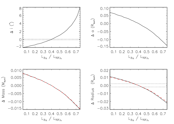
Figure 9: Effects of the $I_{C}$ Third Light on the System’s Parameters. By exploring the effects of the amount of third light on the inclination, we are able to determine that the system’s parameters, in particular those that depend directly on $i$ (semi-major axis, radii and masses), do not change significantly with a change in third light. A variation of the level of third light in the $I_{C}$-band, between 5 and 75% of the total luminosity of the system, corresponds to a change in inclination angle between $\sim$78 and 88°as shown in the top-left panel. The formal errors for the inclination and the radii ($\pm 1\sigma$) are denoted by the horizontal dotted lines in their respective panel; the formal uncertainties for the semi-major axis and the mass are larger than the effect of the variation of the third light on these parameters. This variation of the third light, and consequently of $i$, corresponds to a change in the semi-major axis is of less than $\pm$ 1.5% (top-right panel). It also translates into a change of less than $\pm$ 4% in the masses, corresponding to less than $\pm$ 0.015 M_☉ (bottom-left panel). The solid line and dashed line represent the change in the primary and secondary masses, respectively. The change in the radii of the primary and secondary components of +0.01 and –0.02 R_☉ is presented in the bottom-right panel by the solid line and dashed line, respectively. Thus, the main source of uncertainty in the determination of the inclination and the radii is the uncertainty in the level of third light.

Fig. 1 presents the observed light curves with this best-fit model overplotted, and the physical and orbital parameters of Par 1802 from this model are summarized in Table 10. The results from this study are generally consistent with those from Paper II to within $\sim$1 $\sigma$ (see Table 10). However, the system parameters are now determined more precisely, especially the eccentricity which is important for modeling the tidal evolution history of the system. The system inclination angle is now formally more uncertain than in Paper II, but this is the result of now properly including the effects of the third light levels. However, the third light levels do not strongly affect the physical parameters (e.g., Fig. 9). The reported parameter uncertainties of our best solution include both the formal and heuristic parameter uncertainties (obtained from a direct $\chi^{2}$ mapping of the parameter space), as well as the uncertainties associated with our choice of third light levels, as we now discuss.

4.2 Effects of Third Light

$L_{3}$ and $i$ are highly degenerate, i.e., an increase in $i$ may be compensated by an increase in $L_{3}$, rendering the same goodness of the fit. Consequently, $L_{3}$ most strongly impacts the parameters that depend directly on $i$: $a$, the radii, and the masses. The $T_{\rm eff}$ ratio is weakly dependent on a change in $i$ and its corresponding $L_{3}$, because the $T_{\rm eff}$ ratio is constrained by the observed relative depths of the eclipses which is itself not strongly dependent on $i$.

To explore these degeneracies as a function of $L_{3}$, we vary $L_{3}$ in the $I_{C}$-band such that it contributes between 5% and 75% of the system’s total luminosity, adjusting $L_{3}$ in the other bands according to the trends identified in §3.2.2. Fig. 9 shows the relationship between the change in $L_{3}$ and $i$, $a$, and the measured masses and radii of the eclipsing components. We find that the corresponding value for $i$ for this variation in $L_{3}$ lies in the range 78–88°. Since this change in $i$ is greater than its formal error of $\sim$0.1°, we adopt $\sigma_{i}=^{+8.0}_{-2.0}$ degrees. The change in the value of $a$ as $L_{3}$ is varied is less than 2%. Thus, the masses vary by less than 4% or 0.015 $M_{\sun}$. These changes are well below our formal uncertainty of 0.032 $M_{\sun}$, which includes the above uncertainty in $i$. The radii change by ${}^{+0.01}_{-0.02}$ $R_{\sun}$, or $\pm$1%. Without including the uncertainty in $L_{3}$, the formal errors from the RV+LC fit are 0.002 $R_{\sun}$, for both the primary and secondary. The main source of uncertainty in the determination of the radii is therefore the uncertainty in $L_{3}$. Therefore we adopt conservatively a 1-$\sigma$ error of 0.02 $R_{\sun}$ for the radii of both eclipsing components.

4.3 Non-Zero Orbital Eccentricity

Interestingly, our best-fit solution yields an orbital eccentricity that is significantly different from zero: $e=0.0166^{+0.0017}_{-0.0026}$. Small eccentricities can arise spuriously because of the positive-definite nature of $e$. Thus it was of concern that the best-fit argument of periastron is very close to $\frac{3\pi}{2}$. Moreover, $e$ and $\omega$ are correlated parameters through $e\cos\omega$ and $e\sin\omega$. Therefore we have explored $e$ and $\omega$ in depth using two approaches.

First, we estimated $e$ and $\omega$ from simple arguments involving the phases of primary and secondary eclipse minima, $t_{p}$ and $t_{s}$, and from the phase duration of each eclipse, $\Theta_{p}$ and $\Theta_{s}$. The derived $e$ and $\omega$ are then related as follows (Kallrath & Milone, 2009): $e\cos{\omega}\approx\pi(t_{s}-t_{p}-\frac{1}{2})/(1+\csc^{2}{i})$ and $e\sin{\omega}\approx(\Theta_{p}-\Theta_{s})/(\Theta_{p}+\Theta_{s})$. A lower limit for $e$ may thus be estimated by assuming $|\cos{\omega}|=1$. In order to measure the separation and duration of the eclipses, we fit a Gaussian to both minima in the phased $I_{C}$-band and obtain from the phases at which they occur that their separation is $t_{s}-t_{p}=0.49799\pm 0.00025$, where the uncertainty is from the formal uncertainty on the centroids of the fitted Gaussians. Note that by fitting the eclipses in the entire phased light curve we are effectively averaging over the random scatter in the individual eclipse times (see Section 3.1). The phase separation of the eclipses differs from 0.5 by 8-$\sigma$. Hence, we can set as a firm lower limit, $e\geq 0.0031$. The separation of the minima in conjunction with the measured durations, $\Theta_{p}$ = 0.1010$\pm$0.0007 and $\Theta_{s}$ = 0.0877$\pm$0.0012, render $\omega\approx 1.514\pm 0.004$ $\pi$ radians. These $e$ and $\omega$ are estimates only, but demostrate that $e>$ 0 from simple theoretical arguments unrelated to light curve modeling.

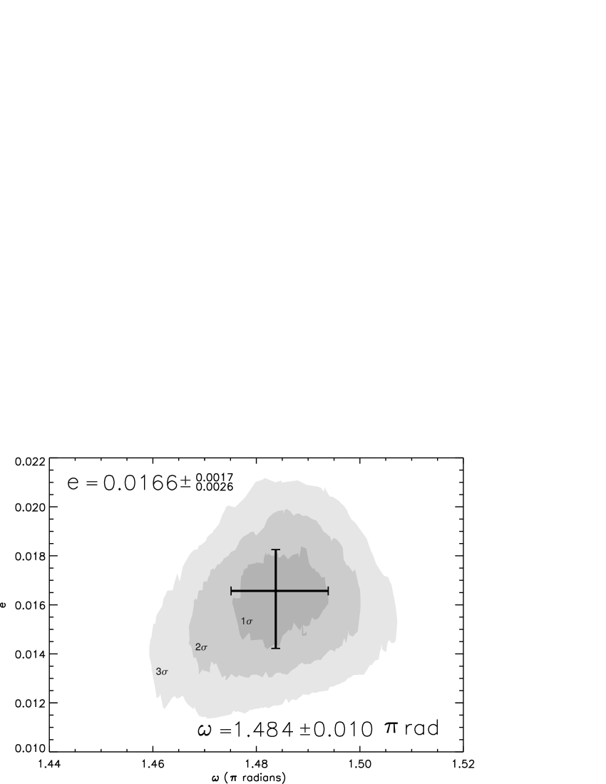
Figure 5: RV+LC Joint Confidence Levels for $e-\omega$. Given our dataset, we are able to measure the very small but significant orbital eccentricity of the EB. The heuristic errors of the eccentricity $e$ and the argument of periastron $\omega$ are estimated by the variation of a $\chi^{2}$-distribution with two degrees of freedom with $e$ and $\omega$. The center of the cross marks the point at which the $\chi^{2}$ of the RV+LC fit attains its minimum value; its length and width indicate the 1-$\sigma$ uncertainties for the sampled parameters as given by the innermost contour level. Each subsequent contour represents a 1-$\sigma$ increase. The RV+LC parameter hyperspace is sampled for 0.0 $<\omega<$ 2$\pi$ and 0.0 $<e<$ 0.1; this is the same parameter range sampled for the LC contours shown in Fig. 6.

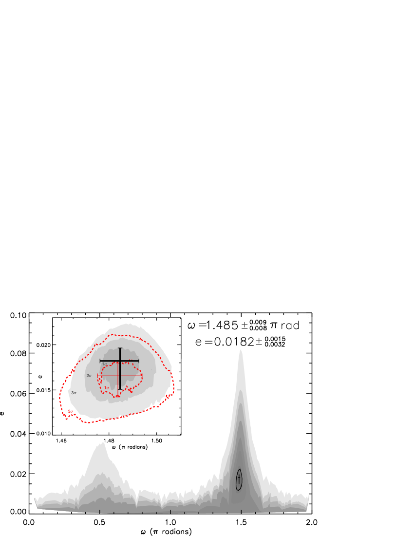
Figure 6: LC Joint Confidence Levels for $e-\omega$. The LC confidence contours allows us to confirm that the values for $e$ and $\omega$ from the RV+LC contours are not systematically skewed by the weighting of the data, due to the abundant number of photometric data in comparison to the number of RV measurements. The figure shows the sampled parameter cross section in its entirety. The cross marks the lowest-$\chi^{2}$ point to the LC fit with 1-$\sigma$ uncertainties, surrounded by the solid line 3-$\sigma$ confidence level. The shaded contours beyond 3-$\sigma$ do not correspond to a particular uncertainty level but are shown to display the two valleys in $\chi^{2}$ when the orbit’s semi-major axis is parallel to the line-of-sight. The inset shows in detail the confidence interval for $e$ and $\omega$ within 3-$\sigma$; and for comparison, the dashed lines denote the 1 and 3-$\sigma$ RV+LC contours from Fig. 5.

Second, we performed a detailed sampling of the parameter cross-section between $e$ and $\omega$ by fitting all of the RV and light curve data in order to determine the best-fit values of these parameters and their heuristic uncertainties from a detailed examination of the shape of the $\chi^{2}$ space. Fig. 5 shows the joint confidence levels for $e$ and $\omega$ following the variation of a $\chi^{2}$-distribution with two degrees of freedom around the RV+LC solution’s minimum. This cross section was sampled 1750 times by randomly selecting values for $e$ in the range 0.0–0.1, and for $\omega$ in the range 0–2$\pi$ radians. The phase shift, which gives the orbital phase at which the primary eclipse occurs, is strongly correlated with both explored parameters and is therefore minimized for each set of randomly selected values; whereas the rest of the parameters are less correlated and kept constant at their best-fit values. In order to verify that $e$, $\omega$, and their uncertainties are not artificially skewed by the weighting of both the RV and light curves as undertaken in PHOEBE by WD, given that our data set is comprised mostly of photometric measurements, we sampled the same range in $e$ and $\omega$ 1900 times by fitting to the light curves alone and obtaining their LC confidence contour levels. We find that the LC contours, shown in Fig. 6, are very similar to the RV+LC contours (Fig. 5). The minimum value of $\chi^{2}$ to the RV+LC fit is $e$ = 0.0166${}_{-0.0026}^{+0.0017}$ and $\omega$ = 1.484$\pm$0.010 $\pi$ radians. For the LC fit, it is $e$ = 0.0182${}_{-0.0032}^{+0.0015}$ and $\omega$ = 1.485${}_{-0.008}^{+0.009}$ $\pi$ radians. The detailed LC contours up to 3-$\sigma$ are shown in the inset in Fig. 6; for comparison, the 1-$\sigma$ and 3-$\sigma$ RV+LC contours are overplotted in the dashed lines. The two sets of contours are consistent with one another, and thus we adopt the values of $e$ and $\omega$ and their heuristic uncertainties from the RV+LC contours.

Extensive numerical integrations, like those performed for the system $\upsilon$ Andromedae (Barnes et al., 2011), spanning the plausible range of orbits and masses of a third body that produce the measured eclipse timing variations (see §3.1) and small eccentricity are beyond the scope of this paper, but could be the best way to constrain the mass and orbit of an unseen companion.

4.4 Temperature Ratio and Stellar radii

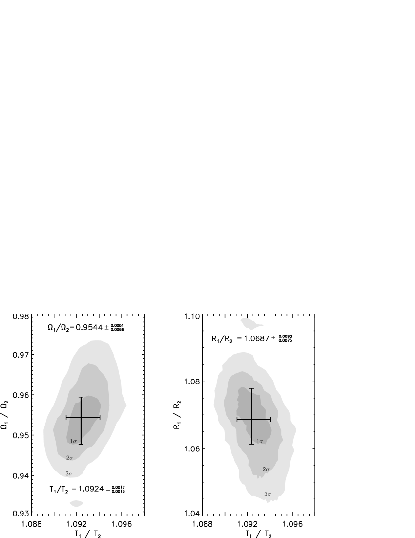
Figure 7: Joint Confidence Levels for ($T_{\rm eff,1}/T_{\rm eff,2}$) – ($R_{1}/R_{2}$). Similar to Fig. 5 and Fig. 6, the significance levels given by the contours are representative of the change in $\chi^{2}$ as the ratios of temperatures and radii are explored. Even though the masses of the components are almost equal, $q$ = 0.985 $\pm$ 0.029, the effective temperatures differ by 9.2$\pm$0.2%, and the radii of the eclipsing binary components by 6.9$\pm$0.8%. Consequently, their luminosities differ by 62$\pm$3%.

We sampled the parameter hyperspace between ($T_{\rm eff,1}/T_{\rm eff,2}$) and ($R_{1}/R_{2}$) over 2000 times, shown in Fig. 7, in order to confirm the significance of the differences in radii and $T_{\rm eff}$ between the eclipsing components of Par 1802. We explore the $T_{\rm eff}$ ratio in the range 1.0382–1.1271. The radius for the component of a detached EB depends on the surface potentials as $\sim$$1/\Omega_{j}$; so the ratio of the radii was sampled by choosing values for $\Omega_{1}$ in the range 5.5–8.4, and minimizing for $\Omega_{2}$. To facilitate the convergence of $\Omega_{2}$, we exploit the fact that the sum of the radii must remain the same due to the observational constraint provided by the eclipse durations. We confirm that the ratio of $T_{\rm eff}$ as shown in Paper II is different from unity, $T_{\rm eff,1}/T_{\rm eff,2}$ = 1.0924${}^{+0.0017}_{-0.0013}$. We also confirm this disparity in the case of the ratio of the eclipsing components radii, $R_{1}/R_{2}$ = 1.0687${}^{+0.0093}_{-0.0075}$.

5 Discussion: Possible Origins of the ‘Dissimilar Identical Twins’ in Par 1802 

Par 1802 is a unique system providing important observational constraints in the low-mass regime at the earliest evolutionary stages. Not only does it provide precise and direct measurements of the mass and the radius of each of its components; but because the component masses are very nearly equal ($q=0.985\pm 0.029$, Table 10), Par 1802 affords a unique opportunity to examine the degree to which two otherwise identical stars in a close binary share identical evolutionary histories. Despite having equal masses, the stars’ radii that we have measured accurately to $\sim$1%, differ by 7%. The measured $T_{\rm eff}$ ratio, accurate to $\sim$0.2%, indicates that the individual stellar $T_{\rm eff}$ differ by 9%.

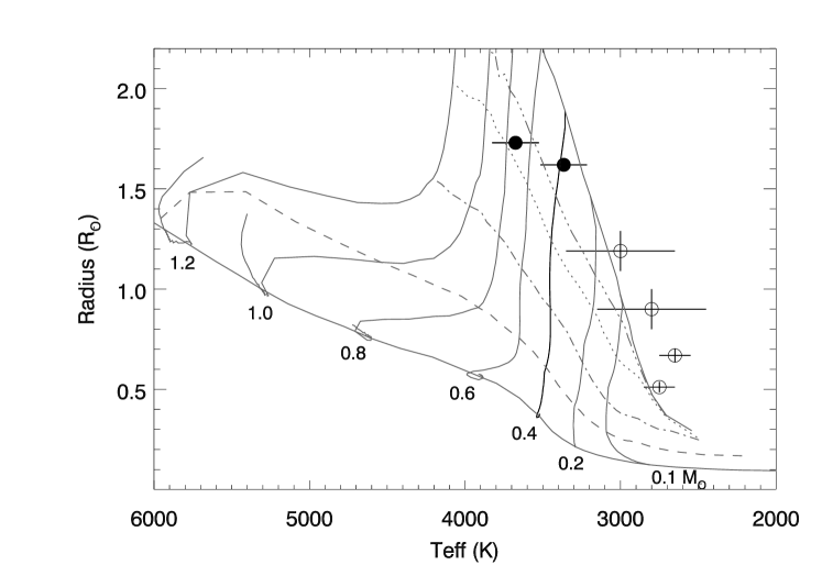
Figure 11: $T_{\rm eff}$–Radius Diagram. The observed EB properties and the BCAH98 theoretical isochrones (from 1 Myr to 1 Gyr) are denoted as described in Fig. 10. The lines that start at the 1 Myr isochrone (i.e., the solid line at far-right top corner) and descend almost vertically during the first few Myr represent the evolution of stars of different masses (from 0.1 to 1.2 M_☉) as predicted by BCAH98. In this diagram, it is clear that the components of Par 1802 are young; however, the measured $T_{\rm eff}$ and radii of both eclipsing components cannot be described by the 0.4 M_☉ mass track. It is only the secondary $T_{\rm eff}$ that is consistent with the measured mass. Additional heating mechanisms that might explain the observed primary $T_{\rm eff}$ are explored in §5.

In this section, we consider possible implications of these physical differences between the two eclipsing stars in Par 1802. We compare the measured properties of Par 1802 to four different pre-main sequence stellar evolutionary models: DAM97 (D’Antona & Mazzitelli, 1997); SDF00 (Siess et al., 2000); BCAH98 (Baraffe et al., 1998), and PS99 (Palla & Stahler, 1999). As an example, in Fig. 10, we show the predicted masses and radii of stars from $0.01-0.6$ M_⊙ and with a range of ages from 1 Myr to 1 Gyr from the BCAH98 evolutionary models compared to the observed properties of Par 1802. In Figs. 10–11, the physical properties of the two other known PMS EBs in the ONC with the lowest masses and the youngest ages (2M0535$-$05, and JW 380) are shown to provide context. We show these particular models because they are specifically designed to predict the properties of very low mass objects (late-type stars and brown dwarfs) at very young ages ($\tau\geq 1$ Myr), and they are reasonably successful at reproducing the structural properties of these particular systems.

Despite the complex phenomena that young objects can potentially experience in their very early evolution (i.e., accretion, magnetic activity, contraction, rapid rotation, tidal interactions, etc.), the observed radii of these objects are surprisingly well predicted by theoretical isochrones with an age consistent with the ONC (1–2 Myr). The radii of the equal-mass eclipsing components of Par 1802 are enlarged, as expected for pre-main sequence stars. However, when we look in more in detail, the measured radii of the two eclipsing components are significantly different, and this is not predicted by a single theoretical isochrone. Moreover, the effective temperatures of these two stars are also significantly different. In the temperature-radius diagram that compares the BCAH98 models with the observed properties from the PMS EBs (Fig. 11), this implies that the two equal-mass stars cannot both be fit by the same mass track.

In the first 10 Myr, as these low mass stars descend along the Hyashi track to the main sequence, a rapid contraction in radius at roughly constant temperature is predicted. All the models we examined show similar trends from 1–10 Myr, however the BCAH98 models predict a cooler temperature for this contraction by $\sim$200 K than the other three models. Furthermore, the DAM97 model is unique in that it shows an additional rapid evolution in $T_{\rm eff}$ prior to the first 1 Myr (as shown in Paper II). Despite some genuine successes, no existing single star evolutionary model (that does not include accretion, magnetic activity, tidal heating, rotation, detailed convection) is able to reproduce the observed properties of both eclipsing components of Par 1802 with a single age and mass.

Moreover, the different predictions by each of the theoretical models lead to different possible physical interpretations for Par 1802. The $T_{\rm eff}$ and radius of the secondary star is well reproduced by the BCAH98 models for a 0.4 M_⊙ star with an age of  1–2 Myr (see Fig. 11), but the primary star is too hot for its mass. However, the models by DAM97, PS99, and SDF00 predict a 2 Myr, 0.4 M_⊙ star to have a $T_{\rm eff}$ consistent with the primary star, but overestimate the temperature of the secondary. This comparison suggests that one of the two components (probably the primary star) may have experienced some form of additional heating making it unexpectedly hotter than its twin. In addition, as discussed in Paper II, the DMA97 models suggest a small age difference could be invoked to explain the differences in physical properties between the two eclipsing components of Par 1802 if the system is hotter by $\sim$250 K and younger than 1 Myr (see §5.2). We consider the possible explanations below in more detail.

5.1 Magnetic Activity

Evolutionary models have typically not included the effects of magnetic fields because of the complexity and difficulty involved in their modeling. However, the effects of magnetic fields are thought to be the cause of the enlarged radii and cool temperatures of field M dwarfs found in eclipsing binary systems (López-Morales, 2007). The presence of spots and/or the reduction of the convective efficiency of the star, due to increased magnetic activity, lower the effective temperature and increase the radius in order to maintain the star’s luminosity (Chabrier et al., 2007). Par 1802’s nearly equal-mass components should have similar convection zone depths and are rotating at similar rates, thus it is likely that they have similar magnetic activity levels. Moreover, the measured H$\alpha$ emission of both stars is weak. If magnetic activity were the cause of the discrepant radii and effective temperatures in Par 1802, we would expect the cooler component to have the larger radius. However, we find the opposite. The secondary star has the smaller radius and cooler temperature, thus magnetic activity is unlikely to be causing the disparate radii and temperature reversal found between the twin components of Par 1802.

5.2 Competitive Accretion

As discussed in Paper II, a difference in age of a few $\times 10^{5}$ yr could potentially explain the observed differences in $T_{\rm eff}$ and radius for the eclipsing stars in Par 1802. The idea here is that mass equalizing mechanisms during the binary formation process may have preferentially directed accretion from the circumbinary disk to the (initially) lower-mass component, leading that star to cease the phase of heavy accretion later than its companion, and causing its “birth” to be effectively delayed relative to its companion (i.e., causing it to appear younger). This “competitive accretion” scenario has been specifically advanced in the context of Par 1802 by Simon & Obbie (2009).

If the $T_{\rm eff}$’s for both stars could be shifted $\sim$250 K hotter (while preserving the accurately measured $T_{\rm eff}$ ratio), implying a $\sim$2$\sigma$ shift relative to the likely systematic uncertainty on the absolute $T_{\rm eff}$ scale for these stars, the stars are best matched by the DAM97 models, which predict that a 0.4 M_☉ star decreases in $T_{\rm eff}$ during the first Myr. This would imply that the primary star is the younger component, being both hotter and larger. In this scenario, the primary will presumably evolve along the 0.4 M_☉ track and, within a few Myr, appear identical to its (presumed slightly older) twin.

5.3 Tidal Evolution and Heating

Another potential explanation for the observed differences in luminosity of the Par 1802 EB components is the presence of additional energy sources. We have determined that the orbit of Par 1802 is not circular, but rather has a non-zero eccentricity of $e$=0.0166$\pm$0.003. In addition, we have measured the rotation period of the EB components to be very close to but significantly different than the orbital period (§3.1). Consequently, the EB components should be experiencing some degree of tidal interaction. In this section, we consider the role of tides and the amount of tidal heating that the two stars may have experienced during their lifetimes in order to reproduce their observed physical properties. In particular, we wish to determine whether the primary star could have acquired enough additional tidal heating to explain its apparent over-luminosity relative to its twin.

A substantial body of research is devoted to tidal theory. The reader is referred to Hut (1981), Ferraz-Mello et al. (2008), Leconte et al. (2010), Mazeh (2008), Zahn (2008) and references therein for a more complete description of the derivations and nuances of various theoretical treatments. For this investigation, we consider the so-called “constant phase lag” (CPL) and “constant time lag” (CTL) models, the details of which are provided in Appendix B (and see Heller et al., 2011). Our approach is not intended to be a definitive treatment of the tidal evolution of this binary. Rather we estimate tidal effects using standard assumptions and linear theory. More detailed modeling could prove enlightening, but is beyond the scope of this investigation. Even so, the discussion below indicates that standard assumptions suggest tidal heating is important in this binary.

The CPL and CTL models assume that the physical properties of the stars are constant with time. However, as the Par 1802 system is very young ($\sim$1 Myr), the radii are expected to be contracting quickly. This contraction could have a profound effect on tidal processes as the radius enters both the CPL and the CTL models at the fifth power (see Eqs. B5 and B14). Radial contraction will also enter into the angular momentum evolution through the rotational frequency (Eqs. B3 and B12). Thus we have added radial contraction to the CPL and CTL models, in a manner similar to that in Khaliullin & Khaliullina (2011), but note that their treatment does not include obliquity effects. D’Antona & Mazzitelli (1997) and Baraffe et al. (1998) provide from their calculations the time rate of change of the radius, $dR/dt$ in R_⊙/Myr, for 0.4 M_⊙ stars. We fit their models with a third order polynomial using Levenberg-Marquardt minimization,

$$\frac{dR}{dt}=a_{0}+a_{1}t+a_{2}t^{2}+a_{3}t^{3},$$ (1)

where $a_{0}...a_{3}$ are constants listed in Table 11. For simplicity, we assume the radial contraction is independent of the tidal evolution. Therefore, the “radius of gyration” $r_{g}$, i.e., the moment of inertia is $M(r_{g}R)^{2}$, is held constant, and moreover, we can express the change in stellar spin due solely to radial contraction as

$$\frac{d\omega}{dt}=-\frac{2\omega}{R}\frac{dR}{dt}.$$ (2)

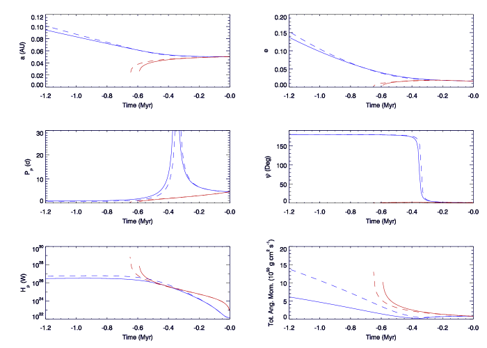
Figure 12: History of the eclipsing components of Par 1802 due to tidal processes and radial contraction for $\psi_{P}=1^{\circ}$ and $\psi_{S}=0$. Blue curves are for the CTL model, and red the CPL. Solid curves use the Baraffe et al. (1998) radial contraction model, dashed the D’Antona & Mazzitelli (1997) model. Top Left: Semi-major axis. Top Right: Orbital eccentricity. Middle Left: Primary’s rotation period. Middle Right: Primary’s obliquity. Bottom Left: Primary’s tidal heat. Bottom Right: The total angular momentum of the system.

In Fig. 12, we present the history of Par 1802 due to both tidal evolution (for both the CPL and CTL models) and radial contraction (for both the DM97 and BCAH98 stellar evolution models). The behavior of the resulting tidal evolution history is qualitatively different as compared to the evolution without radial contraction effects (see Appendix B). We assume the primary star’s obliquity $\psi_{P}$ = 1° at the present time, i.e., $t=0$, in order to be able to determine the evolution of $\psi_{P}$. The CTL model evolution (blue curves) predicts that the stellar obliquities were anti-parallel up to 0.5 Myr ago, and then $\psi_{P}$ rapidly “flipped” (actually its rotation was halted and then reversed). For the CPL model (red curves), the evolution breaks down at $\sim$0.5 Myr in the past as the stars are predicted to have been merged (and consequently the model fails to conserve angular momentum within a factor of 10; bottom right panel). In principle this could be taken as a constraint on the system’s maximum age, but more likely this reflects the limitations of the simplified linear tidal theory that we have adopted; the model is unable to account for effects such as Roche lobe overflow that would certainly have been important if the stars had once been in physical contact. This behavior of the CPL model could be avoided by tuning the model’s $Q$ parameter (here we have adopted the standard value for pre-main sequence stars of $10^{6}$ (see Zahn, 2008)), however for the current discussion we discard the prediction of formerly merged stars and instead adopt the CTL model predictions as more physically plausible.

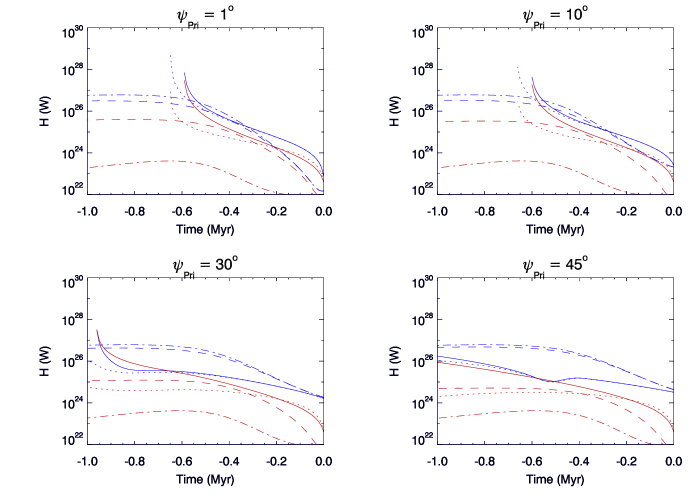
Figure 13: Comparison of heating histories of the two eclipsing components of Par 1802. The primary is represented by blue curves, secondary by red. In all cases the obliquity of the secondary is zero. Solid curves assumed the CPL and Baraffe et al. (1998) models, dotted CPL and D’Antona & Mazzitelli (1997) models, dashed CTL and Baraffe et al. (1998), and the dash-dotted the CTL and D’Antona & Mazzitelli (1997) models. From top left to bottom right

Finally, in Fig. 13 we consider whether tidal effects can explain the increased radius of the primary. We consider a range of possibilities, all of which assume $\psi_{S}=0$ for simplicity. There are four possible combinations of models: CTL-B98, CPL-B98, CTL-DM97, and CPL-DM97. The CPL models (solid and dotted curves) do not predict much difference in the tidal heating rates between the primary and secondary star. The CTL-B98 model (dashed curve) predicts about a factor of 10 difference between the stars, and with the primary receiving $>10^{26}$ W as recently as 0.2 Myr ago ($\psi_{P}=45^{\circ}$). The model that predicts the largest difference in the heating rates between the two stars is the CTL-DM97 case (dot-dashed curves), which predicts a difference in heating of more than 3 orders of magnitude as recently as 0.5 Myr ago. Moreover, the heating rate seems to level out at about $10^{26}$ W (and roughly independent of $\psi_{P}$). However, the CTL models, as shown in Fig. 12, predict that the obliquities were anti-parallel when the heating rates are most different.

A tidal heating rate of $\sim 10^{26}$ W is comparable to the observed difference between the Par 1802 primary and secondary stars’ luminosities ($\Delta L\approx 7\times 10^{25}$ W; see Table 10). The models in Fig. 13 are able to supply at least this amount of tidal heating to the primary up to $\sim$0.2 Myr in the past. Thus, assuming that the primary star will have retained this extra heat for at least 0.2 Myr, we conclude that tidal processes are able to provide a sufficient energy source to explain the differences in the luminosities of the Par 1802 EB pair. However, this requires the spins to have been misaligned, at least in the past. Observation of misaligned spin axes in Par 1802 (e.g., via the Rossiter-McLaughlin effect) would provide strong additional evidence in favor of this interpretation, though it may be a challenging observation if the obliquity is small.

6 Summary

Parenago 1802 is a pre–main-sequence, double-lined, detached eclipsing binary, and is the youngest known example of a low-mass system with a mass ratio of unity ($q$=0.99$\pm$0.03). It presents a unique source of observational constraints for low-mass stars during the early stages of their evolution. Contrary to what theoretical evolutionary models predict for stars of the same mass, composition and age, the radii of the eclipsing pair differ by 6.9$\pm$0.8%, their effective temperatures differ by 9.2$\pm$0.2%, and consequently their luminosities differ by 62$\pm$3%, despite their masses being equal to within 3%.

The Par 1802 system appears to include an unresolved, low-mass third star that is rapidly rotating and likely accreting (i.e., a Classical T Tauri star) in a wide orbit about the eclipsing pair. This third star manifests itself in multiple ways, including a very short period modulation of the light curves, excess continuum in the spectra, and dilution of the eclipse depths in the light curves. The broadband spectral energy distribution of the Par 1802 system can be modeled by two stars with the measured properties of the eclipsing pair, plus a third low-mass star including an accretion hot spot, at a distance of 440$\pm$45 pc, consistent with the distance to the Orion Nebula Cluster.

We measure the rotation period of the eclipsing stars and find that they are rotating with a period that is slightly but significantly faster than the orbital period. Moreover, the orbit has not yet circularized, presenting a small but significant eccentricity, $e$=0.0166$\pm$0.003. These orbital and rotational characteristics provide important insight into the tidal interactions at a very young age that lead to the synchronization and circularization of binaries. We show that tidal interactions during the past 1 Myr history of the system could plausibly have injected sufficient heat into one of the eclipsing components to explain its over-luminosity relative to its twin. This explanation predicts that the epoch of high tidal heating terminated $\sim$0.2 Myr ago, and thus requires that the over-luminous component have retained the tidal heat for at least the past 0.2 Myr (assuming a nominal system age of 1 Myr). This explanation also predicts that the eclipsing pair’s rotation axes may yet be misaligned, which could be observable via the Rossiter-McLaughlin effect.

Appendix A Verification of Periodicity Analysis with Synthetic Signals

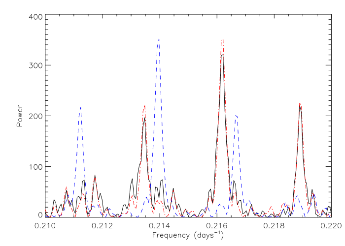
Figure 14: OFE $I_{C}$ and Synthetic Periodograms. We compare the periodogram of the OFE $I_{C}$ light curve (solid line) around the frequency of 1/$P_{1}$ $\simeq$ 0.216 d^-1 with two synthetic sinusoidal signals, one with a period equal to $P_{1}$ (dashed-dotted line) and another with a period of $P_{\rm orb}$ (dashed line). Both synthetic signals have been sampled to the timestamps of the $I_{C}$ data to preserve its statistical characteristics; and their periodograms have been scaled to the amplitude of the OFE $I_{C}$ periodogram. The three-peaked structure around the most significant peak is due to the yearly sampling of the light curve; the side-peaks are separated from the central peak by a frequency of 1/360 d^-1. Since we are able to clearly distinguish between the periodogram peaks of the $P_{1}$ signal and those of the $P_{\rm orb}$ signal, we conclude the $P_{1}$ is significantly distinct from the orbital period.

To ensure that the peak that corresponds to $P_{1}$, identified as the rotation period of the eclipsing components, is significantly different than that of the orbital period given the available dataset, we create two synthetic sinusoidal signals that are sampled using the timestamps of the OFE $I_{C}$ light curve: one with a period equal to $P_{1}$ and another to $P_{\rm orb}$. After running the synthetic signals through the periodicity analysis described in §3.1, we compare their periodograms to that of the OFE $I_{C}$ light curve. Fig. 14 shows that the periodogram of the OFE $I_{C}$ light curve (solid line) around the frequency of 1/$P_{1}$ $\simeq$ 0.216 d^-1 is almost equal to the normalized periodogram of the synthetic signal with the same period (Fig. 14, dash-dotted line), as expected. Moreover, the periodogram of the synthetic signal with a period equal to the orbital period (Fig. 14, dashed line) is clearly distinct from the other two periodograms. By directly assessing the window function of the data through the periodograms of the synthetic periodic signals, we are able to discard the possibility that the three-peaked structure found in the periodograms centered around the most prominent peaks is an artifact of our periodicity analysis. The periodograms of the synthetic signals, as shown in Fig. 14, also present the three-peaked structure confirming that it arises from the sampling of the data and that we have enough frequency resolution to discern $P_{1}$ from $P_{\rm orb}$.

Appendix B Details of Tidal Evolution Models

For our calculations of tidal evolution, we employ “equilibrium tide” models, originally derived by Darwin (1879, 1880). These models assume the gravitational potential of the tide raiser can be expressed as the sum of Legendre polynomials and that the elongated equilibrium shape of the perturbed body is slightly misaligned with respect to the line which connects the two centers of mass. This misalignment is due to dissipative processes within the deformed body, i.e., friction, causing a secular evolution of the orbit as well as the angular momenta of the two bodies. When consistently calculating the tidal interaction of two bodies, the roles of the tide raiser and the perturbed body can be switched. This approach leads to a set of six coupled, non-linear differential equations, but note that the model is in fact linear in the sense that there is no coupling between the surface waves which sum to the equilibrium shape.

B.1 The Constant Phase Lag Model

In the “constant-phase-lag” (CPL) model of tidal evolution, the angle between the line connecting the centers of mass and the tidal bulge is assumed to be constant. This approach has the advantage of being analogous to a damped driven harmonic oscillator, a well-studied system, and is quite commonly utilized in planetary studies (e.g., Goldreich & Soter, 1966). In this case, the evolution is described by the following equations

$$\frac{\mathrm{d}e}{\mathrm{d}t}\ =\ -\frac{ae}{8GM_{1}M_{2}}\sum_{i\,\neq\,j}Z^{\prime}_{i}\Bigg{(}2\varepsilon_{0,i}-\frac{49}{2}\varepsilon_{1,i}+\frac{1}{2}\varepsilon_{2,i}+3\varepsilon_{5,i}\Bigg{)}$$ (B1)

$$\frac{\mathrm{d}a}{\mathrm{d}t}=\frac{a^{2}}{4GM_{1}M_{2}}\sum_{i\,\neq\,j}Z^{\prime}_{i}{\Bigg{(}}4\varepsilon_{0,i}+e^{2}{\Big{[}}-20\varepsilon_{0,i}+\frac{147}{2}\varepsilon_{1,i}+\frac{1}{2}\varepsilon_{2,i}-3\varepsilon_{5,i}{\Big{]}}$$

$$-4\sin^{2}(\psi_{i}){\Big{[}}\varepsilon_{0,i}-\varepsilon_{8,i}{\Big{]}}{\Bigg{)}}$$ (B2)

$$\frac{\mathrm{d}\omega_{i}}{\mathrm{d}t}\ =\ -\frac{Z^{\prime}_{i}}{8M_{i}r_{\mathrm{g},i}^{2}R_{i}^{2}n}{\Bigg{(}}4\varepsilon_{0,i}+e^{2}{\Big{[}}-20\varepsilon_{0,i}+49\varepsilon_{1,i}+\varepsilon_{2,i}{\Big{]}}$$ (B3)

$$+\ 2\sin^{2}(\psi_{i}){\Big{[}}-2\varepsilon_{0,i}+\varepsilon_{8,i}+\varepsilon_{9,i}{\Big{]}}{\Bigg{)}}$$

$$\frac{\mathrm{d}\psi_{i}}{\mathrm{d}t}\ =\ \frac{Z^{\prime}_{i}\sin(\psi_{i})}{4M_{i}r_{\mathrm{g},i}^{2}R_{i}^{2}n\omega_{i}}{\Bigg{(}}{\Big{[}}1-\xi_{i}{\Big{]}}\varepsilon_{0,i}+{\Big{[}}1+\xi_{i}{\Big{]}}{\Big{\{}}\varepsilon_{8,i}-\varepsilon_{9,i}{\Big{\}}}{\Bigg{)}}\ ,$$ (B4)

where $e$ is eccentricity, $t$ is time, $a$ is semi-major axis, $G$ is Newton gravitational constant, $M_{1}$ and $M_{2}$ are the two masses, $R_{1}$ and $R_{2}$ are the two radii, $\omega$ is the rotational frequency, $\psi$ is the obliquity, $r_{g}$ is the “radius of gyration,” i.e., the moment of inertia is $M(r_{g}R)^{2}$, and $n$ is the mean motion. The quantity $Z^{\prime}_{i}$ is

$$Z^{\prime}_{i}\equiv 3G^{2}k_{2}M_{j}^{2}(M_{i}+M_{j})\frac{R_{i}^{5}}{a^{9}}\ \frac{1}{nQ_{i}}\ ,$$ (B5)

where $k_{2}$ is the Love number of order 2, and tidal $Q$ is the “tidal quality factor.” The parameter $\xi_{i}$ is

$$\xi_{i}\equiv\frac{r_{\mathrm{g},i}^{2}R_{i}^{2}\omega_{i}an}{GM_{j}},$$ (B6)

where $i$ and $j$ refer to the two bodies. The signs of the phase lags are

$$\begin{array}[]{l}\varepsilon_{0,i}=\Sigma(2\omega_{i}-2n)\\ \varepsilon_{1,i}=\Sigma(2\omega_{i}-3n)\\ \varepsilon_{2,i}=\Sigma(2\omega_{i}-n)\\ \varepsilon_{5,i}=\Sigma(n)\\ \varepsilon_{8,i}=\Sigma(\omega_{i}-2n)\\ \varepsilon_{9,i}=\Sigma(\omega_{i})\ ,\\ \end{array}$$ (B7)

with $\Sigma(x)$ the sign of any physical quantity $x$, thus $\Sigma(x)~{}=~{}+~{}1~{}\vee~{}-~{}1~{}\vee~{}0$.

The tidal heating of the $i$th body is due to the transformation of rotational and orbital energy into frictional heating. The heating from the orbit is

$$\dot{E}_{\mathrm{orb},i}=\ \frac{Z^{\prime}_{i}}{8}\ \times\ {\Big{(}}\ 4\varepsilon_{0,i}+e^{2}{\Big{[}-20\varepsilon_{0,i}+\frac{147}{2}\varepsilon_{1,i}+\frac{1}{2}\varepsilon_{2,i}-3\varepsilon_{5,i}{\Big{]}}-4\sin^{2}(\psi_{i})\ {\Big{[}}\varepsilon_{0,i}-\varepsilon_{8,i}{\Big{]}}\ {\Big{)}}}\ ,$$

and that from the rotation is

$$\dot{E}_{\mathrm{rot},i}=\ -\frac{Z^{\prime}_{i}}{8}\frac{\omega_{i}}{n}\ \times\ {\Big{(}}\ 4\varepsilon_{0,i}+e^{2}{\Big{[}}-20\varepsilon_{0,i}+49\varepsilon_{1,i}+\varepsilon_{2,i}{\Big{]}}+2\sin^{2}(\psi_{i})\ {\Big{[}}-2\varepsilon_{0,i}+\varepsilon_{8,i}+\varepsilon_{9,i}{\Big{]}}\ {\Big{)}}\ .$$

The total heat input rate into the $i$th body is therefore

$$\dot{E}_{\mathrm{tide},i}^{\mathrm{CPL}}=-\ (\dot{E}_{\mathrm{orb},i}+\dot{E}_{\mathrm{rot},i})>0\ .$$ (B8)

It can also be shown (Goldreich, 1966; Murray & Dermott, 1999) that the equilibrium rotation period for both bodies is

$$P_{\rm eq}^{CPL}=\frac{P}{1+9.5e^{2}}$$ (B9)

for low $e$ and no obliquity. However, given the discrete nature of the CPL model, we caution that integration of Eqs. B1–B4 will not always yield the value predicted by Eq. B9.

In the CPL model, for a given $\psi$ the rate of evolution and amount of heating are set by three free parameters: $Q$, $k_{2}$, and $r_{g}$. We choose for these parameters $10^{6},0.5$, and 0.5, respectively. These choices are consistent with observations of other stars (Lin et al., 1996; Jackson et al., 2009).

To illustrate the behavior of the CPL model, the history of Par 1802 including solely the effects of CPL evolution is shown in Fig. 15 for three choices of $\psi_{P}$, the obliquity of the primary. Note that for low $\psi_{P}$ the model predicts that the eccentricity of the Par 1802 system was smaller in the past. This may seem counterintuitive, since in most binary systems where tidal effects are considered, the eccentricity tends to circularize over time. However, in the scenario where only CPL effects are considered, the stars previously rotated faster than the binary orbit, and thus the tidal forces induce an acceleration of the stars in the same direction as the orbit, leading to an increase of $e$.

As shown in Fig. 15, bottom right panel, the CPL model conserves the total system angular momentum (orbit $+$ spin) in the calculation to within a factor of a few out to 1 Myr in the past. Strictly speaking the calculation should conserve total angular momentum, because the model dissipates tidal energy not angular momentum, and there are no angular momentum sources or sinks in the model. The lack of angular momentum conservation is a result of the linearization of the model, and thus the degree to which angular momentum is not conserved can be regarded as a measure of the degree to which the simple assumptions of the model are breaking down. For our purposes here, where we seek to investigate order-of-magnitude tidal heating effects, we regard angular momentum conservation to within a factor of a few as acceptable.

B.2 The Constant Time Lag Model

The constant-time-lag (CTL) model assumes that the time interval between the passage of the perturber and the tidal bulge is constant. This assumption allows the tidal response to be continuous over a wide range of frequencies, unlike the CPL model. However, if the phase lag is a function of the forcing frequency, then the linear approach is not valid, as the system is no longer analogous to a damped driven harmonic oscillator. Therefore, this model should only be used over a narrow range of frequencies, see Greenberg (2009). This requirement is met for Par 1802, except where noted.

The orbital evolution is described by the following equations

$$\frac{\mathrm{d}e}{\mathrm{d}t}\ =\ \frac{11ae}{2GM_{1}M_{2}}\sum_{i\,\neq\,j}Z_{i}\Bigg{(}\cos(\psi_{i})\frac{f_{4}(e)}{\beta^{10}(e)}\frac{\omega_{i}}{n}-\frac{18}{11}\frac{f_{3}(e)}{\beta^{13}(e)}\Bigg{)}$$ (B10)

$$\frac{\mathrm{d}a}{\mathrm{d}t}\ =\ \frac{2a^{2}}{GM_{1}M_{2}}\sum_{i\,\neq\,j}Z_{i}\Bigg{(}\cos(\psi_{i})\frac{f_{2}(e)}{\beta^{12}(e)}\frac{\omega_{i}}{n}-\frac{f_{1}(e)}{\beta^{15}(e)}\Bigg{)}$$ (B11)

$$\frac{\mathrm{d}\omega_{i}}{\mathrm{d}t}\ =\ \frac{Z_{i}}{2M_{i}r_{\mathrm{g},i}^{2}R_{i}^{2}n}\Bigg{(}2\cos(\psi_{i})\frac{f_{2}(e)}{\beta^{12}(e)}-\left[1+\cos^{2}(\psi)\right]\frac{f_{5}(e)}{\beta^{9}(e)}\frac{\omega_{i}}{n}\Bigg{)}$$ (B12)

$$\frac{\mathrm{d}\psi_{i}}{\mathrm{d}t}\ =\ \frac{Z_{i}\sin(\psi_{i})}{2M_{i}r_{\mathrm{g},i}^{2}R_{i}^{2}n\omega_{i}}\left(\left[\cos(\psi_{i})-\frac{\xi_{i}}{\beta}\right]\frac{f_{5}(e)}{\beta^{9}(e)}\frac{\omega_{i}}{n}-2\frac{f_{2}(e)}{\beta^{12}(e)}\right)$$ (B13)

where

$$Z_{i}\equiv 3G^{2}k_{2,i}M_{j}^{2}(M_{i}+M_{j})\frac{R_{i}^{5}}{a^{9}}\ \tau_{i}\ ,$$ (B14)

and

$$\begin{array}[]{l}\beta(e)=\sqrt{1-e^{2}},\\ f_{1}(e)=1+\frac{31}{2}e^{2}+\frac{255}{8}e^{4}+\frac{185}{16}e^{6}+\frac{25}{64}e^{8},\\ f_{2}(e)=1+\frac{15}{2}e^{2}+\frac{45}{8}e^{4}\ \ +\frac{5}{16}e^{6},\\ f_{3}(e)=1+\frac{15}{4}e^{2}+\frac{15}{8}e^{4}\ \ +\frac{5}{64}e^{6},\\ f_{4}(e)=1+\frac{3}{2}e^{2}\ \ +\frac{1}{8}e^{4},\\ f_{5}(e)=1+3e^{2}\ \ \ +\frac{3}{8}e^{4}.\end{array}$$ (B15)

The tidal heating of the $i$th body is therefore

$$\dot{E}_{\mathrm{tide},i}^{\mathrm{CTL}}=\ Z_{i}{\Bigg{(}}\frac{f_{1}(e)}{\beta^{15}(e)}-2\frac{f_{2}(e)}{\beta^{12}(e)}\cos(\psi_{i})\frac{\omega_{i}}{n}+\ {\Big{[}}\frac{1+\cos^{2}(\psi_{i})}{2}{\Big{]}}\frac{f_{5}(e)}{\beta^{9}(e)}{\frac{\omega_{i}^{2}}{n^{2}}}{\Bigg{)}}\ .$$

It can also be shown that the equilibrium rotation period for both bodies is

$$P_{{\rm eq},i}^{CTL}=\frac{2\pi\beta^{3}(e)f_{5}(e)}{nf_{2}(e)}\frac{1+\cos^{2}{(\psi_{i})}}{2\cos{(\psi_{i})}}.$$ (B16)

In the CTL model, $Q$ is replaced by the “time lag,” $\tau$. For the limiting case of $e=0$ and $\psi=0\arcdeg$ the two parameters are related as $Q=1/n\tau$ (Leconte et al., 2010; Heller et al., 2011). For Par 1802, $n=1.56\times 10^{-5}$, corresponding to $\tau=0.064$ s at $t=0$. We therefore choose this time lag, and as a result the CTL model predicts about the same rate of change as the CPL model near $t=0$, but note that the CPL and CTL evolutions diverge as the orbital period changes ($n=2\pi/P$) into the past.

In Fig. 16, we show the history of Par 1802 including solely the effects of CTL tidal evolution, once again for several choices of $\psi_{P}$. In this case, because there is much more energy in the orbit than in the stellar rotation, $e$ and $a$ do not evolve much (in the case of low $\psi_{P}$) even though the stellar spins are evolving significantly. In all cases the angular momentum is conserved to within a factor of 5 back to $t=-1$ Myr. If the system is evolved back further than this, the requirement that the forcing frequency ($n$ in this case) be nearly constant fails. The high $\psi_{P}$ case in general conserves angular momentum poorly, due to the neglect of higher order $\psi$ terms which are especially important for $\psi\approx 90^{\circ}$. Again, because the Par 1802 system is presumed to have a nominal age of $\approx$1 Myr, the calculations beyond $t=-1$ Myr are not reliable and are shown only for context. Moreoever, the CTL model predictions for high $\psi_{P}$ should be regarded with caution. Finally, note that the behaviors shown here are modified in our final treatment which includes the effects of radial contraction.

Table 1: Photometric Time Series Observations of Par 1802

Telescope	HJD Range	Filter	Nobs
KPNO 0.9-m	49698.35–49714.50	$I_{C}$	110
KPNO 0.9-m	50820.62–50829.78	$I_{C}$	21
CTIO 0.9-m	51929.59–51936.78	$I_{C}$	164
		$V$	153
KPNO 0.9-m	52227.75–52238.00	$I_{C}$	131
KPNO 0.9-m	52595.75–52624.95	$I_{C}$	279
		$V$	146
CTIO 0.9-m	52622.57–52631.51	$I_{C}$	80
		$V$	83
SMARTS 0.9-m	53011.57–53024.77	$I_{C}$	200
		$V$	104
SMARTS 1.3-m	53403.53–53463.53	$I_{C}$	246
		$V$	176
		$J$	90
		$K_{C}$	88
SMARTS 1.3-m	53646.86–53728.69	$I_{C}$	188
		$V$	113
		$J$	57
		$K_{C}$	52
SMARTS 1.0-m	53719.56–53727.83	$I_{C}$	117
		$V$	101
SMARTS 1.3-m	53745.63–53846.51	$I_{C}$	276
		$V$	182
		$J$	80
		$K_{C}$	73
SMARTS 1.3-m	53980.89–54100.65	$I_{C}$	254
		$V$	190
		$J$	99
		$K_{C}$	98
SMARTS 1.0-m	54103.58–54112.773	$I_{C}$	105
		$V$	103
SMARTS 1.3-m	54103.73–54191.53	$I_{C}$	183
		$V$	61
		$J$	63
		$K_{C}$	54
SMARTS 1.3-m	54375.81–54465.82	$I_{C}$	371
		$V$	250
		$J$	128
		$H$	129
SMARTS 1.3-m	54467.62–54497.69	$I_{C}$	142
		$V$	96
		$J$	47
		$H$	47
SMARTS 1.0-m	54482.58–54494.74	$I_{C}$	218
		$V$	169
		$B$	183
SMARTS 1.0-m	54835.56–54853.78	$I_{C}$	403
		$V$	359

Table 2: Differential $V$-band Light Curve of Par 1802

HJD	$\Delta$$m$	$\sigma_{m}$
51930.557737	0.006	0.010
51930.569416	-0.001	0.010
51930.581025	0.007	0.010
51930.592365	-0.007	0.010
51930.603794	0.007	0.010
51930.615404	0.000	0.010
51930.626933	0.001	0.010
51930.638092	-0.005	0.010
51930.656051	-0.001	0.010
51930.667491	0.001	0.011
51930.679160	0.006	0.011
51930.693249	-0.006	0.010
51930.704649	0.007	0.010
51930.735757	0.003	0.011
51930.748306	-0.008	0.011

Note. — This table is published in its entirety in a machine-readable form in the online journal. A portion is shown here for guidance regarding its form and content.

Table 3: Differential $I_{C}$-band Light Curve of Par 1802

HJD	$\Delta$$m$	$\sigma_{m}$
49701.860452	-0.040	0.020
49701.913182	-0.026	0.020
49701.938571	-0.026	0.020
49701.976661	0.006	0.020
49702.006931	-0.001	0.020
49702.687600	-0.012	0.020
49702.716890	-0.015	0.020
49702.745210	0.003	0.020
49702.773530	0.007	0.020
49702.805760	0.009	0.020
49702.861430	0.028	0.020
49702.889750	0.027	0.020
49702.918070	0.031	0.020
49702.950290	0.032	0.020
49702.981540	0.030	0.020

Note. — This table is published in its entirety in a machine-readable form in the online journal. A portion is shown here for guidance regarding its form and content.

Table 4: Differential $J$-band Light Curve of Par 1802

HJD	$\Delta$$m$
54013.794832	-0.010
54040.717805	-0.002
54041.709868	0.012
54005.796854	-0.006
53981.864644	0.018
53999.786555	0.002
54071.679609	0.150
54002.846548	-0.025
54003.778756	0.036
54019.797322	-0.008
54020.805072	0.013
53993.868102	-0.027
54023.779094	0.025
54049.717259	0.008
54050.713167	0.136
54024.794247	-0.021

Note. — This table is published in its entirety in a machine-readable form in the online journal. A portion is shown here for guidance regarding its form and content.

Table 5: Differential $H$-band Light Curve of Par 1802

HJD	$\Delta$$m$
54376.787242	-0.014
54377.789689	0.143
54378.775544	-0.020
54378.785284	0.012
54380.739724	-0.019
54381.776602	-0.025
54381.886711	-0.012
54382.748298	0.008
54383.729640	0.004
54383.859218	0.005
54384.742592	0.047
54384.862200	0.122
54385.741196	-0.008
54385.851496	-0.004

Note. — This table is published in its entirety in a machine-readable form in the online journal. A portion is shown here for guidance regarding its form and content.

Table 6: Differential $K_{S}$-band Light Curve of Par 1802

HJD	$\Delta$$m$
54013.798334	-0.006
54040.721410	0.005
54041.713265	0.001
54005.800356	-0.011
53981.868447	0.015
53999.790149	0.012
54071.683111	0.151
54002.850061	-0.017
54003.782373	0.043
54019.800928	-0.002
54020.808574	-0.009
53993.871639	-0.011
54023.782514	0.027
54049.720749	0.003
54050.716645	0.133

Note. — This table is published in its entirety in a machine-readable form in the online journal. A portion is shown here for guidance regarding its form and content.

Table 7: Timings of Eclipse Minima in the $I_{C}$ Light Curve

HJD	O–C (Phase)	Eclipse Type	Telescope
49701.567326 $\pm$ 0.000006	-0.007339 $\pm$ 0.000001	Secondary	KPNO 0.9-m
49703.956710 $\pm$ 0.000005	0.004684 $\pm$ 0.000001	Primary	KPNO 0.9-m
49713.296386 $\pm$ 0.000001	0.0029800 $\pm$ 0.0000002	Primary	KPNO 0.9-m
51935.7554 $\pm$ 0.0001	0.00590 $\pm$ 0.00002	Secondary	CTIO 0.9-m
52227.86081 $\pm$ 0.00004	0.003555 $\pm$ 0.000009	Primary	KPNO 0.9-m
52234.84326 $\pm$ 0.00001	-0.002650 $\pm$ 0.000002	Secondary	KPNO 0.9-m
52601.77110 $\pm$ 0.00008	0.00311 $\pm$ 0.00002	Primary	KPNO 0.9-m
52622.76956 $\pm$ 0.00002	-0.004397 $\pm$ 0.000004	Secondary	KPNO 0.9-m, CTIO 0.9-m
52629.82635 $\pm$ 0.00002	0.006356 $\pm$ 0.000004	Primary	CTIO 0.9-m
53017.71700 $\pm$ 0.00005	-0.00291 $\pm$ 0.00001	Primary	SMARTS 0.9-m
53024.74611 $\pm$ 0.00001	0.000075 $\pm$ 0.000002	Secondary	SMARTS 0.9-m
54106.74615 $\pm$ 0.00001	-0.001214 $\pm$ 0.000002	Primary	SMARTS 1.0-m, 1.3-m
54487.65947 $\pm$ 0.00007	-0.00369 $\pm$ 0.00002	Secondary	SMARTS 1.0-m, 1.3-m
54494.6722 $\pm$ 0.0005	-0.0030 $\pm$ 0.0001	Primary	SMARTS 1.0-m, 1.3-m
54847.563143 $\pm$ 0.000004	-0.0011578 $\pm$ 0.0000009	Secondary	SMARTS 1.0-m

Table 8: Periodicity in the Light Curves of Par 1802 in Days

	OFE		O–C
Passband	$P_{1}$	$P_{2}$	$P_{1}$	$P_{2}$
$V$	4.626 $\pm$ 0.001	0.73557 $\pm$ 0.00002	4.6257 $\pm$ 0.0009	0.73558 $\pm$ 0.00001
$I_{C}$	4.6257 $\pm$ 0.0005	0.73560 $\pm$ 0.00001	4.6259 $\pm$ 0.0004	0.735606 $\pm$ 0.000009
$J$	4.628 $\pm$ 0.003	0.73551 $\pm$ 0.00007	4.627 $\pm$ 0.002	0.73551 $\pm$ 0.00005
$H$	4.64 $\pm$ 0.03	0.7353 $\pm$ 0.0008	4.64 $\pm$ 0.03	0.7353 $\pm$ 0.0007
$K_{S}$	4.629 $\pm$ 0.003	0.7355 $\pm$ 0.0001	4.627 $\pm$ 0.004	0.7355 $\pm$ 0.0001

Table 9: Amplitude of Periodic Photometric Variability of Par 1802

Passband	$A_{P_{1}}$	$A_{P_{2}}$
	(mag)	(mag)
$V$	0.029	0.016
$I_{C}$	0.016	0.015
$J$	0.011	0.009
$H$	0.012	0.013
$K_{S}$	0.009	0.011

Table 10: Orbital and Physical Parameters of Par 1802

		Paper II	This work
		RVs $+$ $I_{C}$	RVs $+$ $VI_{C}$JHKS
Orbital period	$P_{\rm orb}$ (d)	4.673843 $\pm$ 0.000068	4.673903 $\pm$ 0.000060
Epoch of primary minimum	HJD0 (d)	$\cdots$	54849.9008 $\pm$ 0.0005
Eccentricity	e	0.029 $\pm$ 0.005	0.0166 $\pm$ 0.003
Orientation of periastron	$\omega$ ($\pi$ rads)	1.478 $\pm$ 0.010	1.484 $\pm$ 0.010
Semi-major axis	$a\sin{i}$ (AU)	0.0501 $\pm$ 0.0006	0.0496 $\pm$ 0.0008
Inclination angle	$i$ (°)	78.1 $\pm$ 0.6	80.8 ${}^{+\ 8.0}_{-\ 2.0}$
Systemic velocity	$v_{\gamma}$ (km s-1)	23.7 $\pm$ 0.5	23.4 $\pm$ 0.7
Primary semiamplitude	$K_{1}$ (km s-1)	57.74 $\pm$ 0.75	57.28 $\pm$ 2.20
Secondary semiamplitude	$K_{2}$ (km s-1)	58.92 $\pm$ 0.95	58.19 $\pm$ 2.78
Mass ratio	$q\equiv M_{2}/M_{1}$	0.98 $\pm$ 0.01	0.985 $\pm$ 0.029
Total mass	$M\sin^{3}{i}$ (M☉)	0.768 $\pm$ 0.028	0.745 $\pm$ 0.034
Primary mass	$M_{1}$ (M☉)	0.414 $\pm$ 0.015	0.391 $\pm$ 0.032
Secondary mass	$M_{2}$ (M☉)	0.406 $\pm$ 0.014	0.385 $\pm$ 0.032
Primary radius	$R_{1}$ (R☉)	1.82 $\pm$ 0.05	1.73 ${}^{+\ 0.01}_{-\ 0.02}$
Secondary radius	$R_{2}$ (R☉)	1.69 $\pm$ 0.018	1.62 ${}^{+\ 0.01}_{-\ 0.02}$
Primary gravity	$\log{g_{1}}$	3.54 $\pm$ 0.09	3.55 $\pm$ 0.04
Secondary gravity	log $g_{2}$	3.62 $\pm$ 0.10	3.61 $\pm$ 0.04
Primary surface potential	$\Omega_{1}$	$\cdots$	7.27 $\pm$ 0.06
Secondary surface potential	$\Omega_{2}$	$\cdots$	7.62 $\pm$ 0.06
Primary synchronicity parameter	$F_{1}$ (d-1)	$\cdots$	1.0097 $\pm$ 0.0013
Secondary synchronicity parameter	$F_{2}$ (d-1)	$\cdots$	1.0097 $\pm$ 0.0013
Effective temperature ratio	$T_{\rm eff,1}/T_{\rm eff,2}$	1.084 $\pm$ 0.007	1.0924 $\pm$ 0.0017
Primary effective temperature	$T_{\rm eff,1}$ (K)	3945 $\pm$ 100	3675 $\pm$ 150
Secondary effective temperature	$T_{\rm eff,2}$ (K)	3655 $\pm$ 100	3365 $\pm$ 150

Table 11: Fits Parameters to Radial Contraction Models

Model	$a_{0}$	$a_{1}$	$a_{2}$	$a_{3}$
Baraffe et al. (1998)	$-$1.754	1.378	0.3444	0.02758
D’Antona & Mazzitelli (1997)	$-$2.557	2.7085	0.9177	0.09971

Figure 10: Mass–Radius Diagram. We show the mass–radius diagram comparing the measured physical properties of the youngest and lowest mass EBs in the ONC to the BCAH98 theoretical isochrones with ages between 1 Myr and 1 Gyr. The components of Par 1802 are marked by the filled circles; JW 380 and 2M0535$-$05 are shown with the open circles.

, the current obliquity of the primary is $1^{\circ},10^{\circ},30^{\circ}$, and $45^{\circ}$.

Figure 15: History of Par 1802 due to tidal processes, and assuming the constant phase lag (CPL) model, for three different current obliquities of the primary: 0 (solid curves), 1^∘ (dotted curves; indistinguishable from the solid curves in this case), and 45^∘ (dashed curves). The system’s observed properties are adopted as the “initial values” at $t=0$ and the tidal evolution equations evolved back in time. For context the evolution is shown slightly beyond the system’s nominal age of 1 Myr. Top Left: Semi-major axis. Top Right: Orbital eccentricity. Middle Left: Primary’s rotation period. Middle Right: Primary’s obliquity. Bottom Left: Primary’s Tidal Heat. Bottom Right: Total angular momentum (orbital $+$ spin) of the system.

Figure 16: History of Par 1802 due to tidal processes, and assuming the constant-time-lag model (CTL), for three different current obliquities of the primary: 0 (solid curves), 1^∘ (dotted curves) and 45^∘ (dashed curves). Top Left: Semi-major axis. Top Right: Orbital Eccentricity. Middle Left: Primary’s rotation period. Middle Right: Primary’s obliquity. Bottom Left: Primary’s Tidal Heat. Bottom Right: The total angular momentum of the system.

References

- Baraffe et al. (1998) Baraffe, I., Chabrier, G., Allard, F., & Hauschildt, P. H. 1998, A&A, 337, 403
- Barnes et al. (2011) Barnes, R., Greenberg, R., Quinn, T. R., McArthur, B. E., & Benedict, G. F. 2011, ApJ, 726, 71
- Cargile et al. (2008) Cargile, P. A., Stassun, K. G., & Mathieu, R. D. 2008, ApJ, 674, 329
- Carpenter et al. (2001) Carpenter, J. M., Hillenbrand, L. A., & Skrutskie, M. F. 2001, AJ, 121, 3160
- Chabrier et al. (2007) Chabrier, G., Gallardo, J., & Baraffe, I. 2007, A&A, 472, L17
- Covino et al. (2004) Covino, E., Frasca, A., Alcalá, J. M., Paladino, R., & Sterzik, M. F. 2004, A&A, 427, 637
- Covino et al. (2000) Covino, E., et al. 2000, A&A, 361, L49