Estimation of a semiparametric contaminated
regression model

Abstract

We consider in this paper a contamined regression model where the distribution of the contaminating component is known when the Euclidean parameters of the regression model, the noise distribution, the contamination ratio and the distribution of the design data are unknown. Our model is said to be semiparametric in the sense that the probability density function (pdf) of the noise involved in the regression model is not supposed to belong to a parametric density family. When the pdf’s of the noise and the contaminating phenomenon are supposed to be symmetric about zero, we propose an estimator of the various (Euclidean and functionnal) parameters of the model, and prove under mild conditions its convergence. We prove in particular that, under technical conditions all satisfied in the Gaussian case, the Euclidean part of the model is estimated at the rate $o_{a.s}(n^{-1/4+\gamma})$, $\gamma>0$. We recall that, as it is pointed out in Bordes and Vandekerkhove [5], this result cannot be ignored to go further in the asymptotic theory for this class of models. Finally the implementation and numerical performances of our method are discussed on several toy examples.

Keywords. M-estimator, mixture, regression model, empirical process, semiparametric identifiability, uniform convergence rate.

1 Introduction

Let $(U_{i})_{i\geq 1}$ be a sequence of independent and identically distributed (iid) random variables according to a Bernoulli distribution with parameter $p\in(0,1)$. We consider an iid sample $(Z_{1},\dots,Z_{n})$ where for all $i=1,\dots,n$, $Z_{i}=(X_{i},Y_{i})$ is a bivariate random variable defined, relative to $U_{i}$, as follows

$$\left\{\begin{array}[]{c}Y_{i}=a_{0}+b_{0}X_{i}+\varepsilon_{i}^{[0]},\quad\quad\mbox{if }\quad U_{i}=0,\\ Y_{i}=a_{1}+b_{1}X_{i}+\varepsilon_{i}^{[1]},\quad\quad\mbox{if }\quad U_{i}=1,\\ \end{array}\right.$$ (3)

where the design sequence $(X_{i})_{i\geq 1}$, respectively the errors $(\varepsilon_{i}^{[j]})_{i\geq 1}$, $j=0,1,$ is a sequence of iid random variables with cumulative distribution function (cdf) $H$, resp. $F_{j}$, and probability density function (pdf), $h$, resp. $f_{j}$, $j=0,1$. We suppose in addition that the design sequence is independent from the errors. This model, called the 2-mixture of regression model, belongs to the wide class of mixture of regression models which has been studied in [29]; see also [26] in a LOS (length of stay) medical problem, [6] for prediction, or [27] in a nonparametric modelling context. Recently Martin-Magniette et al. [21] introduced this model in microarray analysis for the study of the two color ChIP-chip experiment. Briefly, the Chromatin immunoprecipitation (ChIP) is a well established procedure to investigate proteins associated with DNA. ChIP on chip involves analysis of DNA recovered from ChIP experiments by hybridization to miccroarray. In a two color ChIP-chip experiment, two samples are compared: DNA fragments crosslinked to a protein of interest (IP) and genomic DNA (input). The goal is then to identify actual binding targets of the IP, i.e. probes whose IP signal is significantly larger than the input signal. In the model proposed by Martin-Magniette et al. [21] the components of the random vector $Z_{i}=(X_{i},Y_{i})$, see model (3), corresponds respectively to the log-input and log-IP intensities of probe $i$ when the (unknown) status of the probe is characterized through a label $U_{i}$ which is 1 if the probe is enriched and 0 if it is standard (not enriched). Note also that the assumption made by these authors on the error sequences $(\varepsilon_{i}^{[j]})_{i\geq 1}$, $j=0,1$, is that $\varepsilon_{i}^{[j]}=\varepsilon_{i}$ for all $(j,i)\in\left\{0,1\right\}\times\mathbb{N}^{*}$ where $\varepsilon_{i}$ is a Gaussian random variable with mean 0 and variance $\sigma^{2}$ (homoscedaticity with respect to the probe status $U_{i}$).

In this work, we propose to weaken this last assumption while completely specifying the regression model under the probe standard condition (the parameter $\theta^{[0]}:=(a_{0},b_{0})\in\mathbb{R}^{2}$ and $f_{0}$ are supposed to be entirely known). Note that this kind of assumption arises naturally in microarray analysis, see model (9) and references [1], [12], or [3] p. 744 formula (22), where analytic expression of $f_{0}$, characterizing probe expressivity levels under a certain standard condition, is assumed to be available (generally derived from training data and probabilistic computations). In particular we will suppose that, in model (3), the distribution of the $\varepsilon_{i}^{[1]}$ is seen as a nuisance parameter (it is no longer supposed to belong to a parametric distribution family), turning model (3) into a purely semiparametric model. Note that when $\theta^{[0]}$ is known the observations $Y_{i}$, for $i=1,\dots,n$, can be centered according to $Y_{i}:=Y_{i}-(a_{0}+b_{0}X_{i})$ which implies a simplification of model (3), since we then have

$$\left\{\begin{array}[]{lll}Y_{i}&=\varepsilon_{i}^{[0]},&\quad\mbox{if }\quad U_{i}=0,\\ Y_{i}&=\alpha+\beta X_{i}+\varepsilon_{i}^{[1]},&\quad\mbox{if }\quad U_{i}=1,\\ \end{array}\right.$$ (6)

where $\alpha:=a_{1}-a_{0}$ and $\beta:=b_{1}-b_{0}$. We suppose in model (6), which is from now on our model of interest, that the $Z_{i}=(X_{i},Y_{i})$’s distribution admits a pdf with respect to the Lebesgue measure on $\mathbb{R}^{2}$ defined by:

$$g(x,y) = h(x)g_{Y|X=x}(y)$$ (7)

$$= h(x)[pf(y-(\alpha+\beta x))+(1-p)f_{0}(y)],\quad\quad(x,y)\in\mathbb{R}^{2},$$

where $f$ denotes the unknown pdf of the $\varepsilon_{i}^{[1]}$, $f_{0}$ the known pdf of the $\varepsilon_{i}^{[0]}$, $h$ the unknown pdf of the $X_{i}$, $f$ and $f_{0}$ being supposed to belong to the class of even densities. We will finally denote by $\vartheta:=(p,\alpha,\beta)\in(0,1)\times\mathbb{R}^{2}$ the unknown Euclidean parameter of model (7). Model (6) corresponds exactly to a contaminated version of the semiparametric additive regression model studied in [9], [10] and more recently in [28]. On the other hand model (7) extends for the first time to the bivariate case, the class of semiparametric mixture models introduced by Hall and Zhou [13] for $\mathbb{R}^{s}$-valued observations with $s\geq 3$, and studied later in the univariate case, through two specific models:

$$g(y)=pf(y-\mu_{1})+(1-p)f(y-\mu_{2}),\quad\quad y\in\mathbb{R},$$ (8)

where $(p,\mu_{1},\mu_{2})\in(0,1/2)\times\mathbb{R}^{2}$ and $f$, supposed to be even, are unknown, see [2], [17], [20], and

$$g(y)=pf(y)+(1-p)f_{0}(y-\mu_{2}),\quad\quad y\in\mathbb{R},$$ (9)

where $(p,\mu)\in(0,1)\times\mathbb{R}$ and $f$ are unknown, $f_{0}$ is known, and the pdfs $f$ and $f_{0}$ are supposed to be even, see [3], [5].

The paper is organized as follows. In Section 2 we present an M-estimating method, inspired by [2], [3] and [5], that allows us to estimate the Euclidean and the functional parameters of model (6); in Section 3 we address the semiparametric identifiability problem associated to expression (7) and establish rates of convergence of our estimators; in Section 4 we discuss the performance of our method on simulated examples and focus our attention on the optimization problems encountered during its implementation. When technical results are relegated to the appendix, which corresponds to Section 5.

2 Estimating method

In the spirit of [2], [3] and [5], we will suppose that $f$ and $f_{0}$ are both pdfs symmetric about zero (recall that only $f_{0}$ is assumed known). To avoid trivial situations or trivial non-identifiability problems (see Remark in Section 3.1), we will impose $p\neq 1$ and $\theta:=(\alpha,\beta)\in\Phi\subset\mathbb{R}\times\mathbb{R}^{*}$, which implies that the Euclidean parameter $\vartheta$ will be assumed to belong to a parametric compact and convex space

$$\Theta:=[\delta,1-\delta]\times\Phi\subset(0,1)\times\left\{\mathbb{R}\times\mathbb{R}^{*}\right\},$$ (10)

where $\delta\in(0,1)$ .
For simplicity, we will endow the spaces $\mathbb{R}^{s}$, $s\geq 1$, with the $\|\cdot\|_{s}$ norm (for clarity the dimension $s$ is recalled in index) defined for all $v=(v_{1},\dots,v_{s})$ by $\|v\|_{s}=\sum_{j=1}^{s}|v_{j}|$ where $|\cdot|$ denotes the absolute value.
We now introduce the following non-commutative notation:

$$\theta\odot x:=\alpha+\beta x,\quad\quad(\theta,x)\in\Phi\times\mathbb{R}.$$

Following the ideas developed by the authors mentioned above, it is possible to use the symmetry assumption made on $f$ to identify the true value of the Euclidean parameter. The idea consists in noticing that for $\theta$ fixed in $\Phi$, the sample $(Y^{\theta}_{1},\dots,Y^{\theta}_{n})$ obtained by considering the so-called $\theta$-transformation

$$Y^{\theta}_{i}:=Y_{i}-\theta\odot X_{i},\quad\quad i=1,\dots,n,$$ (11)

is distributed according to

$$\Psi_{\theta}(y)=p_{*}\int_{\mathbb{R}}f(y+(\theta-\theta_{*})\odot x)h(x)dx+(1-p_{*})\int_{\mathbb{R}}f_{0}(y+\theta\odot x)h(x)dx,$$ (12)

where $\vartheta_{*}=(p_{*},\alpha_{*},\beta_{*})\in\mathring{\Theta}$ denotes the true value of the parameter. Let us observe now that when $\theta=\theta_{*}$

$$\Psi_{\theta_{*}}(y)=p_{*}f(y)+(1-p_{*})\int_{\mathbb{R}}f_{0}(y+\theta_{*}\odot x)h(x)dx.$$ (13)

Remark. When $\theta$ is well fitted ($\theta=\theta_{*}$) the model associated to the $Y^{\theta}$ is very close to the simple contamination model (9) studied in [3] or [5] where the location $\mu$ is known but the proportion $p$ is unknown.

Isolating $f$ in (13) and replacing $\vartheta_{*}=(p_{*},\theta_{*})$ by $\vartheta=(p,\theta)$ one can define a new parametric class of functions ${\cal F}_{\Theta}:=\left\{f_{\vartheta}:~{}\vartheta\in\Theta\right\}$:

$$f_{\vartheta}(y) = \frac{1}{p}\Psi_{\theta}(y)-\frac{1-p}{p}\int_{\mathbb{R}}f_{0}(y+\theta\odot x)h(x)dx,\quad\quad(y,\vartheta)\in\mathbb{R}\times\Theta,$$ (14)

that satisfies under $\vartheta=\vartheta_{*}$,

$$f(y)=f_{\vartheta_{*}}(y)=f_{\vartheta_{*}}(-y)=f(-y),\quad\quad y\in\mathbb{R}.$$ (15)

The intuition consists now in claiming that, if we make $\vartheta$ vary over $\Theta$ and that we are able to check that $f_{\vartheta}$ is symmetric about $0$ for a certain value of $\vartheta$ then we have reached the true value of the Euclidean parameter. Note that in the right hand side of (14), the second integral term is in general unknown but can be estimated pointwise by a standard Monte Carlo approach, see expression (20), or a nonparametric Monte Carlo approach, see expression (28). The idea to check this situation, and then to estimate $\vartheta=(p,\theta)$, is to consider a contrast function based on the comparison between the cdf version of $f_{\vartheta}(y)$

$$H_{1}(y;\vartheta):=H_{1}(y;p,F_{\theta},J_{\theta}):=\frac{1}{p}F_{\theta}(y)-\frac{1-p}{p}J_{\theta}(y),\quad\quad(y,\theta)\in\mathbb{R}\times\Theta,$$

and the cdf version of $f_{\vartheta}(-y)$

$$H_{2}(y;\vartheta):=H_{2}(y;p,F_{\theta},J_{\theta}):=1-\frac{1}{p}F_{\theta}(-y)+\frac{1-p}{p}J_{\theta}(-y),\quad\quad(y,\theta)\in\mathbb{R}\times\Theta,$$

where for all $\theta\in\Phi$,

$$J_{\theta}(y):=\int_{-\infty}^{y}I_{\theta}(z)dz,\quad y\in\mathbb{R},~{}~{}\mbox{with}~{}I_{\theta}(z):=\int_{\mathbb{R}}f_{0}(z+\theta\odot x)h(x)dx,\quad z\in\mathbb{R},$$

and

$$F_{\theta}(y):=\int_{-\infty}^{y}f_{\theta}(z)dz,\quad\quad y\in\mathbb{R}.$$

Notice that for all $\theta$ fixed in $\Phi$, $J_{\theta}(\cdot)$ and $F_{\theta}(\cdot)$ are the cdfs associated respectively to the $\theta$-transformed known component population (the $Y_{i}$ such that $U_{i}=0$ in (6)) and the $\theta$-transformed whole data. Let us define the following function

$$H(y;\vartheta):=H_{1}(y;\vartheta)-H_{2}(y;\vartheta),\quad\quad(y,\vartheta)\in\mathbb{R}\times\Theta.$$ (16)

Notice that under $\vartheta_{*}$, using the symmetry of $f$,

$$H(y;\vartheta_{*})=0,\quad\quad y\in\mathbb{R}.$$

To avoid numerical integration in the approximation of an empirical contrast function based on the comparison of $H_{1}$ and $H_{2}$ over $\mathbb{R}$, we proceed as follows. Let $Q$ be an instrumental weight probability distribution with pdf $q$ with respect to Lebesgue measure. We suppose that $q$ is strictly positive over $\mathbb{R}$ and easy to simulate. Then we consider

$$d(\vartheta):=\int_{\mathbb{R}}H^{2}(y,\vartheta)dQ(y),$$ (17)

where obviously $d(\vartheta)\geq 0$ for all $\vartheta\in\Theta$ and $d(\vartheta_{*})=0$. Let $(V_{1},\dots,V_{n})$ be an iid sample from $Q$. An empirical version $d_{n}(\cdot)$ of $d(\cdot)$ can be obtained by considering

$$d_{n}(\vartheta):=\frac{1}{n}\sum_{i=1}^{n}H^{2}(V_{i};p,\tilde{F}_{n,\theta},\hat{J}_{n,\theta}),\quad\quad\vartheta\in\Theta,$$ (18)

where

$$\hat{J}_{n,\theta}(y):=\int_{-\infty}^{y}\hat{I}_{n,\theta}(z)dz,\quad\quad(y,\theta)\in\mathbb{R}\times\Phi,$$ (19)

with

$$\hat{I}_{n,\theta}(z):=\frac{1}{n}\sum_{i=1}^{n}f_{0}(z+\theta\odot X_{i}),\quad\quad(z,\theta)\in\mathbb{R}\times\Phi,$$ (20)

which leads actually to the simple expression for $\hat{J}_{n,\theta}(y)$

$$\hat{J}_{n,\theta}(y):=\frac{1}{n}\sum_{i=1}^{n}F_{0}(y+\theta\odot X_{i}),\quad\quad(y,\theta)\in\mathbb{R}\times\Phi,$$ (21)

and where $\tilde{F}_{n,\theta}$ denotes a smooth version of the empirical cdf

$$\hat{F}_{n,\theta}(y):=\frac{1}{n}\sum_{i=1}^{n}\hbox{1\!\!I}_{Y_{i}^{\theta}\leq y},\quad\quad(y,\theta)\in\mathbb{R}\times\Phi,$$

defined by

$$\tilde{F}_{n,\theta}(y):=\int_{-\infty}^{y}\hat{\Psi}_{n,\theta}(t)dt,\quad\quad(y,\theta)\in\mathbb{R}\times\Phi,$$ (22)

where

$$\hat{\Psi}_{n,\theta}(t):=\frac{1}{nb_{n}}\sum_{i=1}^{n}K\left(\frac{t-Y_{i}^{\theta}}{b_{n}}\right),\quad\quad(t,\theta)\in\mathbb{R}\times\Phi.$$ (23)

In (23), we assume the standard condition insuring, for each $\theta\in\Phi$, the $L_{1}$ convergence of $\hat{\Psi}_{n,\theta}$ towards $\Psi_{\theta}$ defined in (12) (see Devroye [11]), namely

$$b_{n}\rightarrow 0,\quad\quad nb_{n}\rightarrow+\infty,$$ (24)

and $K$ is a symmetric density function. Finally we propose to estimate $\vartheta_{*}$ by considering the M-estimator

$$\hat{\vartheta}_{n}:=(\hat{p}_{n},\hat{\theta}_{n})=\arg\min_{\vartheta\in\Theta}d_{n}(\vartheta).$$ (25)

Once $\vartheta_{*}$ is estimated by $\hat{\vartheta}_{n}$ a natural way to estimate $F$ and $f$ consistently is then to consider the plug-in empirical versions of $H_{1}(\cdot;\vartheta)$ and (14), respectively defined for all $y\in\mathbb{R}$ by

$$\hat{F}_{n}(y) := H_{1}(y;\hat{p}_{n},\tilde{F}_{n,\hat{\theta}_{n}},\tilde{J}_{n,\hat{\theta}_{n}}),$$ (26)

$$\hat{f}_{n}(y) := \frac{1}{\hat{p}_{n}}\hat{\Psi}_{n,\hat{\theta}_{n}}(y)+\frac{1-\hat{p}_{n}}{\hat{p}_{n}}\tilde{I}_{n,\hat{\theta}_{n}}(y),$$ (27)

where, for all $\theta\in\Theta$, $\tilde{I}_{n,\theta}$ and $\tilde{J}_{n,\theta}$ are respectively nonparametric estimators of $I_{\theta}$ and $J_{\theta}$ based on an iid simulated sample $(\tilde{\varepsilon}_{1}^{[0]},\dots,\tilde{\varepsilon}_{n}^{[0]})$ from $f_{0}$ obtained by considering

$$\tilde{I}_{n,\theta}(t) := \frac{1}{nb_{n}}\sum_{i=1}^{n}K\left(\frac{t-(\theta\odot X_{i}+\tilde{\varepsilon}_{i}^{[0]})}{b_{n}}\right),\quad\quad(t,\theta)\in\mathbb{R}\times\Phi.$$ (28)

$$\tilde{J}_{n,\theta}(y) := \int_{-\infty}^{y}\tilde{I}_{n,\theta}(t)dt,\quad\quad(y,\theta)\in\mathbb{R}\times\Phi,$$ (29)

For convenience, the kernel used to compute (28) will be Gaussian, i.e. $K(t)={\mathcal{N}}_{0,1}(t)$ where ${\mathcal{N}}_{m,\sigma^{2}}(t):=(2\pi\sigma^{2})^{-1/2}\exp((t-m)^{2}/2\sigma^{2})$, for all $t\in\mathbb{R}$. In this second plug-in step we consider, for the sake of simplicity in our proofs, the nonparametric estimates (29) and (28) instead of (19) and (20). This choice allows us to use similar nonparametric results for both $\hat{f}_{n,\theta}$ and $\tilde{I}_{n,\theta}$ (see the proof of Theorem 3.1 ii) and iii)), but the same results should be obtained, at the price of an aditionnal technical lemma, by considering directly the Monte Carlo estimators (19) and (20).

3 Identifiability and consistency

3.1 Identifiability

In this section we recall briefly why model (7) is identifiable under conditions similar to those established in [3] and summarized below. Let us define ${\mathcal{F}}_{s}:=\{f\in{\mathcal{F}};\int_{\mathbb{R}}|x|^{s}f(x)dx<+\infty\}$ for $s\geq 1$, where $\mathcal{F}$ denotes the set of even pdfs. When $(f,f_{0})\in{\mathcal{F}}_{s}$ with $s\geq 2$, we denote $m:=\int_{\mathbb{R}}x^{2}f(x)dx$ and $m_{0}:=\int_{\mathbb{R}}x^{2}f_{0}(x)dx$.

Definition 3.1

(Identifiability). Let $(p_{1},\theta_{1},f_{1},h_{1})$ and $(p_{2},\theta_{2},f_{2},h_{2})$ denote two sets of parameters for model (7). The parameter in model (7) is said to be semiparametrically identifiable if

$$(p_{1},\theta_{1},f_{1}(y),h_{1}(x))=(p_{2},\theta_{2},f_{2}(y),h_{2}(x)),$$

for $\lambda^{\otimes 2}$-almost all $(x,y)\in\mathbb{R}^{2}$, whenever we have :

$$\left(p_{1}f_{1}(y-\theta_{1}\odot x)+(1-p_{1})f_{0}(y)\right)h_{1}(x)$$

$$~{}~{}~{}~{}~{}~{}~{}~{}~{}~{}~{}~{}~{}~{}~{}~{}~{}~{}~{}=\left(p_{2}f_{2}(y-\theta_{2}\odot x)+(1-p_{2})f_{0}(y)\right)h_{2}(x),$$ (30)

for $\lambda^{\otimes 2}$-almost all $(x,y)\in\mathbb{R}^{2}$.

Lemma 3.1

If the Euclidean parameter space $\Theta$ is a subset of $\mathbb{R}\times\mathbb{R}^{*}\setminus\{0,0\}$, $\mbox{supp}(f)=\mbox{supp}(f_{0})=\mathbb{R}$, $\mbox{supp}(h)$ contains at least two intervals respectively in the neighborhood of $0$ and $+\infty$ (or $-\infty$), and the pdfs involved in model (7) satisfy $(f_{0},f)\in{\mathcal{F}}_{3}\times{\mathcal{F}}_{3}$, then the parameter in model (7) is identifiable.

Proof. Integrating (3.1) with respect to $y$ over $\mathbb{R}$, we then obtain that $h_{1}(\cdot)=h_{2}(\cdot)$ $\lambda$-almost everywhere. Let $h(x):=h_{1}(x)$ for all $x\in\mbox{supp}{(h)}:=\mbox{supp}{(h_{1})}\cap\mbox{supp}{(h_{2})}$. Notice now that, for all $x\in\mbox{supp}(h)$, (3.1) coincides with (9) when considering the generic location parameter $\mu$ equal to $\theta\odot x$. In our case the first three conditional moment equations (given $\left\{X=x\right\}$) associated to (3.1) lead to

$$\left\{\begin{array}[]{ll}\displaystyle&p_{1}\theta_{1}\odot x=p_{2}\theta_{2}\odot x,\\ &(1-p_{1})m_{0}+p_{1}((\theta_{1}\odot x)^{2}+m_{1})=(1-p_{2})m_{0}+p_{2}((\theta_{2}\odot x)^{2}+m_{2}),\\ &p_{1}(3((\theta_{1}\odot x)m_{1}+(\theta_{1}\odot x)^{3})=p_{2}(3((\theta_{2}\odot x)m_{2}+(\theta_{2}\odot x)^{3}).\end{array}\right.$$ (34)

According to [3], the solutions are either, for all $x\in\mbox{supp}(h)$, $(p_{1},\theta_{1}\odot x)=(p_{2},\theta_{2}\odot x)$, which implies $(p_{1},\alpha_{1},\beta_{1})=(p_{2},\alpha_{2},\beta_{2})$, or

$$\left\{\begin{array}[]{lll}\displaystyle p_{2}&=&{\displaystyle p_{1}\left(\frac{2(\theta_{1}\odot x)^{2}}{3m_{1}+(\theta_{1}\odot x)^{2}-3m_{0}}\right)},\\ \theta_{2}\odot x&=&{\displaystyle\theta_{1}\odot x+\frac{3m_{1}-(\theta_{1}\odot x)^{2}-3m_{0}}{2\theta_{1}\odot x}},\\ m_{2}&=&{\displaystyle m_{1}+\frac{(m_{1}+(\theta_{1}\odot x)^{2}-m_{0})(3m_{1}+(\theta_{1}\odot x)^{2}-3m_{0})}{4(\theta_{1}\odot x)^{2}}}.\end{array}\right.$$ (38)

Suppose that $\beta_{1}\neq 0$ and take the limit as $x\rightarrow+\infty$ in the first row of (38). We then necessarily obtain that $p_{2}=2p_{1}$ which is only compatible, when we take the limit as $x\rightarrow 0$, with $m_{1}=m_{0}$. Hence if $m_{1}\neq m_{0}$ model (7) is always identifiable. If we suppose $m_{1}=m_{0}$, the second row of (38) leads to $\theta_{2}\odot x=(\theta_{1}\odot x)/2$. If we introduce this last relation in the third row of $(\ref{syst_bordes_sol06})$ we obtain

$$m_{2}-m_{1}=\frac{1}{4}(\theta_{1}\odot x)^{2},\quad\quad x\in\mathbb{R},$$

which is impossible when $x\rightarrow+\infty$ and thus provides us the global identifiability of model (7). $\square$

Remark. In Lemma 3.1 we have considered for simplicity the case where the slope parameter $\beta$ is supposed to be different away from zero. Actually this condition can be technically relaxed if we allow $\theta$ to be equal to $(\alpha,0)$ with $\alpha\neq 0$. In fact, considering the first row of (38) and taking the limit as $x\rightarrow+\infty$, we obtain $\beta_{2}=\beta_{1}=0$. To conclude, it is then enough to integrate (3.1) with respect to $x$ over $\mathbb{R}$ which leads to discuss the same condition as in [3], p. 735 expression (3). Then Proposition 2 in [3] provides an almost everywhere-type identifiability result which unfortunately cannot be strictly compared to the result stated in Lemma 3.1. For this reason we decided to reject $\theta=(\alpha,0)$, $\alpha\in\mathbb{R}^{*}$, from the sub-parametric space $\Phi$ , see (10).

3.2 Assumptions and statistical complexity

In the following we provide some general conditions that allow us to control the statistical complexity of our model and that insure the validity of basic asymptotic results.

Regularity conditions (R).

1. The pdfs $f$ and $f_{0}$ are strictly positive over $\mathbb{R}$ and belong to ${\mathcal{F}}_{3}$.

2. The pdfs $f$ and $f_{0}$ are twice differentiable over $\mathbb{R}$ with $\|f^{(j)}\|_{\infty}<\infty$ and $\|f_{0}^{(j)}\|_{\infty}<\infty$, where $f^{(j)}$ and $f_{0}^{(j)}$ denote respectively the $j$-th order derivatives of $f$ and $f_{0}$, for $j=1,2$.

3. The pdf $h$ satisfies $\int_{\mathbb{R}}|x|^{2}h(x)dx<\infty$.

4. For $i=0$ or $i=2$,

   $$\int_{\mathbb{R}^{2}}|x|^{i}|F_{0}(y+\theta_{*}\odot x)-F_{0}(y-\theta_{*}\odot x)|h(x)dxdy<\infty,$$

   and for $i=1$ or $i=3$, and all $u\in\mathbb{R}$,

   $$\lim_{y\rightarrow\pm\infty}y^{i}(F_{0}(y+u)-F_{0}(y-u))=0.$$

5. There exist two collections of functions $\left\{\ell_{i,j}\right\}_{0\leq i\leq j\leq 2}$ and $\left\{\ell^{0}_{i,j}\right\}_{0\leq i\leq j\leq 2}$ belonging to $L_{1}(\mathbb{R}^{2})$ and such that, for all $(x,y)\in\mathbb{R}^{2}$ and all $\theta\in\Theta$

   $$|x^{i}f^{(j)}(y+(\theta-\theta^{*})\odot x)|h(x)\leq\ell_{i,j}(x,y),$$

   and

   $$|x^{i}f_{0}^{(j)}(y+\theta\odot x)|h(x)\leq\ell^{0}_{i,j}(x,y).$$

For all $z\in\mathbb{C}$, let $\breve{z}$ and $\Im(z)$ the conjugate and imaginary part of $z$, respectively. We will also denote $\bar{f}$, $\bar{f}_{0}$ the Fourier transforms of $f$, $f_{0}$, and define for all $\kappa=(\kappa_{1},\kappa_{2})\in\mathbb{R}^{2}$, $\nu_{\kappa}(t):=e^{it\kappa_{1}}\bar{h}(\kappa_{2}t)$, where $\bar{h}$ denotes the Fourier transform of $h$.

The following conditions mainly insure the contrast property for the function $d$ defined in (17). We point out that these conditions are not equivalent, as is the case in [5] p. 25, to those established to prove the identifiability property in Lemma 3.1. Loosely speaking the reason of this difference is due to the $\theta$-transformation that reduces the Euclidean parameter estimation problem to the analysis of a collection of one-dimensional data, i.e. the $Y^{\theta}_{i}$ with $\theta\in\Phi$, when the proof of Lemma 3.1 uses strongly the bivariate structure of the original data.

Contrast condition (C).

1. The three first moments of $X$ satisfy $4E(X)^{3}+3E(X)E(X^{2})+E(X^{3})\neq 0.$

2. The set of parameters $\vartheta=(p,\theta)=(p,\alpha,\beta)$ with $p\neq p_{*}$ that satisfies

   $$p_{*}\Im(\nu_{\theta-\theta_{*}}(t))\bar{f}(t)=(p_{*}-p)\Im(\nu_{\theta}(t))\bar{f}_{0}(t),\quad\quad t\in\mathbb{R},$$ (39)

   is empty or does not belong to the parametric space $\Theta$.

3. The second order moments of $f$ and $f_{0}$, respectively denoted $m$ and $m_{0}$, are supposed to satisfy

   $$m\neq m_{0}+\frac{\alpha_{*}^{3}+3\alpha_{*}^{2}\beta_{*}E(X)+3\alpha_{*}\beta_{*}^{2}E(X^{2})+\beta_{*}^{3}E(X^{3})}{3(\alpha_{*}+\beta_{*}E(X))}.$$

Remark. Point out that condition C ii), which is necessary to prove that $d$ is a contrast function over $\Theta$, cannot be simplified without more information on $f$, $f_{0}$ and $h$. We suggest, in the spirit of conditions C1 and C2 in [16], to consider the sufficient and more intuitive regularity comparison-type criterion for C ii)

$$\forall\theta\in\Phi,\quad\left|\frac{\Im(\nu_{\theta-\theta_{*}}(t))}{\Im(\nu_{\theta}(t))}\frac{\bar{f}(t)}{\bar{f}_{0}(t)}\right|\longrightarrow+\infty~{}~{}\mbox{or}~{}~{}0,~{}~{}\mbox{as}~{}~{}t\rightarrow+\infty,$$ (40)

which is valid since, according to (39), the term on left hand side of (40) is equal to $|p-p_{*}|/p_{*}\in[|p-p_{*}|,1/\delta]$ which is in contradiction with (40). However condition (39) can directly be discussed in the Gaussian case as done in the appendix, Section 5.1. We prove in particular that there exist sometimes spurious solutions satisfying (39) that have to be removed from the parametric space so they are not detected by our estimation algorithm as shown in Fig. 2.

Kernel and Bandwidth conditions (K).

1. The even kernel density function $K$ is bounded, uniformly continuous, square integrable, of bounded variation and has second order moment.

2. The bandwidth $b_{n}$ satisfies $b_{n}\searrow 0$, $nb_{n}\to+\infty$ and $\sqrt{n}b_{n}^{2}=o(1)$.

Lemma 3.2

1. Under conditions (R) the function $d$ is Lipschitz over $\Theta$.

2. Under conditions (C) i) and ii) the function $d$ is a contrast function, i.e. for all $\vartheta\in\Theta$, $d(\vartheta)\geq 0$ and $d(\vartheta)=0$ if and only if $\vartheta=\vartheta_{*}$.

3. Under condition (C) iii) we have

   $$\ddot{d}(\vartheta_{*})=2\int_{\mathbb{R}}\dot{H}(y,\vartheta_{*})\dot{H}^{T}(y,\vartheta_{*})dQ(y)>0.$$

4. Under conditions (R) and (K), for any $\gamma>0$, $d_{n}$ converges to $d$ almost surely with the rate

   $$\sup_{\vartheta\in\Theta}|d_{n}(\vartheta)-d(\vartheta)|=o_{a.s.}(n^{-1/2+\gamma}).$$

Remark . There exists a simple consistent method to select, in the $L_{1}(\mathbb{R}^{2})$ sense (recall that our nonparametric consistency results are established for this norm), the best estimator in case of multiple minima of $d_{n}$ (which should make suspect that condition (C) is violated). Suppose that, for $n$ fixed in $\mathbb{N}^{*}$, there exists a finite collection of local minima of $d_{n}$, denoted by $\hat{\vartheta}_{n}^{[i]}=\left(\hat{p}^{[i]}_{n},\theta_{n}^{[i]}\right)$ with $1\leq i\leq S<\infty$. Then we propose to retain a $\hat{\vartheta}_{n}$ (in practice unique) satisfying

$$\hat{\vartheta}_{n}=\hat{\vartheta}_{n}^{[i_{*}]},~{}~{}\mbox{where}~{}~{}i_{*}=\arg\min_{1\leq i\leq S}\left\|\hat{g}_{n}-\hat{g}_{\hat{\vartheta}_{n}^{[i]}}\right\|_{L_{1}},$$

and where for all $1\leq i\leq S$ , $\hat{g}_{\hat{\vartheta}_{n}^{[i]}}$ is the plug-in posterior estimator of $g$ defined by

$$\hat{g}_{\hat{\vartheta}_{n}^{[i]}}=\hat{p}_{n}^{[i]}\hat{f}_{\vartheta_{n}^{[i]}}+(1-\hat{p}_{n}^{[i]})f_{0},$$ (41)

where $\hat{f}_{\vartheta_{n}^{[i]}}$ corresponds to $f_{n}$ defined in (27), when $\hat{\vartheta}_{n}=\hat{\vartheta}_{n}^{[i]}$. Proceeding in that way, we clearly support the Euclidean parameter estimate that better fit the dataset, this approach being asymptotically consistent as long as the the model is identifiable.

Proof. i) From boundedness and the uniform Lipschitz property of $H(\cdot,\vartheta)$, along with the integrability and the integrable Lipschitz property of $f_{\theta}(\cdot)$ proved in Sections 5.3, 5.4 and 5.5, there exists a nonnegative constant $c$ such that for all $(\vartheta,\vartheta^{\prime})\in\Theta^{2}$

$$\left|\int_{\mathbb{R}}H^{2}(y,\vartheta)dQ(y)-\int_{\mathbb{R}}H^{2}(y,\vartheta^{\prime})dQ(y)\right|$$

$$\leq \int_{\mathbb{R}}\left|H(y,\vartheta)+H(y,\vartheta^{\prime})\right|\left|H(y,\vartheta)-H(y,\vartheta^{\prime})\right|q(y)dy$$

$$\leq c\|\vartheta-\vartheta^{\prime}\|_{3},$$

which concludes the proof of i).

ii) To clarify the similarity between the semiparametric contamination model (9) studied in [3] and the contaminated regression model (7), we can say that $f_{\theta}(\cdot)$ plays the role of $g(\cdot-\mu)$ and that $I_{\theta}(\cdot)$ plays the role of $f_{0}(\cdot-\mu)$.

If $\vartheta=\vartheta_{*}$ then $d(\vartheta)=0$. To prove the converse we notice that $d(\vartheta)=0$ implies, since $H_{1}(\cdot,\vartheta)$ and $H_{2}(\cdot,\vartheta)$ are continuous and $q>0$ over $\mathbb{R}$, that $H_{1}(\cdot;\vartheta)=H_{2}(\cdot;\vartheta)$ which leads, for almost all $y\in\mathbb{R}$, to

$$f_{\theta}(y)-(1-p)I_{\theta}(y)=f_{\theta}(-y)-(1-p)I_{\theta}(-y).$$ (42)

Using formula (12), we obtain

$$p_{*}\int_{\mathbb{R}}f(y+(\theta-\theta_{*})\odot x)h(x)dx+(p-p_{*})I_{\theta}(y)$$

$$~{}~{}~{}~{}~{}~{}~{}~{}~{}~{}=p_{0}\int_{\mathbb{R}}f(-y+(\theta-\theta_{*})x)h(x)dx+(p-p_{*})I_{\theta}(-y),\quad\quad y\in\mathbb{R}.$$

Considering the Fourier transform of the previous equality, using Fubini’s Theorem, and noticing that $\bar{f}$ and $\bar{f}_{0}$ are real-valued functions, it follows that

$$p_{*}e^{-it(\alpha-\alpha_{*})}\bar{f}(t)\breve{\bar{h}}((\beta-\beta_{*})t)+(p-p_{*})e^{-it\alpha}\bar{f}_{0}(t)\breve{\bar{h}}(\beta t)$$

$$~{}~{}~{}~{}~{}~{}~{}~{}~{}~{}~{}~{}~{}~{}=p_{*}e^{it(\alpha-\alpha_{*})}\bar{f}(t)\bar{h}((\beta-\beta_{*})t)+(p-p_{*})e^{it\alpha}\bar{f}_{0}(t)\bar{h}(\beta t),\quad\quad t\in\mathbb{R}.$$

Using the notation introduced for the writing of condition (C), the previous equation becomes (39).

Suppose that $p=p_{*}$ and take the first and third order derivative of (39) at point $t=0$. We then obtain $\alpha-\alpha_{*}+(\beta-\beta_{*})E(X)=0$ and

$$3m[\alpha-\alpha_{*}+(\beta-\beta_{*})E(X)]+(\alpha-\alpha_{*})^{3}+3(\alpha-\alpha_{*})^{2}(\beta-\beta_{*})E(X)$$

$$~{}~{}~{}~{}~{}~{}~{}~{}~{}~{}~{}+3(\alpha-\alpha_{*})(\beta-\beta_{*})^{2}E(X^{2})+(\beta-\beta_{*})^{3}E(X^{3})=0,$$

which naturally leads to

$$(\beta-\beta_{*})(4E(X)^{3}+3E(X)E(X^{2})+E(X^{3}))=0,$$ (43)

and thus implies that $\theta=\theta_{*}$ if $4E(X)^{3}+3E(X)E(X^{2})+E(X^{3})\neq 0$.

Suppose now that $p\neq p^{*}$, then condition (C) ii) requires that $\vartheta=\vartheta_{*}$.

iii) First we have

$$\ddot{d}(\vartheta_{*}) = 2\int_{\mathbb{R}}\left(\ddot{H}(y,\vartheta_{*})H(y,\vartheta_{*})+\dot{H}(y,\vartheta_{*})\dot{H}^{T}(y,\vartheta_{*})\right)q(y)dy$$ (44)

$$= 2\int_{\mathbb{R}}\dot{H}(y,\vartheta_{*})\dot{H}^{T}(y,\vartheta_{*})q(y)dy,$$

according to (13) and the fact that $H(\cdot,\vartheta_{*})=0$ on $\mathbb{R}$. Let $v$ be a vector in $\mathbb{R}^{3}$. We have

$$v^{T}\ddot{d}(\vartheta_{*})v=2\int_{\mathbb{R}}\left(v^{T}\dot{H}(y,\vartheta_{*})\right)^{2}q(y)dy\geq 0.$$ (45)

It follows that $\ddot{d}(\vartheta_{*})$ is a positive $3\times 3$ real valued matrix. Let us show that it is also definite. If $v\in\mathbb{R}^{3}$ is a non-null column vector such that $v^{T}\ddot{d}(\theta_{*})v=0$, then $v^{T}\dot{H}(y,\vartheta_{*})=0$ for almost all $y\in\mathbb{R}$. According to (61) in the appendix, we have to discuss the proportionality of $f$ and $F_{0}^{\theta_{*}}(\cdot)+F_{0}^{\theta_{*}}(-\cdot)-1$. Because $f_{0}$ is an even density, we have from Fubini’s theorem

$$f(y)=\frac{\int_{\mathbb{R}}[F_{0}(y+\theta_{*}\odot x)-F_{0}(y-\theta_{*}\odot x)]h(x)dx}{\int_{\mathbb{R}^{2}}[F_{0}(y+\theta_{*}\odot x)-F_{0}(y-\theta_{*}\odot x)]h(x)dxdy}.$$ (46)

Using integration by parts and assumption (R) iv), the denominator of the right hand side of (46) can be expressed as follows

$$\int_{\mathbb{R}^{2}}[F_{0}(y+\theta_{*}\odot x)-F_{0}(y-\theta_{*}\odot x)]h(x)dxdy$$

$$~{}~{}~{}~{}~{}~{}~{}~{}=\int_{\mathbb{R}}\left\{\left[y(F_{0}(y+\theta_{*}\odot x)-F_{0}(y-\theta_{*}\odot x)\right]_{-\infty}^{\infty}\right\}h(x)dx$$

$$~{}~{}~{}~{}~{}~{}~{}~{}~{}-\int_{\mathbb{R}}\int_{\mathbb{R}}y(f_{0}(y+\theta_{*}\odot x)-f_{0}(y-\theta_{*}\odot x))dyh(x)dx$$

$$~{}~{}~{}~{}~{}~{}~{}~{}=2\int_{\mathbb{R}}(\alpha_{*}+\beta_{*}x)h(x)dx=2(\alpha_{*}+\beta_{*}E(X)).$$

If we calculate now the second-order moment of $f$ we obtain

$$m := \int_{\mathbb{R}}y^{2}f(y)dy=\frac{\int_{\mathbb{R}}x^{2}[F_{0}(y+\theta_{*}\odot x)-F_{0}(y-\theta_{*}\odot x)]h(x)dx}{2(\alpha_{*}+\beta_{*}E(X))}.$$

Using integration by parts and assumption (R) iv), the numerator of the right hand-side of (46) can be expressed as follows

$$\int_{\mathbb{R}^{2}}y^{2}[F_{0}(y+\theta_{*}\odot x)-F_{0}(y-\theta_{*}\odot x)]h(x)dxdy$$

$$~{}~{}~{}~{}~{}~{}~{}~{}=\int_{\mathbb{R}}\left\{\left[\frac{y^{3}}{3}(F_{0}(y+\theta_{*}\odot x)-F_{0}(y-\theta_{*}\odot x)\right]_{-\infty}^{\infty}\right\}h(x)dx$$

$$~{}~{}~{}~{}~{}~{}~{}~{}~{}-\int_{\mathbb{R}^{2}}\frac{y^{3}}{3}(f_{0}(y+\theta_{*}\odot x)-f_{0}(y-\theta_{*}\odot x))dyh(x)dx$$

$$~{}~{}~{}~{}~{}~{}~{}~{}=2\int_{\mathbb{R}^{2}}\frac{3u^{2}\theta\odot x+(\theta\odot x)^{3}}{3}f_{0}(u)duh(x)dx$$

$$~{}~{}~{}~{}~{}~{}~{}~{}=2m_{0}(\alpha_{*}+\beta_{*}E(X))+\frac{2}{3}(\alpha_{*}^{3}+3\alpha_{*}^{2}\beta_{*}E(X)+3\alpha_{*}\beta_{*}^{2}E(X^{2})+\beta_{*}^{3}E(X^{3})),$$

which leads to a contradiction if (C) iii) is assumed.

iv) This proof, which is a tricky generalization of the proof of Lemma 3.2 iii) given in [5], is relegated to the appendix for convenience, see Section 5.6. $\square$

Theorem 3.1

1. If assumptions (R), (C) and (K) are satisfied then

   $$\|\hat{\vartheta}_{n}-\vartheta_{*}\|_{3}=o_{a.s.}(n^{-1/4+\gamma}),\quad\quad\gamma>0.$$

2. The estimator $\hat{f}_{n}$ of $f$ defined in (27) converges almost surely in the $L_{1}$ sense if $n^{-1/4+\gamma}/b_{n}\rightarrow 0$, for all $\gamma>0$.

3. For any $\gamma>0$, the estimator $\hat{F}_{n}$ of $F$ defined in (26) converges uniformly at the following almost sure rate

   $$\|\hat{F}_{n}-F\|_{\infty}=O_{a.s.}(n^{-1/4+\gamma}/b_{n})+O_{a.s.}(b_{n}^{2}),\quad\quad\gamma>0.$$ (47)

   The above rate is optimized by considering $b_{n}=n^{-1/12}$, which choice provides the rate of convergence $O_{a.s.}(n^{-1/6+\gamma})$, for all $\gamma>0$.

Comment. Points ii) and iii) reveal the intuitive idea that the bandwidth $b_{n}$ must not decrease too fast in order to allow the appropriate positionning of the plug-in-centered data in the expression of $\hat{\Psi}_{n,\hat{\theta}_{n}}$. In fact the $Y^{\hat{\theta}_{n}}_{i}$ need to be sufficiently close to the $Y^{\theta_{*}}_{i}$, and $b_{n}$ not too small (the smaller $b_{n}$ is the more we “freeze" the kernel estimator), if we want a good agreement between $\hat{\Psi}_{n,\hat{\theta}_{n}}$ and $\hat{\Psi}_{n,\theta_{*}}$ which are known to converge to the true $\Psi_{\theta_{*}}$ involved in expression (13).

Proof. i) The proof follows entirely the proof of Theorem 3.1 in [5] and uses the technical results proved in Lemma 3.2.

ii) Consider the following decomposition:

$$|\hat{f}_{n}-f| = \left|\left[\frac{1}{\hat{p}_{n}}\hat{\Psi}_{n,\hat{\theta}_{n}}-\frac{1}{p_{*}}\Psi_{\theta_{*}}\right]+\left[\frac{1-\hat{p}_{n}}{\hat{p}_{n}}\tilde{I}_{n,\hat{\theta}_{n}}-\frac{1-p_{*}}{p_{*}}I_{\theta_{*}}\right]\right|$$ (48)

$$= \left|\left[\frac{1}{\hat{p}_{n}}(\hat{\Psi}_{n,\hat{\theta}_{n}}-\hat{\Psi}_{n,\theta_{*}})+\frac{1}{\hat{p}_{n}}\hat{\Psi}_{n,\theta_{*}}-\frac{1}{p_{*}}\Psi_{\theta_{*}}\right]\right.$$

$$\left.+\left[\frac{1-\hat{p}_{n}}{\hat{p}_{n}}(\tilde{I}_{n,\hat{\theta}_{n}}-\tilde{I}_{n,\theta_{*}})+\frac{1-\hat{p}_{n}}{\hat{p}_{n}}\tilde{I}_{n,\theta_{*}}-I_{\theta_{*}}\right]\right|$$

$$\leq \frac{1}{\hat{p}_{n}}\left(|\hat{\Psi}_{n,\hat{\theta}_{n}}-\hat{\Psi}_{n,\theta_{*}}|+|\hat{\Psi}_{n,\theta_{*}}-\Psi_{\theta_{*}}|\right)+\Psi_{\theta_{*}}\left|\frac{1}{\hat{p}_{n}}-\frac{1}{p_{*}}\right|$$

$$+\frac{1-\hat{p}_{n}}{\hat{p}_{n}}\left(|\tilde{I}_{n,\hat{\theta}_{n}}-\tilde{I}_{n,\theta_{*}}|+|\tilde{I}_{n,\theta_{*}}-I_{\theta_{*}}|\right)$$

$$+I_{\theta_{*}}\left|\frac{1-\hat{p}_{n}}{\hat{p}_{n}}-\frac{1-p_{*}}{p_{*}}\right|.$$

It is now enough to study the behavior of $|\hat{\Psi}_{n,\hat{\theta}_{n}}-\hat{\Psi}_{n,\theta_{*}}|$ and $|\tilde{I}_{n,\hat{\theta}_{n}}-\tilde{I}_{n,\theta_{*}}|$. For all $t\in\mathbb{R}$, we have

$$|\hat{\Psi}_{n,\hat{\theta}_{n}}(t)-\hat{\Psi}_{n,\theta_{*}}(t)| \leq \frac{1}{nb_{n}}\sum_{k=1}^{n}\left|K\left(\frac{t-Y_{i}^{\hat{\theta}_{n}}}{b_{n}}\right)-K\left(\frac{t-Y_{i}^{\theta_{*}}}{b_{n}}\right)\right|.$$ (49)

Consider $K$ a centered normalized gaussian kernel. We propose to study in a generic way the difference of kernels involved in the right hand side of the above expression. For all $(w,z)\in\mathbb{R}^{2}$, and letting $h:=(z-w)/b$, we write the second-order Taylor expansion with integral remaining term:

$$K\left(\frac{t-w}{b}\right)-K\left(\frac{t-z}{b}\right)=h\dot{K}\left(\frac{t-z}{b}\right)+\frac{h^{2}}{2}\int_{0}^{1}(1-u)\ddot{K}\left(\frac{t-m_{u}}{b}\right)du$$

where $m_{u}:=(1-u)z+uw$. Noticing that

$$\dot{K}\left(\frac{t-z}{b}\right)=(t-z){\mathcal{N}}_{z,b^{2}}(t),\quad\mbox{and}\quad\ddot{K}\left(\frac{t-m_{u}}{b}\right)=\left(-b+\frac{(t-m_{u})^{2}}{b}\right){\mathcal{N}}_{m_{u},b^{2}}(t)dt,$$

it thus follows that

$$\frac{1}{b}\int_{\mathbb{R}}\left|K\left(\frac{t-w}{b}\right)-K\left(\frac{t-z}{b}\right)\right|dt$$

$$\leq h\int_{\mathbb{R}}|t-z|\frac{{\mathcal{N}}_{z,b^{2}}(t)}{b}dt+\frac{h^{2}}{2}\int_{\mathbb{R}}(1+\frac{(t-m_{u})^{2}}{b^{2}}){\mathcal{N}}_{m_{u},b^{2}}(t)dt$$

$$\leq-h\sqrt{\frac{2}{\pi}}\int_{0}^{\infty}-\frac{t}{b^{2}}\exp(-\frac{t^{2}}{2b^{2}})dt+h^{2}$$

$$\leq\sqrt{\frac{2}{\pi}}h+h^{2}.$$ (50)

Replacing $w$, $z$ respectively by the $Y_{i}^{\theta_{n}}$ and $Y_{i}^{\theta_{*}}$, and $b$ by $b_{n}$ in (3.2) we then obtain from (49) the following bound for the $L_{1}$ error:

$$\|\hat{\Psi}_{n,\hat{\theta}_{n}}(t)-\hat{\Psi}_{n,\theta_{*}}(t)\|_{L_{1}}\leq\frac{C\|\theta_{n}-\theta_{*}\|_{2}}{b_{n}}\times\frac{1}{n}\sum_{k=1}^{n}\left(|X_{i}|+|X_{i}|^{2}\right),$$ (51)

the same kind of bound being available for $\|\tilde{I}_{n,\hat{\theta}_{n}}(t)-\tilde{I}_{n,\theta_{*}}(t)\|_{L_{1}}$. In conclusion, according to the decomposition (48), point i) of Theorem 3.1, the respective $L_{1}$ $a.s.$ convergence of $\hat{\Psi}_{n,\theta_{*}}$ and $\tilde{I}_{n,\theta_{*}}$ towards $\Psi_{\theta_{*}}$ and $I_{\theta_{*}}$ under (24), we get from (51) and the strong law of large numbers that $\|\hat{f}_{n}-f\|_{L_{1}}\rightarrow 0$ almost surely as $n\rightarrow\infty$ whenever $n^{-1/4+\gamma}/b_{n}=o(1)$.

iii) The proof uses an integrated version of decomposition (48) and the fact that, for all $y\in\mathbb{R}$, the approximation $|\hat{F}_{n,\hat{\theta}_{n}}-\hat{F}_{n,\theta_{*}}|(y)$ is controlled by

$$|\hat{F}_{n,\hat{\theta}_{n}}-\hat{F}_{n,\theta_{*}}|(y) = \left|\int_{-\infty}^{y}\frac{1}{n}\sum_{i=1}^{n}K\left(\frac{t-Y_{i}^{\hat{\theta}_{n}}}{b_{n}}\right)-K\left(\frac{t-Y_{i}^{\theta_{*}}}{b_{n}}\right)\right|dt$$ (52)

$$\leq \frac{1}{n}\sum_{i=1}^{n}\int_{\mathbb{R}}\left|K\left(\frac{t-Y_{i}^{\hat{\theta}_{n}}}{b_{n}}\right)-K\left(\frac{t-Y_{i}^{\theta_{*}}}{b_{n}}\right)\right|dt$$

$$\leq \frac{C\|\theta_{n}-\theta_{*}\|_{2}}{b_{n}}\times\frac{1}{n}\sum_{k=1}^{n}\left(|X_{i}|+|X_{i}|^{2}\right),$$

the last term in the right hand side of above inequality being independent from $y$. The same bound holds for $|\tilde{I}_{n,\hat{\theta}_{n}}-\tilde{I}_{n,\theta_{*}}|(y)$ by an identical argument. To conclude, it is enough to use (52) and Corollary 1 p. 766 in [22] which allows us to control the terms $\|\hat{F}_{n,\theta_{*}}-F_{\theta_{*}}\|_{\infty}$ and $\|\tilde{I}_{n,\theta_{*}}-I_{\theta_{*}}\|_{\infty}$, to obtain (47). The rate on right hand side of (47) is optimized by considering $b_{n}=n^{-1/12}$ which then turns into $O_{a.s.}(n^{-1/6+\gamma})$, for all $\gamma>0$.

$\square$

4 Numerical experiments

4.1 Role of the $\theta$-transformation

We propose in this section to highlight the role played by the $\theta$-transformation, see (11), in our method. For this purpose, we consider an example which corresponds to model (9) taking $p_{*}=0.7$, $\alpha_{*}=2$, $\beta_{*}=1$, $\varepsilon_{1}^{[j]}\sim{\mathcal{N}}(0,1),$ $j=0,1$ and $X_{1}\sim{\mathcal{N}}(2,3)$. In Fig. 1 we plot successively a simulated data set $(X_{i},Y_{i})_{1\leq i\leq n}$, corresponding to the previous description with $n=200$, and the two $\theta$-transformed datasets obtained with $\theta=(1,0.5)$ and $\theta=\theta^{*}=(2,1)$.

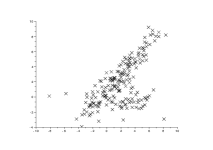
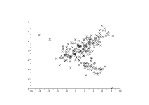
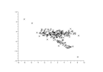
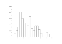
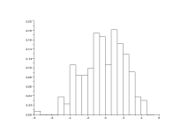
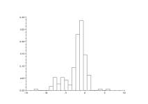
Figure 1: First row: resp. plot of an original data $(X_{i},Y_{i})_{1\leq i\leq n}$ according to model (7) with $n=200$, plot of a wrong $\theta$-tranformation ($\theta\neq\theta^{*}$), plot of the true $\theta^{*}$-tranformation. Second row: resp. histograms of the corresponding first row 2nd-coordinate sample data.

These figures are completed by adding their corresponding 2nd-coordinate sample data histograms. Note that these histograms are empirical estimates of the densities $f_{\theta}$, by formula (12), with $\theta$ respectively equal to $(0,0)$, $(1,0.5)$ and $(2,1)$. We see clearly through these three situations how a progressive transformation of the data allows one to reach a tractable situation in the sense that it looks strongly like the semiparametric contamination model (9) studied in [3] and [5] where a known density is mixed with a symmetric unknown density, which corresponds to the behavior observed in the second row, third column histogram in Fig. 1. Loosely speaking the second idea of our method consists in arguing that once $\theta$ is close to $\theta_{*}$ we are allowed to estimate the proportion $p$ according to a [5] type-method which corresponds to the minimization step (25). In contrast to this technically satisfying idea, the $\theta$-transformation and the choice of the weight distribution $Q$ introduced in (17) are two sources of serious difficulties. In fact when $\beta_{*}$ is large and the law of the design data has heavy tails with respect to the tails of $f$, then the $\theta_{*}$ transformation will move the points coming from the $F_{0}$-population and located far from the origin, to extremely distant positions, which implies intuitively that the integral type density involved in (7) should be extremely heavily tailed. Thus in order to capture the information contained in the tails of the $\theta$-transformed data set it is important to weight sufficiently the empirical index of symmetry $H^{2}(x;p,\tilde{F}_{n,\theta},\hat{J}_{n,\theta})$ of expression (18) for large values of $x$, which reduces to choosing an instrumental distribution $Q$ with non-negligible tails with respect to $F_{\theta_{*}}$.

4.2 Otimization procedure and simulation study

The aim of this section is to illustrate graphically, on a two-dimensionnal examples, the behavior of the empirical distance $d_{n}(p,0,\beta)$ (the parameter $\alpha$ is assumed to be equal to zero) when $p$ and $\beta$ lie close to the true value of the parameter. For simplicity the parameter will still be denoted $\vartheta:=(p,\beta)$, with $\theta:=\beta$ and $d_{n}(\vartheta):=d_{n}(p,0,\beta)$. The interest of this study is to understand closely the influence of the mixing proportion $p$ and the regression coefficient $\beta$ on the shape of the contrast function $d$ (flatness, sharpness, smoothness, etc.). Our models are denoted M1 and M2 and defined according to (6) as follows

M1: $p_{*}=0.7$, $\beta_{*}=1$, $V\sim Q={\mathcal{N}}(0,4^{2})$, $\varepsilon^{[j]}\sim{\mathcal{N}}(0,1)$, $X\sim{\mathcal{N}}(0,3^{2})$,

M2: $p_{*}=0.3$, $\beta_{*}=1$, $V\sim Q={\mathcal{N}}(0,2^{2})$, $\varepsilon^{[j]}\sim{\mathcal{N}}(0,1)$, $X\sim{\mathcal{N}}(0,3^{2})$,

where $j=0$, 1.

In Fig. 2 we plot the mapping $(p,\beta)\mapsto d_{n}(p,\beta)$ obtained from an M1-sample, resp. M2-sample, of size $n=100$, where $(p,\beta)\in\Theta_{1}=[0.5,0.8]\times[0.9,1.1]$, resp. $(p,\beta)\in\Theta_{2}=[0.1,0.6]\times[0.6,1.4]$. Notice that according to discussion (CG) at the end of Section 5.1, model M2 is not necessarily consistently estimated if the parameter space $\Theta_{2}$ contains the spurious solution $\vartheta_{**}=(2p_{*},\beta_{*}/2)$, which is voluntary the case here.

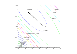
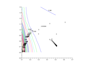
Figure 2: Plot of $(p,\beta)\mapsto d_{n}(p,0,\beta)$ with $n=100$, $\beta_{*}=1$, $\varepsilon_{1}^{[j]}\sim{\mathcal{N}}(0,1),$ $j=0,1$, $X_{1}\sim{\mathcal{N}}(2,3^{2})$, with the difference that on the left hand side $p_{*}=0.7$, $V_{1}\sim{\mathcal{N}}(0,4^{2})$, when on the right hand side $p_{*}=0.3$ $V_{1}\sim{\mathcal{N}}(0,2^{2})$.

In practice, Fig. 2 is obtained using the Scilab contour2d function which plots the level curves of $d_{n}$ evaluated on a homogeneous $10\times 10$ grid of the rectangular domain $[0.5,0.8]\times[0.9,1.1]$. Fig. 2 shows that the graph of $d_{n}$ looks like a sharp valley with a flat trough when $\beta$ is located near $\beta^{*}$ and $p$ ranges [0.5,0.8]. Even if on this simulated example the argmin of $d_{n}$ is very close to the true value of the parameter, the previous remark suggests that the estimation of the mixing proportion will be less robust than the estimation of the regression coefficient. The observation of the second plot in Fig. 2 is more unexpected since the graph of $d_{n}$ does not really look like a contrast function with its high near $p=0.1$ and its very large and flat trough that covers most of $\Theta_{2}$ suggesting a strong lack of robustness of our estimating method in that kind of situation. To validate these thoughts we propose to apply a large sample study on the example and a third intermediary one obtained by considering $p_{*}=0.3$ and $V\sim{\mathcal{N}}(0,4^{2})$. The results of this study will be summarized in Table 1. First we present the numerical approach used to approximate our M-estimator (25).

Gradient algorithm and tuning parameters. The gradient optimization procedure (programmed with Scilab) used to compute our M-estimator $\hat{\vartheta}_{n}=(\hat{p}_{n},\hat{\beta}_{n})$ is defined as follows:

1. Initialization: $\vartheta_{1}=\vartheta_{*}$, $\vartheta_{2}=\vartheta_{*}+\delta$;

2. while $\|\vartheta_{2}-\vartheta_{1}\|_{2}>\epsilon$ do $\vartheta_{1}=\vartheta_{2}$ and $\vartheta_{2}=\vartheta_{1}-\gamma^{T}\dot{d}_{n}(\vartheta_{1})$;

3. else $\hat{\vartheta}_{n}=\vartheta_{2}$,

where $\delta\in\mathbb{R}^{2}$ is used to create a small perturbation of the initial value, $\epsilon>0$ defines the wanted stabilization level in the stopping algorithm procedure, and $\gamma\in{\mathbb{R}^{+*}}^{2}$ is a scale parameter that needs to be hand-tuned for good efficiency in practice (to avoid reverberation phenomena when the score function becomes abruptly sharp). The score function $\dot{d}_{n}:=\left(\frac{\partial}{\partial p}d_{n},\frac{\partial}{\partial\beta}d_{n}\right)^{T}$ can be expressed into a closed form, i.e.

$$\frac{\partial}{\partial p}d_{n}(\vartheta) = 2\int_{\mathbb{R}}h_{n,p}(y,\vartheta)H_{n}(y,\vartheta)dQ_{n}(y),$$

$$\frac{\partial}{\partial\beta}d_{n}(\vartheta) = 2\int_{\mathbb{R}}h_{n,\beta}(y,\vartheta)H_{n}(y,\vartheta)dQ_{n}(y),$$

where for all $y\in\mathbb{R}$,

$$h_{n,p}(y,\vartheta) := \frac{\partial}{\partial p}H_{n}(y,\vartheta)=-\frac{1}{p^{2}}\left(\tilde{F}_{n,\beta}(y)+\tilde{F}_{n,\beta}(-y)-[\hat{J}_{n,\beta}(y)+\hat{J}_{n,\beta}(-y)]\right)$$

$$h_{n,\beta}(y,\vartheta) := \frac{\partial}{\partial\beta}H_{n}(y,\vartheta)=\frac{1}{p}\left(\tilde{\Psi}_{n,\beta}(y)+\tilde{\Psi}_{n,\beta}(-y)\right)-\frac{1-p}{p}\left({j}_{n,\beta}(y)+{j}_{n,\beta}(-y)\right),$$

and where, from (22) and (23)

$$\tilde{\Psi}_{n,\beta}(y) := \frac{\partial}{\partial\beta}\tilde{F}_{n,\beta}(y)$$

$$= \frac{1}{nb_{n}}\sum_{i=1}^{n}\frac{\partial}{\partial\beta}\int_{-\infty}^{y}K\left(\frac{t-(Y_{i}-\beta X_{i})}{b_{n}}\right)dt$$

$$= \frac{1}{n}\sum_{i=1}^{n}\frac{\partial}{\partial\beta}\int_{-\infty}^{\frac{y+\beta X_{i}-Y_{i}}{b_{n}}}K\left(u\right)du$$

$$= \frac{1}{nb_{n}}\sum_{i=1}^{n}X_{i}K\left(\frac{y+\beta X_{i}-Y_{i}}{b_{n}}\right),$$

and similarly, from (21)

$${j}_{n,\beta}(y) := \frac{\partial}{\partial\beta}\hat{J}_{n,\beta}(y)$$

$$= \frac{1}{n}\sum_{i=1}^{n}X_{i}f_{0}\left(y+\beta X_{i}\right).$$

The kernel $K$ used to compute (23), is a triangular kernel defined by

$$K(x)=(1-|x|)\hbox{1\!\!I}_{-1\leq x\leq 1},\quad\quad x\in\mathbb{R},$$

and the bandwidth $b_{n}=\sqrt{1+4p(1-p)}(4/(3n))^{1/5}$ (proposed by [7] for gaussian distributions and implemented in R), both obviously satisfying condition (K). The results summarized in Table 1 were obtained with the following hand-tuned parameters: $\delta=0.01$, $\epsilon=0.005$, $\gamma=(0.2,0.5)^{T}$, and an example of stabilization for this set of tuning parameters is illustrated in Fig 2, where the successive positions (until stabilization) of our algorithm are depicted by cross symbols.

Table 1: Mean and Std. Dev. of 100 estimates of $p$, $\beta$.

$n$ $(p_{*},\beta_{*},\sigma_{V})$ Empirical means Standard deviation 100 (0.7,1,4) (0.7055,1.0051) (0.0373,0.0697) 200 (0.7,1,4) (0.6976,0.9965) (0.0307,0.0590) 500 (0.7,1,4) (0.6954,1.0059) (0.0296,0.0358) 100 (0.3,1,4) (0.3100,0.9581) (0.0577,0.1252) 200 (0.3,1,4) (0.2965,0.9851) (0.0501,0.0855 ) 500 (0.3,1,4) (0.2975,1.0178) (0.0284,0.0414) 100 (0.3,1,2) (0.3971, 0.8587) (0.0942, 0.2213) 200 (0.3,1,2) (0.3982,0.9149) (0.0835,0.1900) 500 (0.3,1,2) (0.3315, 0.9683) (0.0524, 0.1067)

Comments on Table 1. First of all, it is interesting to compare the performances summarized in rows 1–3 of Table 1 to those obtained in [5], p. 35, Table 1 where the model of interest is (9), with $p=0.7$, $\mu=3$, and $f_{0}$ and $f$ are respectively the pdfs corresponding to the $\mathcal{N}(0,1)$ and $\mathcal{N}(0,(1/2)^{2})$ distributions. Even if these two models are not strictly comparable we think that it is interesting, in order to highlight the drawbacks induced by the $\theta$-transformation and the choice of $Q$ discussed above, to compare pairwise the performance obtained on the mixing proportion $p$ and the parameters that influence the location of the $F$-population, i.e. $\beta$ and $\mu$. From the numerical point of view, we easily check that the bias of our estimators, for both models, is negligible. However it also appears that the standard deviation associated to $(\hat{p}_{n},\hat{\beta}_{n})$ decreases significantly slower than the standard deviation associated to $(\hat{p}_{n},\hat{\mu}_{n})$ when $n$ grows. The performance summarized in rows 4–6 of Table 1, which corresponds to $p=0.3$ (and hence signifies that the population that will move far from its original position due to the $\theta$-transformation will be more important), is very instructive. We observe that for small $n$ ($n=100$, 200) the standard deviations associated to $(\hat{p}_{n},\hat{\beta}_{n})$ are dramatically large compared to those obtained with $p=0.7$. Let $\mbox{std}(n,p_{*},\beta_{*},\sigma_{V})$ the couple of standard deviations calculated in the last column of Table 1 under $(n,p_{*},\beta_{*},\sigma_{V})$. If we compute componentwise the ratios $\mbox{std}(n,0.3,1,4)/\mbox{std}(n,0.7,1,4)$ respectively for $n=100,200,500$ we obtain approximately $(1.54,1.8)$, $(1.67,1.44)$, and $(0.95,1.17)$ which seems to suggest that when $n$ becomes large the side effect of the $\theta$-transformation vanishes (probably thanks to the size of $n$, which increases globally the precision of the empirical estimates, and the tails of $Q$, that allow the algorithm to take these improvements into account efficiently). The performances summarized in rows 7–9 of Table 1, seems to confirm the concerns expressed about model M2. We recall that model M2 is badly affected by the two following drawbacks : smallness of $p_{*}$ (synonymous with important population shifted far by the $\theta$-transformation and existence of a spurious solution) and a smallness of $\sigma_{V}$ which is then clearly not sufficient to counteract the smallness of $p_{*}$ (and its consequences). We think in particular that, in model M2, the empirical contrast $d_{n}$ is more easily closer to 0 under $\beta_{**}=\beta_{*}/2$ since as explained in Section 4.1., this value is then significantly smaller than $\beta_{*}$. This last remark explains why, in spite of the fact that our algorithms were initialized at the true parameter value, our estimates are strongly biased (attracted quite often by the spurious solution $\vartheta_{**}$).

Robustness with respect to the symmetry assumption. We propose to conclude this simulation study by testing our method in situations where the law of the error $\varepsilon^{[1]}$ is no longer symmetric. For this purpose we consider again model M1 and replace the distribution of $\varepsilon^{[1]}$ by the mixture

$$\lambda{\mathcal{N}}(-0.7,1/\sqrt{2})+(1-\lambda){\mathcal{N}}(0.7\lambda/(1-\lambda),1/\sqrt{2})$$

which pdf, denoted $f_{\lambda}$, is nonsymmetric if $\lambda\neq 0.5$ but has a mean equal to 0 and a variance equal to 0.5 for all $\lambda\in(0,1)$. In our simulations we consider successively $\lambda=0.5,0.55,0.6$ which leads to consider pdfs for $\varepsilon^{[1]}$ which graphs are plotted in Fig 3.

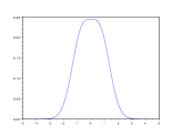
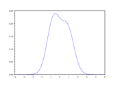
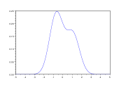
Figure 3: Graphs of the pdfs corresponding to the mixture distribution $\lambda{\mathcal{N}}(-0.7,1/\sqrt{2})+(1-\lambda){\mathcal{N}}(0.7\lambda/(1-\lambda),1/\sqrt{2})$, obtained by considering $\lambda=0.5,0.55,0.6$.

Some performances of our method on these examples are summarized in Table 2.

Table 2: Mean and Std. Dev. of 100 estimates of $p$, $\beta$.

$n$ $\lambda$ Empirical means Standard deviation 100 0.5 (0.7035,1.0229) (0.0427,0.0814) 200 0.5 (0.7012,1.0068) (0.0390,0.0774) 500 0.5 (0.6997,1.0059) (0.0244,0.0488) 100 0.55 (0.6854,1.0837) (0.0485,0.0858) 200 0.55 (0.6890,1.0805) (0.0431,0.0716) 500 0.55 (0.6922,1.0699) (0.0377,0.0519) 100 0.6 (0.6731,1.1314) (0.0543,0.0952) 200 0.6 (0.6693,1.1061) (0.0490,0.0868) 500 0.6 (0.6775,1.0928) (0.0392,0.0557)

Comments on Table 2. Note that when $\lambda=0.5$ (symmetric case) the performances of our method are very close to those obtain on model M1. However for $n=100,200$ the standard deviation of our estimates is larger than those obtained in the M1 model, when for $n=500$ the standard deviation becomes slightly smaller. This behavior can probably be explained by the fact that the graph of $f_{0.5}$ is flat on its top which intuitively do not help much in locating the axis of symmetry for small values of $n$. On the other hand we can expect that for $n=500$, helped with the fact that $\mbox{var}(\varepsilon^{[1]})$ is here equal to $0.5$ when it was equal to $1$ in M1, our nonparametric estimators perform better than in model M1 which should explain the good performances observe in the third row of Table 2. When $\lambda=0.55,0.6$ it appears that the parameter $\beta$ is always overestimated. This phenomenon can be explained by the fact that our method try to determine a pseudo-axis of symmetry adapted to the shapeless graph of $f_{\lambda}$ which qualitatively is placed on the left side of the origin. This remark implies that the $\theta$-transformation needed to transform the first integral in (12) into an almost even density (see Fig. 2) have to contain a $\beta$ greater than $\beta_{*}$.

5 Appendix

5.1 Conditions (R) and (C) in the Gaussian Case

In this section we discuss conditions (R) and (C) when the true underlying model is a contaminated Gaussian regression model with Gaussian design, i.e., $f$, $f_{0}$, $h$ are respectively the pdfs of the ${\mathcal{N}}(0,m)$, ${\mathcal{N}}(0,m_{0})$, and ${\mathcal{N}}(E(X),\sigma_{h}^{2})$ distributions.

Comments on condition (R). Conditions (R) i-iii) are standard and easy to verify in the above model. On the other hand, it is interesting to show how conditions (R) iv-v) arise naturally in this case.

Condition (R) iv). We show for simplicity that the first condition in (R) iv) (the same kind of proof works also for the second one) holds when $i=0$, $\theta^{*}=(\alpha_{*},\beta_{*})\in{\mathbb{R}^{+*}}^{2}$ and $m_{0}=1$. We write the decomposition

$$|F_{0}(y+\theta_{*}\odot x)-F_{0}(y-\theta_{*}\odot x)|=$$

$$~{}~{}~{}~{}~{}~{}~{}~{}~{}~{}~{}~{}~{}~{}~{}~{}~{}|F_{0}(y+\theta_{*}\odot x)-F_{0}(y-\theta_{*}\odot x)|\hbox{1\!\!I}_{y>1-\theta_{*}\odot x,~{}x<-\frac{\alpha_{*}}{\beta_{*}}}$$

$$~{}~{}~{}~{}~{}~{}~{}~{}~{}~{}~{}~{}~{}+|F_{0}(y+\theta_{*}\odot x)-F_{0}(y-\theta_{*}\odot x)|\hbox{1\!\!I}_{y>1+\theta_{*}\odot x,~{}x\geq-\frac{\alpha_{*}}{\beta_{*}}}$$

$$~{}~{}~{}~{}~{}~{}~{}~{}~{}~{}~{}~{}~{}+|F_{0}(y+\theta_{*}\odot x)-F_{0}(y-\theta_{*}\odot x)|\hbox{1\!\!I}_{y<-1+\theta_{*}\odot x,~{}x<-\frac{\alpha_{*}}{\beta_{*}}}$$

$$~{}~{}~{}~{}~{}~{}~{}~{}~{}~{}~{}~{}~{}+|F_{0}(y+\theta_{*}\odot x)-F_{0}(y-\theta_{*}\odot x)|\hbox{1\!\!I}_{y<-1-\theta_{*}\odot x,~{}x\geq-\frac{\alpha_{*}}{\beta_{*}}}$$

$$~{}~{}~{}~{}~{}~{}~{}~{}~{}~{}~{}~{}~{}+|F_{0}(y+\theta_{*}\odot x)-F_{0}(y-\theta_{*}\odot x)|\hbox{1\!\!I}_{-1+\theta_{*}\odot x\leq y\leq 1-\theta_{*}\odot x,~{}x<-\frac{\alpha_{*}}{\beta_{*}}}$$

$$~{}~{}~{}~{}~{}~{}~{}~{}~{}~{}~{}~{}~{}+|F_{0}(y+\theta_{*}\odot x)-F_{0}(y-\theta_{*}\odot x)|\hbox{1\!\!I}_{-1-\theta_{*}\odot x\leq y\leq 1+\theta_{*}\odot x,~{}x\geq-\frac{\alpha_{*}}{\beta_{*}}}.$$

Consider the first term on the right hand side of the above decomposition (the three following terms being treated in entirely same way). For all $y>1-\theta_{*}\odot x$ with $x<-\alpha_{*}/\beta_{*}$ we have $y-\theta_{*}\odot x>y+\theta_{*}\odot x>1$. Since for $t>0$ large enough, the inequality (53) is valid

$$\frac{\exp(-t^{2})}{\sqrt{2\pi}}\left(\frac{1}{t}-\frac{1}{t^{3}}\right)\leq 1-F_{0}(t)\leq\frac{\exp(-t^{2})}{t\sqrt{2\pi}},$$ (53)

we have in particular that for all $t>1$, $0\leq 1-F_{0}(t)\leq\exp(-t^{2})/\sqrt{2\pi}$. Hence it follows that for $y>1-\theta_{*}\odot x$ with $x<-\alpha_{*}/\beta_{*}$:

$$|F_{0}(y+\theta_{*}\odot x)-F_{0}(y-\theta_{*}\odot x)|\leq\frac{\exp(-(y+\theta_{*}\odot x)^{2})+\exp(-(y-\theta_{*}\odot x)^{2})}{\sqrt{2\pi}},$$

which proves that this first term is $h(x)dxdy$ integrable. Let us now sum the last two terms of the above decomposition and notice that

$$|F_{0}(y+\theta_{*}\odot x)-F_{0}(y-\theta_{*}\odot x)|$$

$$\times\left(\hbox{1\!\!I}_{-1+\theta_{*}\odot x\leq y\leq 1-\theta_{*}\odot x,~{}x<-\frac{\alpha}{\beta_{*}}}+\hbox{1\!\!I}_{-1-\theta_{*}\odot x\leq y\leq 1+\theta_{*}\odot x,~{}x\geq-\frac{\alpha}{\beta_{*}}}\right)$$

$$\leq 2\hbox{1\!\!I}_{-1-|\theta_{*}\odot x|\leq y\leq 1+|\theta_{*}\odot x|}.$$

We thus prove that this sum of terms is also $h(x)dxdy$ integrable.

Condition (R) v). We consider for simplicity the construction of the bounding function $\ell^{0}_{1,1}$ when $(\alpha,\beta)\in\Phi=[\underline{\alpha},\overline{\alpha}]\times[\underline{\beta},\overline{\beta}]$, with $(\underline{\alpha},\underline{\beta})\in{\mathbb{R}^{+*}}^{2}$ and $m=m_{0}=1$. Notice first that for all $(x,y)\in\mathbb{R}^{2}$

$$|f_{0}^{(1)}(y+\theta\odot x)|\leq\frac{|y|+\overline{\alpha}+\overline{\beta}|x|}{\sqrt{2\pi}}\exp\left(-\frac{(y+\alpha+\beta x)^{2}}{2}\right).$$

Secondly it is easy to check that for all $(x,y)\in\mathbb{R}^{2}$ and all $\theta\in\Phi$:

$$\exp\left(-\frac{(y+\alpha+\beta x)^{2}}{2}\right)$$

$$~{}~{}~{}~{}~{}~{}~{}~{}~{}~{}~{}~{}~{}~{}~{}~{}~{}\leq\exp\left(-\frac{(y+\underline{\beta}x)^{2}}{2}\right)\hbox{1\!\!I}_{x\geq 0,y\geq 0}$$

$$~{}~{}~{}~{}~{}~{}~{}~{}~{}~{}~{}~{}~{}~{}~{}~{}~{}~{}+\exp\left(-\frac{\min(|y+\underline{\alpha}+\underline{\beta}x|,|y+\overline{\alpha}+\overline{\beta}x|)^{2}}{2}\right)\hbox{1\!\!I}_{x\geq 0,y\leq 0}$$

$$~{}~{}~{}~{}~{}~{}~{}~{}~{}~{}~{}~{}~{}~{}~{}~{}~{}~{}+\exp\left(-\frac{\min(|y+\underline{\alpha}+\overline{\beta}x|,|y+\overline{\alpha}+\underline{\beta}x|)^{2}}{2}\right)\hbox{1\!\!I}_{x\leq 0,y\in\mathbb{R}}$$

$$~{}~{}~{}~{}~{}~{}~{}~{}~{}~{}~{}~{}~{}~{}~{}~{}~{}\leq B_{\Phi}(x,y),$$

where

$$B_{\Phi}(x,y) := \exp\left(-\frac{(y+\underline{\beta}x)^{2}}{2}\right)+\exp\left(-\frac{(y+\underline{\alpha}+\underline{\beta}x)^{2}}{2}\right)$$

$$+\exp\left(-\frac{(y+\overline{\alpha}+\overline{\beta}x)^{2}}{2}\right)+\exp\left(-\frac{(y+\underline{\alpha}+\overline{\beta}x)^{2}}{2}\right)$$

$$+\exp\left(-\frac{(y+\overline{\alpha}+\underline{\beta}x)^{2}}{2}\right).$$

Thus we can propose $\ell^{0}_{1,1}(x,y)=|x|(|y|+\overline{\alpha}+\overline{\beta}|x|)/\sqrt{2\pi}B_{\Phi}(x,y)\exp(-x^{2}/2)$, which clearly belongs to $L_{1}(\mathbb{R}^{2})$, as a candidate for the uniformly bounding function satisfying condition (R) v).

Comments on condition (C). In the whole Gaussian case, expression of (39) becomes:

$$p_{*}\sin((\alpha-\alpha_{*})+(\beta-\beta_{*})E(X))t)\exp\left(-\frac{t^{2}}{2}(\sigma_{h}^{2}(\beta-\beta_{*})^{2}+m)\right)$$

$$~{}~{}~{}~{}~{}~{}~{}~{}~{}~{}=(p_{*}-p)\sin((\alpha+\beta E(X))t)\exp\left(-\frac{t^{2}}{2}(\sigma_{h}^{2}\beta^{2}+m_{0})\right).$$ (54)

We suppose first that $p\neq p_{*}$, and denote $\xi:=\alpha+\beta E(X)$, $\xi_{*}:=\alpha_{*}+\beta_{*}E(X)$, $\Sigma_{\beta-\beta_{*}}:=\sigma_{h}^{2}(\beta-\beta_{*})^{2}+m$, and $\Sigma_{\beta}:=\sigma_{h}^{2}\beta^{2}+m_{0}$. Taking the first and third order derivative of (5.1) at point $t=0$ we get the conditions

$$p_{*}\xi_{*}=p\xi,\quad\mbox{and}\quad(p-p_{*})\xi(3\Sigma_{\beta-\beta_{*}}+\xi^{2})+p_{*}(\xi-\xi_{*})(3\Sigma_{\beta}+(\xi-\xi_{*})^{2})=0.$$ (55)

Introducing the first relation in (55) into the second one, we obtain

$$\frac{p-p_{*}}{p}\xi_{*}p_{*}\left(3[\Sigma_{\beta}-\Sigma_{\beta-\beta_{*}}]+\frac{2p_{*}p-p^{2}}{p^{2}}\xi_{*}^{2}\right)=0.$$ (56)

Now we observe that, to insure the validity of expression (5.1), the factors multiplied by the $\sin$ terms on both sides of (5.1) must be, at least, equivalent as $t\rightarrow\infty$. This last remark implies that $\Sigma_{\beta}=\Sigma_{\beta-\beta_{*}}$, or equivalently $\beta=\beta_{*}/2+(m_{0}-m)/2\beta_{*}\sigma_{h}^{2}$, and thus (56) leads to

$$p=2p_{*}.$$ (57)

Using now the first relation in (5.1) and (57), we then obtain $\alpha=\alpha_{*}/2+E(X)(m_{0}-m)/2\beta_{*}\sigma_{h}^{2}$.

The consequences of the previous comments can be presented as follows:

Discussion (CG):

1. If $p_{*}>1/2$ then the set of parameters $\vartheta\in\Theta$ satisfying condition (5.1) is always empty, since $p=2p^{*}>1$ is not an admissible solution.

2. If $p_{*}\leq 1/2$ and if, for example, $E(X)=0$ and $m_{0}=m$ then $\vartheta_{**}=(2p^{*},\alpha_{*}/2,\beta_{*}/2)$. In such a case it would be crucial to build a conveniently constrained parametric space (most of the time a plot of the dataset helps in building reasonnable constraints on the intercept and slope parameter spaces) expecting that it contains $\vartheta_{*}$ but not $\vartheta_{**}$.

3. More generaly one can expect that when the shape of the sample data (see e.g. Fig. 1) suggest that $(m_{0}-m)/2\beta_{*}\sigma_{h}^{2}$ is negligible with respect to $\alpha_{*}$ and $\beta_{*}$, which occurs when $m_{0}$ is close to $m$ or/and $\sigma_{h}^{2}\beta_{*}$ is very large, then the solution proposed in ii) is loosely speaking still valid.

5.2 Explicit formula of $H(\cdot,\vartheta)$ and its derivatives

In this section all the expressions are valid for all $(\vartheta,y)\in\Theta\times\mathbb{R}$, and the computation of the various derivative functions (under the integral sign) are all allowed according to Lebesgue’s Theorem and condition (R). According to (12) and (14), we have

$$H(y,\vartheta) = \frac{p^{*}}{p}\left(\int_{-\infty}^{y}\int_{\mathbb{R}}f(z+(\theta-\theta^{*})\odot x)h(x)dxdz\right.$$

$$+\left.\int_{-\infty}^{-y}\int_{\mathbb{R}}f(z+(\theta-\theta^{*})\odot x)h(x)dxdz\right)$$

$$+\frac{p-p^{*}}{p}\left(\int_{-\infty}^{y}\int_{\mathbb{R}}f_{0}(z+\theta\odot x)h(x)dxdz\right.$$

$$+\left.\int_{-\infty}^{-y}\int_{\mathbb{R}}f_{0}(z+\theta\odot x)h(x)dxdz\right)-1.$$

For simplicity we introduce

$$F^{\theta}(y) = \int_{-\infty}^{y}\int_{\mathbb{R}}f(z+(\theta-\theta^{*})\odot x)h(x)dxdz,$$

$$F_{0}^{\theta}(y) = \int_{-\infty}^{y}\int_{\mathbb{R}}f_{0}(z+\theta\odot x)h(x)dxdz,$$

which leads to

$$\frac{\partial}{\partial p}H(y,\vartheta)=-\frac{p^{*}}{p^{2}}\left[(F^{\theta}(y)+F^{\theta}(-y))-(F_{0}^{\theta}(y)+F_{0}\theta(-y))\right].$$

Let us denote

$$\dot{F}^{\alpha}(y) := \frac{\partial}{\partial\alpha}F^{\theta}(y)=\int_{-\infty}^{y}\int_{\mathbb{R}}\dot{f}(z+(\theta-\theta_{*})\odot x)h(x)dxdz,$$

$$\dot{F}_{0}^{\alpha}(y) := \frac{\partial}{\partial\alpha}F_{0}^{\theta}(y)=\int_{-\infty}^{y}\int_{\mathbb{R}}\dot{f}_{0}(z+\theta\odot x)h(x)dxdz,$$

and for

$$\dot{F}^{\beta}(y) := \frac{\partial}{\partial\beta}F\theta(y)=\int_{-\infty}^{y}\int_{\mathbb{R}}x\dot{f}(z+(\theta-\theta^{*})\odot x)h(x)dxdz,$$

$$\dot{F}_{0}^{\beta}(y) := \frac{\partial}{\partial\beta}F_{0}\theta(y)=\int_{-\infty}^{y}\int_{\mathbb{R}}x\dot{f}_{0}(z+\theta\odot x)h(x)dxdz,$$

we obtain

$$\frac{\partial}{\partial\alpha}H(y,\vartheta)=\frac{p^{*}}{p}\left(\dot{F}^{\alpha}(y)+\dot{F}^{\alpha}(-y)\right)+\frac{p-p^{*}}{p}\left(\dot{F}_{0}^{\alpha}(y)+\dot{F}_{0}^{\alpha}(-y)\right).$$

$$\frac{\partial}{\partial\beta}H(y,\vartheta)=\frac{p^{*}}{p}\left(\dot{F}^{\beta}(y)+\dot{F}^{\beta}(-y)\right)+\frac{p-p^{*}}{p}\left(\dot{F}_{0}^{\beta}(y)+\dot{F}_{0}^{\beta}(-y)\right).$$

At point $\vartheta=\vartheta_{*}$ the Hessian matrix of $H(\cdot,\vartheta)$ defined in (44) is obtained by considering

$$\dot{H}(y,\vartheta_{*})=\left(\begin{array}[]{c}\displaystyle{\frac{1}{p}\left(F_{0}^{\theta_{*}}(y)+F_{0}^{\theta_{*}}(-y)-1\right)}\\ 2f(y)\\ 2f(y)E(X)\end{array}\right).$$ (61)

Let us denote now

$$\ddot{F}^{\beta,\alpha}(y)=\frac{\partial^{2}}{\partial\beta\partial\alpha}F^{\theta}(y) = \int_{-\infty}^{y}\int_{\mathbb{R}}x\ddot{f}(z+(\theta-\theta_{*})\odot x)h(x)dxdz,$$

$$\ddot{F}_{0}^{\beta,\alpha}(y)=\frac{\partial^{2}}{\partial\beta\partial\alpha}F_{0}^{\theta}(y) = \int_{-\infty}^{y}\int_{\mathbb{R}}x\ddot{f}_{0}(z+\theta\odot x)h(x)dxdz,$$

$$\ddot{F}^{\alpha,\alpha}(y)=\frac{\partial^{2}}{\partial\alpha^{2}}F^{\theta}(y) = \int_{-\infty}^{y}\int_{\mathbb{R}}\ddot{f}(z+(\theta-\theta_{*})\odot x)h(x)dxdz,$$

$$\ddot{F}_{0}^{\beta,\beta}(y)=\frac{\partial^{2}}{\partial\beta^{2}}F_{0}^{\theta}(y) = \int_{-\infty}^{y}\int_{\mathbb{R}}x^{2}\ddot{f}_{0}(z+\theta\odot x)h(x)dxdz.$$

We then obtain

$$\frac{\partial^{2}}{\partial p^{2}}H(y,\vartheta) = \frac{p^{*}}{p^{3}}\left[(F^{\theta}(y)+F^{\theta}(-y))-(F_{0}^{\theta}(y)+F_{0}\theta(-y))\right],$$

$$\frac{\partial^{2}}{\partial u\partial p}H(y,\vartheta) = -\frac{p^{*}}{p^{2}}\left[(\dot{F}^{u}(y)+\dot{F}^{u}(-y))-(\dot{F}_{0}^{u}(y)+\dot{F}_{0}^{u}(-y))\right],\quad u=\alpha,~{}\beta,$$

$$\frac{\partial^{2}}{\partial u\partial v}H(y,\vartheta) = \frac{p^{*}}{p}\left(\ddot{F}^{u,v}(y)+\ddot{F}^{u,v}(-y)\right)$$

$$+\frac{p-p^{*}}{p}\left(\ddot{F}_{0}^{u,v}(y)+\ddot{F}_{0}^{u,v}(-y)\right),\quad u=\alpha,~{}\beta,\quad v=\alpha,~{}\beta.$$

5.3 Boundedness

Boundedness of $\Psi_{\theta}(\cdot)$ and $\Psi^{\prime}_{\theta}(\cdot)$. If $f$ and $f_{0}$ are supposed to be bounded over $\mathbb{R}$ then we clearly have from (12) that

$$|\Psi_{\theta}(y)|\leq\|f\|_{\infty}+\|f_{0}\|_{\infty},\quad\quad(\theta,y)\in\Phi\times\mathbb{R}.$$

The same kind of argument holds to prove boundedness of $\dot{f}_{\theta}(\cdot)$ when (R) ii) is supposed.

Boundedness of $H(\cdot,\vartheta)$. Since for all $\theta\in\Phi$ the functions $F_{\theta}(\cdot)$ and $J_{\theta}(\cdot)$ are both cdfs, we thus have, since $\delta\leq p\leq 1-\delta$, from expression (16):

$$H(y,\vartheta)\leq\frac{4}{\delta}+1,\quad\quad(y,\vartheta)\in\mathbb{R}\times\Phi.$$ (62)

5.4 Integrable Lipschitz property of $\Psi_{\theta}(\cdot)$

From (12), for all $(y,\theta,\theta^{\prime})\in\mathbb{R}\times\Phi^{2}$ we have

$$|\Psi_{\theta}(y)-f\Psi_{\theta^{\prime}}(y)| \leq p_{*}\int_{\mathbb{R}}|f(y+(\theta-\theta_{*})\odot x)-f(y+(\theta^{\prime}-\theta_{*})\odot x)|h(x)dx$$ (63)

$$+(1-p_{*})\int_{\mathbb{R}}|f_{0}(y+\theta\odot x)-f_{0}(y+\theta^{\prime}\odot x)|h(x)dx.$$

Consider for simplicity the first integral term on the right hand side of (63) (the same argument holding for the second term). According to the Mean Value Theorem there exists, for all $(x,y)\in\mathbb{R}^{2}$ and $(\theta,\theta^{\prime})\in\Phi^{2}$, a value $\gamma:=\gamma(x,y,\theta,\theta^{\prime})$ belonging to the line segment with extremities $y+(\theta-\theta_{*})\odot x$ and $y+(\theta^{\prime}-\theta_{*})\odot x$, or equivalently a $\bar{\theta}:=\bar{\theta}(x,y,\theta,\theta^{\prime})$ belonging to the line segment with extremities $\theta$ and $\theta^{\prime}$ such that $\gamma=y+(\bar{\theta}-\theta_{*})\odot x$ and

$$|f(y+(\theta-\theta_{*})\odot x)-f(y+(\theta^{\prime}-\theta_{*})\odot x)|$$

$$~{}~{}~{}~{}~{}~{}~{}~{}~{}~{}~{}~{}~{}~{}=|\dot{f}(\gamma)(\alpha-\alpha^{\prime}+(\beta-\beta^{\prime})x)|$$

$$~{}~{}~{}~{}~{}~{}~{}~{}~{}~{}~{}~{}~{}~{}=|\dot{f}(y+(\bar{\theta}-\theta_{*})\odot x)(\alpha-\alpha^{\prime}+(\beta-\beta^{\prime})x)|$$

$$~{}~{}~{}~{}~{}~{}~{}~{}~{}~{}~{}~{}~{}~{}\leq\sup_{\theta\in\Phi}|\dot{f}(y+(\theta-\theta_{*})\odot x)|(|\alpha-\alpha^{\prime}|+|\beta-\beta^{\prime}||x|).$$

From condition (R) ii) there thus exists a nonnegative constant $c$ such that

$$\int_{\mathbb{R}}|\Psi_{\theta}(y)-\Psi_{\theta^{\prime}}(y)|$$

$$\leq\sum_{j=0,1}(|\alpha-\alpha^{\prime}|^{1-j}+|\beta-\beta^{\prime}|^{j})$$

$$\int_{\mathbb{R}\times\mathbb{R}}|x|^{j}(\sup_{\theta\in\Phi}|\dot{f}(z+(\theta-\theta_{*})\odot x)|+\sup_{\theta\in\Phi}|\dot{f}_{0}(z+\theta\odot x)|)h(x)dxdz$$

$$\leq c\|\theta-\theta^{\prime}\|_{2}.$$

5.5 Uniform Lipschitz property of $H(\cdot,\vartheta)$

Let us write

$$H(y,\vartheta)-H(y,\vartheta^{\prime})$$

$$= \frac{1}{p}\left(F_{\theta}(y)-F_{\theta^{\prime}}(y)+F_{\theta}(-y)-F_{\theta^{\prime}}(-y)\right)+\frac{p-p^{\prime}}{pp^{\prime}}(F_{\theta^{\prime}}(y)+F_{\theta^{\prime}}(y))$$

$$+\frac{1-p}{p}\left(J_{\theta}(y)-J_{\theta^{\prime}}(y)+J_{\theta}(-y)-J_{\theta^{\prime}}(-y)\right)+\frac{p-p^{\prime}}{pp^{\prime}}(J_{\theta^{\prime}}(y)+J_{\theta^{\prime}}(-y)).$$

To prove the uniform Lipschitz property of $H(\cdot,\vartheta)$ we need to prove it for $J_{\theta}(\cdot)$ and $F_{\theta}(\cdot)$. We begin with the simplest term $J_{\theta}(\cdot)$. According again to the mean value theorem, for all $y\in\mathbb{R}$, all $(x,z)\in\mathbb{R}^{2}$ with $z\leq y$, and all $(\theta,\theta^{\prime})\in\Phi^{2}$ there exists $\bar{\theta}:=\bar{\theta}(x,z,\theta,\theta^{\prime})$ belonging to the line segment with extremities $\theta$ and $\theta^{\prime}$ such that

$$|J_{\theta}(y)-J_{\theta^{\prime}}(y)| \leq \int_{-\infty}^{y}\int_{\mathbb{R}}|f_{0}(z+\theta\odot x)-f_{0}(z+(\theta^{\prime}\odot x)|h(x)dxdz$$

$$= \int_{-\infty}^{y}\int_{\mathbb{R}}|\dot{f}_{0}(z+\bar{\theta}\odot x)(|\alpha-\alpha^{\prime}|+|\theta-\theta^{\prime}||x|)h(x)dxdz,\quad\quad$$

$$\leq \int_{-\infty}^{y}\int_{\mathbb{R}}\sup_{\theta\in\Phi}|\dot{f}_{0}(z+\theta\odot x)h(x)dxdz|\alpha-\alpha^{\prime}|$$

$$+\int_{-\infty}^{y}\int_{\mathbb{R}}|x|\sup_{\theta\in\Phi}|\dot{f}_{0}(z+ux)h(x)dxdz|\beta-\beta^{\prime}|$$

$$\leq c\|\theta-\theta^{\prime}\|_{2},$$

where $c$ denotes a nonnegative constant arising from condition (R) ii). Using the same kind of argument we prove that there exists a nonnegative contant $c^{\prime}$ such that for all $(y,\theta,\theta^{\prime})\in\mathbb{R}\times\Phi^{2}$

$$|F_{\theta}(y)-F_{\theta^{\prime}}(y)|\leq c^{\prime}\|\theta-\theta^{\prime}\|_{2}.$$

In conclusion, for all $y\in\mathbb{R}$, there exists a nonnegative constant $c^{\prime\prime}$ such that for all $(y,\vartheta,\vartheta^{\prime})\in\mathbb{R}\times\Theta^{2}$

$$|H(y,\vartheta)-H(y,\vartheta^{\prime})|\leq\frac{2}{\delta}(c+c^{\prime})\|\theta-\theta^{\prime}\|_{2}+4\frac{|p-p^{\prime}|}{\delta^{2}}\leq c^{\prime\prime}\|\vartheta-\vartheta\|_{3}.$$

5.6 Uniform almost sure rate of convergence of $d_{n}$

Let us consider

$$|d_{n}(\vartheta)-d(\vartheta)|\leq T_{1,n}(\vartheta)+T_{2,n}(\vartheta),$$

where

$$T_{1,n}(\vartheta) := \left|\frac{1}{n}\sum_{i=1}^{n}H^{2}(V_{i};\vartheta,\tilde{F}_{n,\theta},\hat{J}_{n,\theta})-H^{2}(V_{i};\vartheta,F_{\theta},J_{\theta})\right|,$$

$$T_{2,n}(\vartheta) := \left|\frac{1}{n}\sum_{i=1}^{n}H^{2}(V_{i};\vartheta,F_{\theta},J_{\theta})-E\left(H^{2}(V_{1};\vartheta,F_{\theta},J_{\theta})\right)\right|.$$

Uniform almost sure rate of convergence of $T_{1,n}$. Note first that from boundedness of $H(\cdot;\vartheta,\tilde{F}_{n,\theta},\hat{J}_{n,\theta})$ and $H(\cdot;\vartheta,F_{\theta},J_{\theta})$ given by (62), there exist nonnegative constants $C$ and $C^{\prime}$ such that

$$T_{1,n}(\vartheta) = \left|\frac{1}{n}\sum_{i=1}^{n}(H(V_{i};\vartheta,\tilde{F}_{n,\theta},\hat{J}_{n,\theta})+H(V_{i};\vartheta,F_{\theta},J_{\theta}))\right.$$

$$\left.\times(H(V_{i};\vartheta,\tilde{F}_{n,\theta},\hat{J}_{n,\theta})-H(V_{i};\vartheta,F_{\theta},J_{\theta}))\right|$$

$$\leq C\sup_{y\in\mathbb{R}}|H(y;\vartheta,\tilde{F}_{n,\theta},\hat{J}_{n,\theta})-H(y;\vartheta,F_{\theta},J_{\theta}))|$$

$$\leq C^{\prime}\left(\sup_{y\in\mathbb{R}}|\hat{J}_{n,\theta}(y)-J_{\theta}(y)|+\sup_{y\in\mathbb{R}}|\tilde{F}_{n,\theta}(y)-F_{\theta}(y)|\right).$$

Let us now denote

$$T^{(1)}_{1,n} := \sup_{\theta\in\Phi}\sup_{y\in\mathbb{R}}|\hat{J}_{n,\theta}(y)-J_{\theta}(y)|,$$

$$T^{(2)}_{1,n} := \sup_{\theta\in\Phi}\sup_{y\in\mathbb{R}}|\tilde{F}_{n,\theta}(y)-F_{\theta}(y)|.$$

Convergence rate of $T^{(1)}_{1,n}$. For simplicity we will suppose that $\mbox{proj}_{2}(\Phi)\subset[0,A]$, where $A$ is a nonnegative real number and for all $(x,y)\in\mathbb{R}^{2}$, $\mbox{proj}_{2}:(x,y)\mapsto y$. Let us introduce $P^{X}_{n}=n^{-1}\sum_{i=1}^{n}\delta_{X_{i}}$ the empirical measure associated to the iid sample $(X_{1},\dots,X_{n})$ with common probability distribution $P^{X}$ with pdf and cdf resp. denoted by $h$ and $H$). We use the functionnal notation $Pf=\int fdP$. Notice now that, according to expression (21), we have for all $y\in\mathbb{R}$:,

$$\hat{J}_{n,\theta}(y)-J_{\theta}(y) = \frac{1}{n}\sum_{i=1}^{n}F_{0}(y+\alpha+\beta X_{i})-E(F_{0}(y+\alpha+\beta X))$$

$$= (P_{n}^{X}-P^{X})F_{0}(y+\alpha+\beta~{}\cdot).$$

Let consider the class of functions

$$\mathcal{F}_{0}=\left\{x\mapsto F_{0}(u+\beta x);\quad u\in\mathbb{R},\quad\beta\in[0,A]\right\}.$$

Since

$$(P_{n}^{X}-P^{X})F_{0}(u+\beta~{}\cdot)=(P_{n}^{X}-P^{X})F_{0}(y+\beta(\cdot\vee 0))+(P_{n}^{X}-P^{X})F_{0}(y+\beta(\cdot\wedge 0)),$$

it is enough to study the empirical process indexed by the classes of functions

$$\mathcal{F}^{+}_{0} = \left\{x\mapsto F_{0}(u+\beta(x\vee 0));\quad u\in\mathbb{R},\quad\beta\in[0,A]\right\},$$

$$\mathcal{F}^{-}_{0} = \left\{x\mapsto F_{0}(u+\beta(x\wedge 0));\quad u\in\mathbb{R},\quad\beta\in[0,A]\right\}.$$

For simplicity we denote $\Gamma_{y,\alpha}(x)=F_{0}(y+\alpha(x\vee 0))$ and only consider the class $\mathcal{F}^{+}_{0}$, the class $\mathcal{F}^{-}_{0}$ being treated in a entirely same way. Since $F_{0}$ is a cdf, for $\beta_{1}\leq\beta\leq\beta_{2}$ and $u_{1}\leq u\leq u_{2}$ we have

$$\Gamma_{u_{1},\beta_{1}}(x)\leq\Gamma_{u,\beta}(x)\leq\Gamma_{u_{2},\beta_{2}}(x),\quad\quad x\in\mathbb{R},$$

and, since $F_{0}$ is supposed to be Lipschitz,

$$0\leq\Gamma_{u_{2},\beta_{2}}(x)-\Gamma_{u_{1},\beta_{1}}(x)\leq C(u_{2}-u_{1}+(\beta_{2}-\beta_{1})(x\vee 0)).$$

Let consider now $\varepsilon>0$, and $(\overline{u_{\varepsilon}},\underline{u_{\varepsilon}})\in\mathbb{R}^{2}$ such that

$$F_{0}(\overline{u_{\varepsilon}})\geq 1-\varepsilon,\quad\quad\mbox{and}\quad\quad F_{0}(\underline{u_{\varepsilon}})\leq\varepsilon.$$

Note that $\overline{u_{\varepsilon}}$ and $\underline{u_{\varepsilon}}$ do not depend on $\beta$. For all $N\in\mathbb{N}$, define

$$\underline{u_{\varepsilon}}=u_{1,\varepsilon}\leq u_{2,\varepsilon}\leq\ldots\leq u_{N,\varepsilon}=\overline{u_{\varepsilon}},$$

and consider $N(\varepsilon)$ the smallest integer such that $u_{i,\varepsilon}-u_{i-1,\varepsilon}\leq\varepsilon$ for $i=2,\ldots,N(\varepsilon)$. We denote by $\lceil\cdot\rceil$ the integer part function. For all $\varepsilon$ small enough we clearly have

$$N(\varepsilon)\leq\left\lceil\frac{\overline{u_{\varepsilon}}-\underline{u_{\varepsilon}}}{\varepsilon}\right\rceil\leq 2\frac{\overline{u_{\varepsilon}}-\underline{u_{\varepsilon}}}{\varepsilon}.$$

Let us now define $\alpha_{i,\varepsilon}=\varepsilon(i-1)$, $i=1,\ldots,M(\varepsilon)$, where $M(\varepsilon)=\left\lceil\lceil A+1\rceil/\varepsilon\right\rceil$ and thus $\alpha_{M(\varepsilon),\varepsilon}>A$. Observe in addition that

$$\|\Gamma_{u_{i+1,\varepsilon},\beta_{j+1,\varepsilon}}-\Gamma_{u_{i,\varepsilon},\beta_{j,\varepsilon}}\|^{2}_{2,P^{X}} = c^{2}E\left((u_{i+1,\varepsilon}-u_{i,\varepsilon}+(\beta_{j+1,\varepsilon}-\beta_{j,\varepsilon})(X_{1}\wedge 0))^{2}\right)$$

$$\leq 2c^{2}\varepsilon^{2}+2C^{2}\varepsilon E(X_{1}^{2})$$

$$= 2c^{2}\varepsilon^{2}\left(1+E(X_{1}^{2})\right).$$

Hence the expression

$$[\Gamma_{u_{i+1,\varepsilon},\beta_{j+1,\varepsilon}}-\Gamma_{u_{i,\varepsilon},\beta_{j,\varepsilon}}],\quad 1\leq i\leq N(\varepsilon),\quad 1\leq j\leq M(\varepsilon),$$

is a $\left(c\sqrt{2(1+E(X_{1}^{2}))}\right)$-covering of $\mathcal{F}_{0}^{+}$ in the $L_{2}(P^{X})$-norm sense. Using the standard notation $N_{[]}(\cdot)$ (see van der Vaart and Wellner [25]) the covering number of the class $\mathcal{F}_{0}^{+}$ is bounded as follows

$$N_{[]}\left(\varepsilon,\mathcal{F}_{0}^{+},L_{2}(P^{X})\right)\leq cN(\varepsilon)M(\varepsilon)\leq c^{\prime}\frac{\overline{u_{\varepsilon}}-\underline{u_{\varepsilon}}}{\varepsilon^{2}}.$$

Thus if there exist constants $C$ and $V$ such that

$$|\overline{u_{\varepsilon}}|\wedge|\underline{u_{\varepsilon}}|\leq C/\varepsilon^{V},$$ (65)

we get $N(\varepsilon)M(\varepsilon)\leq C/\varepsilon^{V+2}$ which allows us to use Theorem 2.14.9, p. 246 in [25] since their Condition (2.14.7), p. 245 is then satisfied after replacing their constant $V$ by $V+2$. Let us discuss condition (65). For $\varepsilon$ small enough this condition is true if $\overline{y_{\varepsilon}}\leq C/\varepsilon^{V}$ and $\underline{u_{\varepsilon}}\geq-C/\varepsilon^{V}$. Denoting by $F_{0}^{\leftarrow}$ the quantile function of $F_{0}$, condition (65) becomes

$$F_{0}^{\leftarrow}(1-\varepsilon)\leq C/\varepsilon^{V}\quad\quad\mbox{and}\quad\quad F_{0}^{\leftarrow}(\varepsilon)\geq-C/\varepsilon^{V}.$$ (66)

We consider for simplicity the first condition in (66) (the second one being treated in the same way); it is equivalent to $F_{0}(C/\varepsilon^{V})\geq 1-\varepsilon$, and taking $t=C/\varepsilon^{V}$ this condition turns into

$$F_{0}(t)\geq 1-C/t^{1/V}.$$ (67)

Thus it suffices to have

$$\liminf_{t\rightarrow\infty}\frac{-\log(1-F_{0}(t))}{\log(t)}>0.$$ (68)

Finally, using the symmetry of $f_{0}$, condition (65) holds if

$$\liminf_{t\rightarrow\infty}\frac{-2\log F_{0}(-t)}{\log(t)}>0,$$ (69)

which is insured by condition (R) vi). In conclusion if (69) is satisfied and $E(X_{1}^{2})<\infty$ then, according to Theorem 2.14.16, p. 248 in van der Vaart and Wellner [25], we obtain

$$\sup_{\theta\in\Phi}\|\ \hat{J}_{n,\theta}-J_{\theta}\|_{\infty}\leq\|P^{X}_{n}-P^{X}\|_{\mathcal{F}_{0}}=o_{a.s}(n^{-1/2+\gamma}),\quad\gamma>0.$$

Convergence rate of $T^{(2)}_{1,n}$. Recall that $F_{\theta}$ is the cdf of $Y_{i}-\theta\odot X_{i}$, i.e.

$$F_{\theta}(y)=P(Y_{i}-\theta\odot X_{i}\leq y),$$

and

$$F_{n,\theta}(y)=\frac{1}{n}\sum_{i=1}^{n}\hbox{1\!\!I}_{Y_{i}-\theta\odot X_{i}\leq y}.$$

Let $K$ a kernel satifying (K). The $K$-regularized versions of $F_{\theta}$ and $F_{n,\theta}$ are

$$\tilde{F}_{\theta}=K\ast F_{\theta},\quad\quad\tilde{F}_{n,\theta}=K\ast F_{n,\theta}.$$

Let us denote by $P_{n}^{X,Y}$ the empirical measure

$$P^{X,Y}_{n}=\frac{1}{n}\sum_{i=1}^{n}\delta_{X_{i},Y_{i}},$$

and by $P^{X,Y}$ the law of $(X_{1},Y_{1})$.

The set of functions for which $(x,y)\mapsto ax+by+c$ being a 3-dimensionnal vector space, Corollary 2.5 in Kuelbs and Dudley [19] shows that the class of sets

$$\mathcal{C}=\left\{\left\{(u,v)\in\mathbb{R}^{2}:~{}au+bv+c<0\right\};~{}~{}(a,b,c)\in\mathbb{R}^{3}\right\},$$

is a Strassen log-log class, which implies that $a.s.$

$$\limsup_{n\rightarrow\infty}\sup_{\mathcal{C}}\sqrt{\frac{n}{2\log\log(n)}}(P_{n}^{Z}-P^{Z})(C)=\sup_{C\in\mathcal{C}}\sqrt{P^{Z}(C)(1-P^{Z}(C))}\leq 1/2.$$

Since $\mathcal{C}$ contains the class

$${\mathcal{S}}:=\left\{\left\{(u,v)\in\mathbb{R}^{2}:~{}v-(\alpha+\beta u)<y\right\};~{}~{}(\alpha,\beta;y)\in\Phi\times\mathbb{R}\right\},$$

it follows that, for all set $S\in{\mathcal{S}}$, $P^{Z}(S)=\int_{S}dP^{X,Y}(u,v)=P(Y-(\alpha+\beta X)<y)=F_{\theta}(y)$ and for the same reason $P_{n}^{Z}(S)=F_{n,\theta}(y)$, we have

$$\limsup_{n\rightarrow\infty}\sup_{(\theta,y)\in\Phi\times\mathbb{R}}\sqrt{\frac{n}{\log\log(n)}}(F_{n,\theta}-F_{\theta})(y)\leq 1/2\quad\quad a.s.$$ (70)

Now if we replace $F_{n,\theta}$ by its regularized version $\tilde{F}_{n,\theta}$ the approximation is controlled as follows,

$$\tilde{F}_{n,\theta}(y)-F_{n,\theta}(y)$$

$$~{}~{}~{}~{}~{}~{}~{}~{}~{}~{}~{}~{}~{}=\tilde{F}_{n,\theta}(y)-E(\tilde{F}_{n,\theta}(y))+E(\tilde{F}_{n,\theta}(y))-F_{\theta}(y)+F_{\theta}(y)-F_{n,\theta}(y)$$

$$~{}~{}~{}~{}~{}~{}~{}~{}~{}~{}~{}~{}~{}=\tilde{F}_{n,\theta}(y)-E(\tilde{F}_{n,\theta}(y))-[F_{n,\theta}(y)-E(F_{n,\theta}(y))]$$

$$~{}~{}~{}~{}~{}~{}~{}~{}~{}~{}~{}~{}~{}~{}+E(\tilde{F}_{n,\theta}(y))-F_{\theta}(y),$$ (71)

recalling that $E(F_{n,\theta}(y))=F_{\theta}(y)$. The first term on the right hand side of (5.6) satisfies

$$\tilde{F}_{n,\theta}(y)-E(\tilde{F}_{n,\theta}(y)) = \int_{\mathbb{R}}K(y-u)d(F_{n,\theta}-E(F_{n,\theta}))(u)$$

$$= \int_{\mathbb{R}}(F_{n,\theta}-E(F_{n,\theta}))(u)dK(y-u)$$

$$= \int_{\mathbb{R}}(F_{n,\theta}-E(F_{n,\theta}))(y-s)dK(s).$$

Thus, if we denote $\Delta_{n,\theta}(y):=F_{n,\theta}(y)-E(F_{n,\theta}(y))=F_{n,\theta}(y)-F_{\theta}(y)$, we obtain

$$\left|\tilde{F}_{n,\theta}(y)-E(\tilde{F}_{n,\theta}(y))-[F_{n,\theta}(y)-E(F_{n,\theta}(y))]\right|$$

$$~{}~{}~{}~{}~{}~{}~{}~{}~{}~{}~{}~{}~{}~{}~{}~{}~{}~{}~{}~{}\leq\left|\int_{\mathbb{R}}(\Delta_{n,\theta}(y-s)-\Delta_{n,\theta}(y))dK(s)\right|$$

$$~{}~{}~{}~{}~{}~{}~{}~{}~{}~{}~{}~{}~{}~{}~{}~{}~{}~{}~{}~{}\leq\sup_{(\theta,y)\in\Phi\times\mathbb{R}}\left|\Delta_{n,\theta}(y)\right|\left\|K\right\|_{TV}.$$

The last bias-term on the right hand side of (5.6) can be studied using the $R_{2n}$ bound in [22], p. 766, equation (e), which establishes that for each $\theta\in\Phi$

$$\sup_{y\in\mathbb{R}}|E(\tilde{F}_{n,\theta})-F_{\theta}|(y)\leq\frac{\|\dot{f}_{\theta}\|_{\infty}k_{2}}{2}.$$ (72)

If $K$ is replaced by $K_{n}(\cdot)=K(\cdot/b_{n})$ and we let $\displaystyle k_{2,n}:=\int_{\mathbb{R}}x^{2}dK_{n}(x)=b_{n}^{2}k_{2}$, then (70–72) lead to

$$\limsup_{n\rightarrow\infty}\sqrt{\frac{n}{\log\log(n)}}\sup_{(\theta,y)\in\Phi\times\mathbb{R}}(F_{n,\theta}-F_{\theta})(y)<\infty\quad\quad a.s.,$$ (73)

whenever $\limsup(n/\log\log(n))^{1/2}k_{2,n}<\infty$ which holds when

$$\limsup_{n\rightarrow\infty}\sqrt{\frac{n}{\log\log(n)}}b_{n}^{2}<\infty,$$ (74)

and $\sup_{\theta\in\Phi}\|\dot{f}_{\theta}\|_{\infty}<\infty$ which has been proved in Section 5.3 under Condition (R) ii).

Uniform almost sure rate of convergence of $T_{2,n}$. Considering for all $i\geq 0$, the random variable $W_{i}(\vartheta):=H^{2}(V_{i};\vartheta)$, where $\vartheta\in\Theta$, we see that

$$\sup_{\vartheta\in\Theta}T_{2,n}(\vartheta)=\sup_{\vartheta\in\Theta}\left|\frac{1}{n}\sum_{i=1}^{n}W_{i}(\vartheta)-E(W_{i}(\vartheta))\right|,$$

where the right hand term is the supremum of an empirical process indexed by a class of Lipschitz bounded functions, which is known to be $o_{a.s.}(n^{-1/2+\gamma})$ for all $\gamma>0$ (see [2], for details), which concludes the proof.

Acknowledgments. The author thanks the referees for their helpful and constructive comments. He is also very gratefull to Philippe Barbe and David Hunter for their help and good advice during the writing of this manuscript.

References

• [1] Benjamini, Y., and Hochberg, Y. (1995) Controlling the false discovery rate: a pratical and powerful approach to multiple testing. J. Royal Statist. Soc. Ser. B, 57, 289–300.
• [2] Bordes, L., Mottelet, S. and Vandekerkhove, P. (2006). Semiparametric estimation of a two-component mixture model. Ann. Statist., 34, 1204–1232.
• [3] Bordes, L., Delmas. C, and Vandekerkhove, P. (2006). Semiparametric estimation of a two-component mixture model when a component is known. Scand. J. Statist., 33, 733–752.
• [4] Bordes, L., Chauveau, D. and Vandekerkhove, P. (2007). A stochastic EM algorithm for a semiparametric mixture model. Comput. Statist. Data Anal., 51, 5429–5443.
• [5] Bordes, L., and Vandekerkhove, P. (2010). Semiparametric Two-Component Mixture Model with a Known Component: an Asymptotically Normal Estimator. Math. Method. Statist., 19, 22–41.
• [6] Bouveyron C. and Jacques J. (2010). Adaptive mixtures of regressions: Improving predictive inference when population has changed. Pattern Recognition Letters, 31, 2237–2247.
• [7] Bowman, A.W. and Azzalini, A. (2003). Computational aspects of nonparametric smoothing with illustrations from the sm library. Comp. Statist. Data Anal., 42, 545–56.
• [8] Cruz-Medina, I. R. and Hettmansperger, T. P. (2004). Nonparametric estimation in semiparametric univariate mixture models. J. Statist. Comput. Simulation, 74 ,513–524.
• [9] Cuzick, J. (1992) Semiparametric additive regression. J. Royal Statist. Soc. Ser. B, 3, 831–843.
• [10] Cuzick, J. (1992) Efficient estimates in semiparametric additive regression models with unknown error distribution. Ann. Statist., 20, 1129–1136.
• [11] Devroye, L. (1983) The equivalence of weak, strong and complete convergence in $L_{1}$ for kernel density estimates. Ann. Statist., 11, 896–904.
• [12] Efron, B. (2007). Size, power and false discovery rate. Ann. Statist., 35, 1351–1377.
• [13] Hall, P. and Zhou, X. H. (2003). Nonparametric estimation of component distributions in a multivariate mixture. Ann. Statist., 31, 201–224.
• [14] Heng-Yan Leung, D. and Qin, J. (2006). Semi-parametric inference in bivariate (multivariate) mixture model. Statist. Sinica., 16, 153–163.
• [15] Hettmansperger, T. P. and Thomas, H. (2000). Almost nonparametric inference for repeated measures in mixture models. J. Royal Statist. Soc. Ser. B, 62 811–825.
• [16] Hohmann, D. and Holzmann, H. (2011). Semiparametric location mixtures with distinct components. Preprint.
• [17] Hunter, D. R., Wang, S. and Hettmansperger, T. P. (2007). Inference for mixtures of symmetric distributions. Ann. Statist., 35, 224–251.
• [18] Kui W. and Yaua, K. K. W. (2007) Two-component Poisson mixture regression modelling of count data with bivariate random effects. Math. Comput. Modelling, 46, 1468–1476.
• [19] Kuelbs, J. and Dudley, R. M. (1980). Log Log Laws for Empirical Measures Ann. Probab., 8, 405–418.
• [20] Maiboroda, R. and Sugakova, O. (2010). Adaptive estimating equations for a location parameter constructed by using observations with admixture. Th. Probab. Math. Statist., 80, 101–110.
• [21] Martin-Magniette, M-L., Mary-Huard, T., Bérard C. and Robin, S. (2008) ChIPmix: mixture model of regressions for two-color ChIP-chip analysis. Bioinformatics, 24, 181–186.
• [22] Shorack, G. R. and Wellner, J. A. (1986). Empirical Processes with Applications to Statistics. Wiley, New York.
• [23] Schuster, E. F. and Barker, R. C. (1987). Using the bootstrap in testing symmetry versus asymmetry. Comm. Statist. Simulation Comput., 16, 69–84.
• [24] Titterington, D. M., Smith, A. F. M. and Makov, U. E. (1985). Statistical Analysis of Finite Mixture Distributions, Wiley, Chichester.
• [25] van der Vaart. A. W. and Wellner, J. A. (1996). Weak Convergence and Empirical Processes: With Applications to Statistics. Springer-Verlag, New-York.
• [26] Yau, K. K. W. , Leeb, A. H., and Ng A. S. K. (2003) Finite mixture regression model with random effects: application to neonatal hospital length of stay. Comput. Statist. Data Anal., 41, 359–366.
• [27] Young, D. S, and Hunter D. R. (2010). Mixtures of Regressions with Predictor-Dependent Mixing Proportions. Comput. Statist. Data Anal., 54, 2253–2266.
• [28] Yu K., Mammen E. and Park B. U. (2010) Semiparametric Regression: Efficiency Gains From Modeling the Nonparametric Part. To appear in Bernoulli.
• [29] Zhu H. T. and Zhang H. (2004) Hypothesis testing in mixture regression models. J. Royal Statist. Soc. Ser. B, 66, 3–16.