Goldberg’s constants

Abstract.

We study two extremal problems of geometric function theory introduced by A. A. Goldberg in 1973. For one problem we find the exact solution, and for the second one we obtain partial results. In the process we study the lengths of hyperbolic geodesics in the twice punctured plane, prove several results about them and make a conjecture. Goldberg’s problems have important applications to control theory.

1. Introduction

Goldberg [16] studied a class of extremal problems for meromorphic functions. Let $F_{0}$ be the set of all holomorphic functions $f$ defined in the rings

$$\{z:\rho(f)<|z|<1\},$$

omitting $0$ and $1$, and such that the indices of the curve $f(\{z:|z|=\sqrt{\rho(f)}\})$ with respect to $0$ and $1$ are non-zero and distinct.

Let $F_{1}\subset F_{0}$ be the subclass consisting of functions meromorphic in the unit disk $\mathbf{U}$. Functions in $F_{1}$ can be described as meromorphic functions in $\mathbf{U}$ with the property that the numbers of preimages of $0$, $1$ and $\infty$, counted with multiplicities, are all finite and pairwise distinct.

Let $F_{2},F_{3},F_{4}$ be the subclasses of $F_{1}$ consisting of functions holomorphic in the unit disk, rational functions and polynomials, respectively. For $f$ in any of these classes $F_{j}$, $1\leq j\leq 4$, we define $\rho(f)$ as

$$\rho(f)=\sup\{|z|:f(z)\in\{0,1,\infty\}\}.$$

Goldberg’s constants are

$$A_{j}=\inf_{F_{j}}\rho(f),\quad 0\leq j\leq 4.$$

Goldberg credits the problem of minimizing $\rho(f)$ to E. A. Gorin. He proved that

(1.1) $$0<A_{0}=A_{1}=A_{3}<A_{2}=A_{4},$$

and showed that there exist extremal functions for $A_{0}$ and $A_{2}$, but extremal functions for $A_{1},A_{3}$ or $A_{4}$ do not exist. He also proved the estimates

$$A_{0}<0.0091\quad\mbox{and}\quad 0.0000038<A_{2}<0.0319.$$

In view of (1.1), we consider only $A_{0}$ and $A_{2}$.

The constants $A_{0}$ and $A_{2}$ are important for several reasons.

Problem 1.

Which triples of non-negative divisors in $\mathbf{U}$ of finite degree are divisors of zeros, poles and $1$-points of a meromorphic function in $\mathbf{U}$ ?

The constants $A_{0}$ and $A_{2}$ give the only general restrictions for this problem that are known to us.

Problem 2.

Let $\phi_{1},\phi_{2},\ldots,\phi_{n}$ be rational functions restricted on $\mathbf{U}$. Does there exist a meromorphic function $f$ in $\mathbf{U}$ which avoids $\phi_{1},\ldots,\phi_{n}$ ?

Avoidance means that the graphs of $f$ and $\phi_{j}$ are disjoint subsets of $\mathbf{U}\times\mathbf{\overline{C}}$, that is $f(z)\neq\phi_{j}(z)$ for $z\in\mathbf{U}$. If the graphs of the $\phi_{j}$ are pairwise disjoint, then such a function $f$ exists; this is a famous result of Slodkowski [27, Lemma 2.1]; see also [12]. If $n=3$ and the graphs of two functions $\phi_{1}$ and $\phi_{2}$ are disjoint, then the avoidance problem is equivalent to Problem 1 for holomorphic functions [7].

The avoidance problem is important for control theory: it is equivalent to the problem of simultaneous stabilization of several single input – single output linear systems, see [7, 8, 10, 14] and references therein.

In this paper we find the exact value of $A_{0}$ and some related constants which are then used in our investigation of $A_{2}$, on which we only have partial results.

The first explicit lower bound for $A_{0}$ was found by Jenkins [21] who stated his result as

(1.2) $$A_{0}\geq 0.00037008.$$

Blondel, Rupp and Shapiro [8] proved that $A_{2}>10^{-5}$, then Batra [5, 6] improved this to $A_{2}>0.0012$.

In section 2 we give the precise value:

Theorem 1.1.

$$A_{0}=J:=\exp\left(-\frac{\pi^{2}}{\log(3+2\sqrt{2})}\right)\approx 0.003701599.$$

We will see that Theorem 1.1 is equivalent to the following result, which is essentially well known. Let ${\Omega}=\mathbf{C}\backslash\{0,1\}$. A closed curve $\gamma$ in ${\Omega}$ is called peripheral if it can be continuously deformed in ${\Omega}$ to a point in $\mathbf{\overline{C}}$ (possibly to a puncture $0,1$ or $\infty$). We recall that the hyperbolic metric is a complete Riemannian metric of constant curvature $-1$.

Theorem $\mathbf{1.1^{\prime}}$.

The smallest hyperbolic length of a non-peripheral curve in ${\Omega}$ is $2\log(3+2\sqrt{2})$.

Theorem ${1.1^{\prime}}$ follows from [26, Theorem C] or [4].

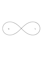
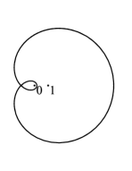
Figure 1. Two shortest non-peripheral curves in the twice punctured plane.

The inequality $A_{0}\geq J$ was actually stated in Jenkins’s paper [21], and this lower bound with the correct value of $J$ contradicts his own upper bound $0.00149$, but he calculated the numerical value of $J$ incorrectly to obtain (1.2). Moreover, he did not notice that his method gives $A_{0}=J$. The details of the computation of the (incorrect) upper bound are omitted in Jenkins’s paper. Because of these and other mistakes in [21], we give in section 2 a complete proof of Theorem 1.1. Our argument in section 2 is essentially the same as that of Jenkins; we only correct his mistakes.

Let $\sigma$ be the circle $\{z:|z|=\sqrt{\rho(f)}\}$, with counterclockwise orientation, and let $\gamma_{f}$ be the image of $\sigma$ under $f$. The definition of $F_{0}$ implies that $\gamma_{f}$ is non-peripheral for $f\in F_{0}$. Only this property is used in Goldberg’s theorems and in Theorem 1.1. However, in applications to Problems 1 and 2 above, the numbers of $0$-, $1$- and $\infty$-points of $f$ in the unit disk are prescribed, and nothing is known a priori about the nature of the curve $\gamma_{f}$. This suggests the following definitions.

For distinct, non-zero integers $N_{0}$ and $N_{1}$ we consider the subclass $F_{0}(N_{0},N_{1})$ of $F_{0}$ consisting of those functions for which the indices of the curve $\gamma_{f}$ about $0$ and $1$ are $N_{0}$ and $N_{1}$, respectively. Then we define

$$A_{0}(N_{0},N_{1})=\inf\{\rho(f):f\in F_{0}(N_{0},N_{1})\}.$$

The classes $F_{j}(N_{0},N_{1})$ and the constants $A_{j}(N_{0},N_{1})$, $1\leq j\leq 4$, are defined similarly. Evidently, $A_{j}(N_{0},N_{1})=A_{j}(N_{1},N_{0})$. One can show that

$$A_{0}(N_{0},N_{1})=A_{1}(N_{0},N_{1})=A_{3}(N_{0},N_{1})<A_{2}(N_{0},N_{1})=A_{4}(N_{0},N_{1})$$

in the same way as Goldberg proved (1.1). Thus it again suffices to consider $A_{0}(N_{0},N_{1})$ and $A_{2}(N_{0},N_{1})$.

Note that if $f\in F_{0}(N_{0},N_{1})$, then

$$\frac{1}{f}\in F_{0}(-N_{0},N_{1}-N_{0})\quad\text{and}\quad f(\rho(f)/z)\in F_{0}(-N_{0},-N_{1}).$$

Thus

$$A_{0}(N_{0},N_{1})=A_{0}(-N_{0},N_{1}-N_{0})\quad\text{and}\quad A_{0}(N_{0},N_{1})=A_{0}(-N_{0},-N_{1}).$$

Together with $A_{0}(N_{0},N_{1})=A_{0}(N_{1},N_{0})$ this implies that we may restrict to the case $N_{0}>N_{1}>0$ in our investigation of $A_{j}(N_{0},N_{1})$ not only if $j=2$, but also if $j=0$. Moreover, we have

(1.3) $$A_{0}(N_{0},N_{1})=A_{0}(N_{0},N_{0}-N_{1}).$$

In section 3 we will prove the following result.

Theorem 1.2.

For $N_{0},N_{1}\in\mathbf{N}$ let $N=N_{0}+N_{1}$ and put $N^{*}=N$ when $N$ is odd and $N^{*}=2N-3$ when $N$ is even. Then

$$A_{0}(N_{0},N_{1})\geq\exp\left(-\frac{\pi^{2}}{\cosh^{-1}(N^{*})}\right).$$

This estimate is best possible (i.e., there exist extremal functions) for all $N\geq 3$.

A corollary of Theorem 1.2 is that

(1.4) $$A_{2}(N_{0},N_{1})\geq\exp\left(-\frac{\pi^{2}}{\log(2\max\{N_{0},N_{1}\})}\right).$$

This improves the result of [8] which in our notation says that

$$A_{2}(N_{0},N_{1})\geq\exp\left\{-\left(1+\frac{2}{\pi e}\right)\frac{\pi^{2}}{\log\min\{N_{0},N_{1}\}}\right\}.$$

Our method allows in principle to compute the exact value of $A_{0}(N_{0},N_{1})$ for any given $N_{0},N_{1}$. The algorithm is described in section 3. For $N=3,4,5,$ we obtain $N^{*}=3,5,5$. For $(N_{0},N_{1})=(2,1),(3,1),(3,2)$ we have equality in our estimate for $A_{0}(N_{0},N_{1})$. We obtain $A_{0}(2,1)=A_{0}$ and

$$A_{0}(3,1)=A_{0}(3,2)=\exp\left(-\frac{\pi^{2}}{\log(5+2\sqrt{6})}\right)\approx 0.013968.$$

However, as apparent already from (1.3), the constant $A_{0}(N_{0},N_{1})$ is not a function of the sum $N_{0}+N_{1}$ only, and we have

(1.5) $$A_{0}(4,1)=A_{0}(4,3)=\exp\left(-\frac{\pi^{2}}{\log(7+4\sqrt{3})}\right)\approx 0.023585.$$

Finding the constants $A_{0}(N_{0},N_{1})$ has the following geometric interpretation. Consider the set of all closed curves in ${\Omega}$ with indices $N_{0},N_{1}$ with respect to $0$ and $1$. Find the minimal hyperbolic length of a curve in this class. Some examples of minimal curves can be seen in Figures 1 and 2.

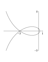
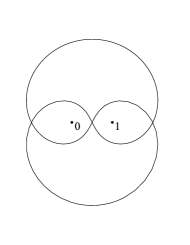
Figure 2. The shortest curve of index $3$ around $0$ and index $2$ around $1$, with magnification of detail, and the shortest curve homotopic to the commutator of the loops around $1$ and $0$.

In section 4 we state a formula for and a conjecture about traces of elements of the principal congruence subgroup $\Gamma(2)$ of the modular group. We found this conjecture while experimenting with traces trying to prove Theorem 1.2, but in our opinion this conjecture is of independent interest.

Goldberg’s theorem says that $A_{2}>A_{0}$, but no explicit estimate of $A_{2}$ from below better than $A_{0}$ was available. Using Theorem 1.2 and a result of Dubinin [13] we can obtain such a bound.

Theorem 1.3.

For every function $f\in F_{2}(N_{0},N_{1})$, we have

(1.6) $$\rho(f)\geq\left(1+\sqrt{1-16A_{0}(N_{0},N_{1})^{2q}}\right)^{2/q}A_{0}(N_{0},N_{1}),$$

where $q$ is the cardinality of $f^{-1}(\{0,1\})$. Moreover,

(1.7) $$A_{2}\geq\left(1+\sqrt{1-16A_{0}^{6}}\right)^{2/3}A_{0}\approx 0.00587465.$$

Now we describe the conjectured extremal function for $A_{2}$. A function $f\in F_{2}$ can be considered as a holomorphic map

(1.8) $$f:\mathbf{U}\backslash f^{-1}(\{0,1\})\to\mathbf{C}\backslash\{0,1\}.$$

Choose a point $z_{0}\in\mathbf{U}\backslash f^{-1}(\{0,1\})$ and let $w_{0}=f(z_{0})$. Then $f$ defines a homomorphism $f_{*}$ of the fundamental groups:

$$f_{*}:\pi(z_{0},\mathbf{U}\backslash f^{-1}(\{0,1\}))\to\pi(w_{0},\mathbf{C}\backslash\{0,1\}).$$

The fundamental group $\pi(w_{0},{\Omega}),$ where ${\Omega}=\mathbf{C}\backslash\{0,1\},$ is a free group on two generators $A$ and $B$ which are simple counterclockwise loops around $0$ and $1$.

The image of the homomorphism $f_{*}$ is a subgroup of $\pi(w_{0},{\Omega})$ which we denote by $\Gamma(f)$. If we change $z_{0}$ and $w_{0}$ we obtain a conjugate subgroup. If (1.8) is a covering map, then $f_{*}$ is injective, so $\Gamma(f)$ is isomorphic to $\pi(z_{0},\mathbf{U}\backslash f^{-1}(\{0,1\}))$; cf. [2, Section 9.4]. We call those functions $f$ for which (1.8) is a covering map locally extremal.

In sections 6 and 7 we define a holomorphic function $h$ in the unit disk, real on $(-1,1)$, with the following properties:

1. $h$ has one double zero at the point $-\mu<0$, and no other zeros,

2. $h$ has one simple $1$-point at the point $\mu$, and no other $1$-points,

3. $h^{\prime}(z)\neq 0$ for $|z|<1,\;z\neq-\mu$,

4. $0,1,\infty$ are the only asymptotic values of $h$, and

5. $\Gamma(h)$ is generated by $A^{2}$ and $B$.

In other words,

$$h:\mathbf{U}\backslash\{-\mu,\mu\}\to\mathbf{C}\backslash\{0,1\}$$

is a covering map corresponding to the subgroup $\langle A^{2},B\rangle$ generated by $A^{2}$ and $B$. This map extends to a function in $\mathbf{U}$ with a double zero at $-\mu$ and a simple $1$-point at $\mu$. We will show that $h$ exists and is uniquely defined by the properties (a)–(e). In particular, $\mu$ is an absolute constant. Actually for a real function in the unit disk, properties (a)–(d) imply (e), but we do not need this fact.

A function $h_{0}$ with a simple root at $0$, no other zeros and no $1$-points in the unit disk, and such that $h_{0}:\mathbf{U}\backslash\{0\}\to{\Omega}$ is a covering map, was studied by Hurwitz [18] and Nehari [24]. These authors found several extremal properties of this function. Our function $h$ and other locally extremal functions introduced in section 6 can be considered as generalizations of this function of Hurwitz.

Evidently, $A_{2}\leq\mu$, so we obtain an upper estimate for $A_{2}$. In section 8 we describe an algorithm to compute $\mu$ with any given precision, and obtain the numerical value:

Theorem 1.4.

$A_{2}\leq\mu\approx 0.0252896$.

In section 9 we study an analytic representation of our function $h$ and describe an algorithm which permits to compute it. We represent $h$ as a composition of the modular function, an elliptic integral and a special solution of the Lamé differential equation.

We conjecture that $A_{2}=\mu$. As supporting evidence we prove the following extremal property of $h$. Let $F_{5}(m,n)$ be the subclass of $F_{2}(m,n)$ consisting of functions having one zero of multiplicity $m$ and one $1$-point of multiplicity $n\neq m$ and put

$$A_{5}(m,n)=\inf\{\rho(f):f\in F_{5}(m,n)\}\quad\text{and}\quad A_{5}=\inf_{m\neq n}A_{5}(m,n).$$

Evidently $A_{5}(m,n)=A_{5}(n,m)$, so it is enough to consider the case $m>n$.

Theorem 1.5.

Let $1\leq n<m$ and $f\in F_{5}(m,n)$. Then $\rho(f)\geq\rho(h)=\mu,$ with equality only for $f(z)=h(e^{i\theta}z)$ with $\theta\in\mathbf{R}$. In particular, $A_{5}=A_{5}(2,1)=\mu$.

We will prove Theorem 1.5 in section 5.

In section 6 we will actually prove a stronger result. We show that every function $f\in F_{5}(m,n)$ is subordinate to some locally extremal function $g$. Subordination means that $f=g\circ\omega$, where $\omega$ is a holomorphic map of $\mathbf{U}$ into itself. So $\rho(f)\geq\rho(g)$ is a consequence of the Schwarz Lemma.

This approach yields functions $h_{m,n}\in F_{5}(m,n)$ which are extremal for $A_{5}(m,n)$. These extremal functions $h_{m,n}$ are defined as covering maps

$$h_{m,n}:\mathbf{U}\backslash\{-\mu_{m,n},\mu_{m,n}\}\to\mathbf{C}\backslash\{0,1\},$$

where $\mu_{m,n}>0$ and $\Gamma(h_{m,n})$ is the group generated by $A^{m}$ and $B^{n}$. The function $h_{m,n}$ is holomorphic in $\mathbf{U}$, has a zero of multiplicity $m$ at $-\mu_{m,n}$ and a $1$-point of multiplicity $n$ at $\mu_{m,n}$. We obtain $A_{5}(m,n)=\mu_{m,n}$ and, up to rotations, $h_{m,n}$ is the unique extremal function $A_{5}(m,n)$.

The computation of the constants $\mu_{m,n}$ is performed with the same method as our computation of $\mu=\mu_{2,1}=A_{5}(2,1)$. Here are some numerical values:

$$\begin{array}[]{l}A_{5}(2,1)=0.0252896,\\ A_{5}(3,1)=0.0849241,\\ A_{5}(4,1)=0.140571,\\ A_{5}(3,2)=0.227417,\\ A_{5}(4,3)=0.290697.\end{array}$$

Theorem 1.5 permits to obtain a complete solution of Problem 1 mentioned above in the simplest case of two points.

Theorem 1.6.

Let $a,b\in\mathbf{U}$. There exists a holomorphic function $f\in F_{2}$ with $f^{-1}(\{0,1\})=\{a,b\}$ if and only if

(1.9) $$\frac{|b-a|}{|1-\overline{a}b|}\geq\frac{2\mu}{1+\mu^{2}}\approx 0.050546,$$

where $\mu$ is the constant of Theorem 1.4 computed in section 8. There exists a rational function $f$ with $f^{-1}(\{0,1\})\cap\mathbf{U}=\{a,b\}$ if and only if the inequality $(\ref{ineq})$ is strict. In this case there even exists a polynomial with this property.

The simplest situation which is not covered by Theorem 1.5 is the case when $f\in F_{2}(2,1)$ has one simple zero and two simple $1$-points. Such a function does not have to be subordinate to any locally extremal function, and we could not prove that $\rho(f)\geq\mu$ in this case.

A problem of control theory dealing with functions in $F_{2}(2,1)$ having one simple zero and two simple $1$-points is the so-called Belgian Chocolate Problem. We will give some applications of our results and methods to this problem in section 11.

2. Preliminaries and the exact value of $A_{0}$

For the background of this section we refer to [1, 2], but note that what we call covering is called complete covering there. A ring is a Riemann surface whose fundamental group is isomorphic to $\mathbf{Z}$. Every ring is conformally equivalent to a region of the form

$$\mathcal{A}=\{z:0\leq\rho<|z|<\rho^{\prime}\leq\infty\}.$$

The number

$$\operatorname{mod}(\mathcal{A})=\frac{1}{2\pi}\log\frac{\rho^{\prime}}{\rho}$$

is called the modulus of the ring. If $\operatorname{mod}(\mathcal{A})<\infty$, then the the ring is called non-degenerate. For a non-degenerate ring we can always take $\rho^{\prime}=1$, thus a non-degenerate ring is equivalent to

(2.1) $$\{z:\rho(\mathcal{A})<|z|<1\},\quad\mbox{where}\quad\rho(\mathcal{A})=\exp\left(-2\pi\operatorname{mod}(\mathcal{A})\right).$$

Consider the universal covering from the upper half-plane $\mathbf{H}$ to a non-degenerate ring $\mathcal{A}$. The group of this covering is a cyclic subgroup of $\mathrm{Aut}(\mathbf{H})$ generated by a hyperbolic transformation, which can be taken to be $z\mapsto\lambda z$ for some $\lambda>1$. It is easy to see that

(2.2) $$\rho(\mathcal{A})=\exp\left(-\frac{2\pi^{2}}{\log\lambda}\right).$$

The hyperbolic metric is defined in the upper half-plane by its length element

$$\frac{|dz|}{\operatorname{Im}z}.$$

It descends from $\mathbf{H}$ to $\mathcal{A}$, and there is a shortest hyperbolic geodesic in the class of the generator of the fundamental group. The hyperbolic length of this shortest geodesic is

$$\ell(\mathcal{A})=\int_{i}^{i\lambda}\frac{|dz|}{\operatorname{Im}z}=\log\lambda.$$

Thus for every non-degenerate ring, there exists a shortest closed geodesic. It is easy to see that no shortest geodesic exists for a degenerate ring $\{0<|z|<1\}$, while in the other degenerate ring, $\{z:0<|z|<\infty\}$ there is no hyperbolic metric, so the notion of shortest geodesic is not defined.

Consider now the region ${\Omega}=\mathbf{C}\backslash\{0,1\}$ and fix a point $z_{0}\in{\Omega}$. The fundamental group $\pi(z_{0},{\Omega})$ is a free group on two generators. Let $\Lambda:\mathbf{H}\to{\Omega}$ be the universal covering. The covering group $\Gamma(2)$ is a group of fractional linear transformations isomorphic to the fundamental group $\pi(z_{0},{\Omega})$. So to each element of $\pi(z_{0},{\Omega})$ corresponds a fractional-linear transformation.

The covering $\Lambda$ and the group $\Gamma(2)$ are explicitly constructed as follows: begin with the region

$$G_{0}=\{z:|\operatorname{Re}z|<1,\;|z-1/2|>1/2,\;|z+1/2|>1/2\}.$$

Let $\Lambda$ be the conformal map of the right half of $G_{0}$ onto $\mathbf{H}$ with the boundary correspondence

$$(0,1,\infty)\mapsto(1,\infty,0).$$

We note that usually a different boundary correspondence is used, but the one chosen above turns out to be convenient for our purposes. The map $\Lambda$ extends to $\mathbf{H}$ by reflections and gives the universal covering $\Lambda:\mathbf{H}\to\Omega$. The fractional linear transformations

$$A(z)=z+2\quad\text{and}\quad B(z)=\frac{z}{-2z+1}$$

perform the pairing of the sides of the quadrilateral $G_{0}$. They are free generators of the covering group $\Gamma(2)$.

The generator $A$ corresponds to a simple counterclockwise loop around $0$ in $\Omega$ and $B$ to a simple counterclockwise loop around $1$.

Fractional-linear transformations mapping $\mathbf{H}$ onto itself are represented by $2\times 2$ matrices with real entries and determinant $1$.

With this representation, $\Gamma(2)$ can be identified with the so-called principal congruence subgroup of level $2$, it is the factor group of the group of all $2\times 2$ matrices $M$ with integer elements and determinant $1$ over the subgroup $\{\pm I\}$. It is freely generated by the two matrices which we denote by the same letters as the two loops described above:

(2.3) $$A=\left(\begin{array}[]{cc}1&2\\ 0&1\end{array}\right)\quad\mbox{and}\quad B=\left(\begin{array}[]{rr}1&0\\ -2&1\end{array}\right).$$

Thus to each element $\gamma$ of $\pi(z_{0},{\Omega})$ corresponds a fractional-linear transformation represented by a pair of matrices $\pm M$. The absolute value of the trace $|\operatorname{tr}M|$ depends only on the conjugacy class of $\gamma$ in $\pi(z_{0},{\Omega})$. The conjugacy classes in $\pi(z_{0},{\Omega})$ are called the free homotopy classes.

Parabolic elements of $\Gamma(2)$ correspond to closed curves in ${\Omega}$ which can be deformed to a point, possibly to a puncture. We call these elements peripheral. Their matrices are characterized by the property that $|\operatorname{tr}M|=2$.

So to every non-peripheral closed curve $\gamma$ in ${\Omega}$ we can associate a hyperbolic element $\phi\in\Gamma(2)$, a ring $\mathcal{A}=\mathbf{H}/\langle\phi\rangle$ and a pair of matrices $\pm M$. Then $\ell(\mathcal{A})$ is the hyperbolic length of the shortest curve in the free homotopy class of $\gamma$, and we have the formulas

(2.4) $$\rho(\mathcal{A})=\exp\left(-\frac{\pi^{2}}{\cosh^{-1}\left(|\operatorname{tr}(M)|/2\right)}\right)$$

and

(2.5) $$\ell(\mathcal{A})=2\cosh^{-1}\left(\frac{|\operatorname{tr}(M)|}{2}\right)=2\log\left(\frac{|\operatorname{tr}(M)|}{2}+\sqrt{\frac{\operatorname{tr}^{2}(M)}{4}-1}\right),$$

or

$$|\operatorname{tr}(M)|=2\cosh\left(\frac{\ell(\mathcal{A})}{2}\right)=2\cosh\left(\frac{\pi^{2}}{\log\rho(\mathcal{A})}\right).$$

Lemma 2.1.

The absolute value of the trace of any non-parabolic element of $\Gamma(2)$ is at least $6$.

Indeed, it is well-known and easy to prove that traces of elements of $\Gamma(2)$ have residue $2$ modulo $4$.

Proof of Theorem 1.1.

Let $f:\mathcal{A}\to{\Omega}$ be a holomorphic function in a ring $\mathcal{A}$, let $z\mapsto\lambda z$ be the fractional-linear transformation corresponding to the generator of the fundamental group of $\mathcal{A}$, as in (2.2), and let $\gamma^{\prime}\in\pi({\Omega})$ be the $f_{*}$-image of this generator. By the assumption of the theorem, the element of $\Gamma(2)$ corresponding to $\gamma^{\prime}$ is hyperbolic, so it is conjugate to $z\mapsto\lambda^{\prime}z$ for some $\lambda^{\prime}>1$. Let $\Gamma^{\prime}$ be the group generated by $z\mapsto\lambda^{\prime}z$, and consider the ring $\mathcal{A}^{\prime}=\mathbf{H}/\Gamma^{\prime}$. Then $f$ induces a holomorphic map $\mathcal{A}\to\mathcal{A}^{\prime}$, and we conclude from the Schwarz Lemma that $\ell(\mathcal{A}^{\prime})\leq\ell(\mathcal{A})$, where equality holds if and only if this holomorphic map is an isometry. So $\lambda\geq\lambda^{\prime}$.

Lemma 2.1 says that the trace of the matrix

$$M=\left(\begin{array}[]{cc}\sqrt{\lambda^{\prime}}&0\\ 0&\sqrt{1/\lambda^{\prime}}\end{array}\right)$$

representing $z\mapsto\lambda^{\prime}z$ is at least $6$, which means that $\lambda^{\prime}\geq(3+2\sqrt{2})^{2}$. Combining this with (2.2) or (2.4) we obtain the inequality stated in the theorem.

To construct an extremal function, we take $\phi\in\Gamma(2)$ with $|\operatorname{tr}\phi|=6$, for example, $\phi=A^{2}B$, and consider the ring $\mathbf{H}/\langle\phi\rangle$. If $\psi$ is a conformal map of this ring onto a ring of the form (2.1) then $\Lambda\circ\psi^{-1}$ is the extremal function. ∎

3. Traces of hyperbolic elements of the principal congruence subgroup

In this section we prove Theorem 1.2. It is deduced from (2.4) and Theorem 3.1 below which estimates the trace of an element of $\Gamma(2)$ corresponding to a curve with given index about $0$ and $1$.

Consider a finite set, which we call an alphabet. A cyclic word is a cyclically ordered finite sequence of the elements of the alphabet. It is helpful to imagine a cyclic word as an inscription on the surface of a cylindrical bracelet. Our alphabet consists of four letters

$$A,B,A^{-1},B^{-1},$$

where $A$ and $A^{-1}$ never occur next to each other, and the same about $B$. We use the usual abbreviation $A^{m}=A\ldots A$ for $m>0$ and $A^{m}=A^{-1}\ldots A^{-1}$ for $m<0$. When writing in a line, a cyclic word can be broken at any place, so every cyclic word distinct from $A^{m}$ and $B^{n}$ can be written as a sequence that begins with some power of $A$ and ends with some power of $B$. If we substitute to such a sequence the free generators of $\Gamma(2)$, $A,B$ as in (2.3), then the trace of the resulting matrix depends only on the cyclic word represented by our sequence, because $\operatorname{tr}(XY)=\operatorname{tr}(YX)$.

So we consider a word

(3.1) $$w=A^{m_{1}}B^{n_{1}}\ldots A^{m_{k}}B^{n_{k}},\quad\mbox{where}\quad|m_{j}|\geq 1,\;|n_{j}|\geq 1,$$

satisfying

(3.2) $$\sum_{j=1}^{k}m_{j}=N_{0},\quad\mbox{and}\quad\sum_{j=1}^{k}n_{j}=N_{1},$$

and estimate $|\operatorname{tr}w|$ from below over all such words. Put

$$\operatorname{length}w=\sum_{j=1}^{k}(|m_{j}|+|n_{j}|).$$

Theorem 3.1.

Let $w$ be a matrix of the form $(\ref{word})$ with $|\operatorname{tr}(w)|\neq 2$. Then

(3.3) $$|\operatorname{tr}w|\geq 2\operatorname{length}w.$$

Moreover

(3.4) $$|\operatorname{tr}w|\geq 4\operatorname{length}w-6\quad\mbox{if}\ \operatorname{length}w\ \mbox{is even}.$$

This estimate is exact as the following words show: $w=A(AB)^{(L-1)/2}$ with $\operatorname{tr}(w)=2L,$ when $L$ is odd, and $w=AB^{L-1},$ with $\operatorname{tr}(w)=4L-6$, when $L$ is even.

Proof of Theorem 1.2.

Let $f\in F_{0}(N_{0},N_{1})$. We proceed as in the proof of Theorem 1.1. With $\mathcal{A}$ and $\gamma^{\prime}$ as defined there we have $\rho(f)=\rho(\mathcal{A})$ and the word $w$ associated to the element of $\Gamma(2)$ corresponding to $\gamma^{\prime}$ satisfies (3.1) and (3.2). The conclusion now follows from (2.4) and Theorem 3.1. ∎

Another result estimating the trace from below is the following theorem which is a special case of a result of Baribaud [4].

Theorem A.

Suppose that a closed geodesic $\gamma$ in $\mathbf{C}\backslash\{0,1\}$ intersects the real line $2n$ times. Then the trace of the element of $\Gamma(2)$ corresponding to this geodesic is at least $2n-2$.

If $f\in F_{0}(N_{0},N_{1})$, then $\gamma_{f}$ intersects the interval $(-\infty,0)$ at least $N_{0}$ times, $(0,1)$ at least $|N_{0}-N_{1}|$ times and $(1,\infty)$ at least $N_{1}$ times. Thus $\gamma_{f}$ intersects the real line at least $n$ times, where $n=N_{0}+N_{1}+|N_{0}-N_{1}|=2\max\{N_{0},N_{1}\}$. Theorem A implies that the conclusion of Theorem 1.2 holds with $N^{*}=2\max\{N_{0},N_{1}\}-1$. This improves Theorem 1.2 and (1.4) if $N_{0}+N_{1}$ is odd and $|N_{0}-N_{1}|>1$, but it does not seem to be possible to deduce the conclusion of Theorem 1.2 in the case that $N_{0}+N_{1}$ is even.

An estimate of the trace from below for the elements of the full modular group $\Gamma$ in terms of the word length is given in [15]. It does not seem to imply Theorems 3.1 or A. Unlike the proof in [4], which is geometric, our proof of Theorem 3.1 is purely algebraic, in the same spirit as the proof in [15].

For the proof of Theorem 3.1 we need two lemmas. Let

$$X=\left(\begin{array}[]{cc}a&b\\ c&d\end{array}\right)$$

be a real matrix. We say that $X$ is decreasing if $|a|>|b|>|d|$ and $|a|>|c|>|d|$, and we define

$$\tau(X)=|a|-|b|-|c|+|d|.$$

Lemma 3.1.

Let $X\in\Gamma(2)$ be a decreasing matrix. Then $\tau(X)\geq 0$. If $\tau(X)=0$, then $X$ has the form

$$X=\left(\begin{array}[]{cc}2k+1&\pm 2k\\ \mp 2k&-(2k-1)\end{array}\right)\quad\mbox{or}\quad X=-\left(\begin{array}[]{cc}2k+1&\pm 2k\\ \mp 2k&-(2k-1)\end{array}\right)$$

for some $k\in\mathbf{N}$. In particular, $\tau(X)=0$ implies that $|\operatorname{tr}X|=2$.

Proof.

Put $|a|=|b|+s$ and $|c|=|d|+t$. Then

$$\pm 1=|a|\cdot|d|-|b|\cdot|c|=|d|s-|b|t,$$

and thus $|d|s\geq|b|t-1$. If $s\leq t-1$, we obtain

$$|b|t-1\leq|d|s\leq|d|(t-1)=|d|t-|d|\leq|d|t-1<|b|t-1,$$

a contradiction. Thus $s\geq t$ and hence

$$|a|+|d|=|b|+|c|+s-t\geq|b|+|c|.$$

If we have equality here, then $s=t$, and thus

$$\pm 1=|d|s-|b|t=(|d|-|b|)s.$$

Thus $t=s=1$ and $|b|=|d|+1$. It follows that there exists $k\in\mathbf{N}$ such that $|a|=2k+1$, $|b|=|c|=2k$ and $|d|=2k-1$. Noting that $ad-bc=1$, we see that $a$ and $d$ have opposite signs, and hence $X$ is of the form given in the lemma. ∎

Lemma 3.2.

Let

$$X=\left(\begin{array}[]{cc}a&b\\ c&d\end{array}\right)\in\Gamma(2)$$

be decreasing, $m,n\in\mathbf{Z}\backslash\{0\},$ and let

$$Y=A^{m}B^{n}X=\left(\begin{array}[]{cc}1-4mn&2m\\ -2n&1\end{array}\right)X.$$

Then $Y$ is decreasing,

(3.5) $$\tau(Y)\geq(4|mn|-2|n|-1)\tau(X)\geq\tau(X),$$

and

(3.6) $$|\operatorname{tr}Y|\geq|\operatorname{tr}X|+\tau(X)(|m|+|n|).$$

If in addition $ad>0$, then

(3.7) $$|\operatorname{tr}Y|\geq|\operatorname{tr}X|+(\tau(X)+2)(|m|+|n|).$$

If $ad>0$ and $mn>0$, and the elements of the main diagonal of $Y$ have opposite signs, then

(3.8) $$\tau(Y)\geq\tau(X)+2.$$

If $mn\neq 1$, then

(3.9) $$\tau(Y)\geq 3\tau(X),$$

and if $mn\neq 1$ and $|\operatorname{tr}X|\neq 2$, then

(3.10) $$|\operatorname{tr}Y|\geq 2|\operatorname{tr}X|+(\tau(X)+2)(|m|+|n|).$$

Proof.

Put

$$Y=\left(\begin{array}[]{cc}\alpha&\beta\\ \gamma&\delta\end{array}\right),$$

so that

$$\alpha = (1-4mn)a+2mc,$$

$$\beta = (1-4mn)b+2md,$$

$$\gamma = -2na+c,$$

$$\delta = -2nb+d.$$

We may assume without loss of generality that $a>0$. Put $\mu=|m|$ and $\nu=|n|$. We distinguish two cases.

Case $1$: $mn>0$; that is, $m$ and $n$ have the same sign. Then

$$|\alpha| = -\alpha=(4\mu\nu-1)a-2\mu|c|\operatorname{sgn}(mc),$$

$$|\beta| = (4\mu\nu-1)|b|-2\mu|d|\operatorname{sgn}(mbd),$$

$$|\gamma| = 2\nu a-|c|\operatorname{sgn}(nc),$$

$$|\delta| = 2\nu b-|d|\operatorname{sgn}(nbd).$$

If $d<0$, then $b$ and $c$ must have opposite signs since $a>0$ and $ad-bc=1$. Since $m$ and $n$ have the same sign by assumption, we obtain

(3.11) $$\operatorname{sgn}(mc)=\operatorname{sgn}(nc)=\operatorname{sgn}(nbd)=\operatorname{sgn}(mbd).$$

If $d>0$, then $b$ and $c$ have the same sign. Again we conclude that (3.11) holds. With $\varepsilon=\operatorname{sgn}(mc)$ we then find in both cases that

$$|\alpha| = (4\mu\nu-1)a-2\varepsilon\mu|c|,$$

$$|\beta| = (4\mu\nu-1)|b|-2\varepsilon\mu|d|,$$

$$|\gamma| = 2\nu a-\varepsilon|c|,$$

$$|\delta| = 2\nu b-\varepsilon|d|.$$

Noting that, by Lemma 3.1,

$$a-|b|=|c|-|d|+\tau(X)\geq|c|-|d|,$$

we find that

$$|\alpha|-|\beta| = (4\mu\nu-1)(a-|b|)-2\varepsilon\mu(|c|-|d|)$$

$$\geq (4\mu\nu-1-2\varepsilon\mu)(|c|-|d|)$$

$$\geq 4\mu\nu-1-2\mu\geq 1,$$

and

$$|\gamma|-|\delta|=2\nu(a-|b|)-\varepsilon(|c|-|d|)\geq(2\nu-\varepsilon)(|c|-|d|)\geq 2\nu-1\geq 1.$$

Since $4\mu\nu\geq 2\mu+2\nu$, we also have

$$|\alpha|-|\gamma|=(4\mu\nu-1-2\nu)a-\varepsilon(2\mu-1)|c|\geq(2\mu-1)(a-|c|)\geq 1,$$

and analogously

$$|\beta|-|\gamma|\geq(4\mu\nu-1-2\nu)|b|-\varepsilon(2\mu-1)|d|\geq 1.$$

Thus $Y$ is decreasing.

Moreover,

$$\tau(Y) = |\alpha|-|\beta|-(|\gamma|-|\delta|)$$

$$= (4\mu\nu-1-2\nu)(a+|b|)-\varepsilon(2\mu-1)(|c|-|d|)$$

$$= (4\mu\nu-1-2\nu)\tau(X)$$

$$+(4\mu\nu-1-2\nu-\varepsilon(2\mu-1))(|c|-|d|)$$

$$\geq (4\mu\nu-1-2\nu)\tau(X)+(4\mu\nu-2\nu-2\mu)(|c|-|d|)$$

$$\geq (4\mu\nu-1-2\nu)\tau(X)\geq\tau(X).$$

This is (3.5).

Next we show that, under the hypothesis stated in the lemma, this lower bound for $\tau(Y)$ can be improved to (3.8) and (3.9). We first note that if $mn\neq 1$, then $\mu\geq 2$ or $\nu\geq 2$ since $m$ and $n$ have the same sign. Thus (3.9) follows from (3) if $mn\neq 1$.

In order to deal with (3.8) we can assume that $ad>0$ and thus $d>0$. Now (3.11) yields

$$\delta=-2\nu|b|\operatorname{sgn}(nb)+d=-2\nu|b|\varepsilon+d,$$

and since $\alpha<0$, we find that the elements $\alpha$ and $\delta$ of the main diagonal of $Y$ have opposite signs if $\varepsilon=-1$. Assuming that this is the case we deduce from (3) that

$$\tau(Y) \geq (4\mu\nu-1-2\nu)\tau(X)+(4\mu\nu-2-2\nu+2\mu)(|c|-|d|)$$

$$\geq \tau(X)+2(|c|-|d|)\geq\tau(X)+2.$$

This is (3.8). Hence we have proved all claims about $\tau(Y)$ in Case 1.

We now turn to the estimates of $\operatorname{tr}Y$. Here we distinguish two subcases.

Subcase $1.1$: $d<0$. Then $\tau(X)=a-d-|b|-|c|$. Thus

$$-\operatorname{tr}Y = (4mn-1)a-2mc+2nb-d$$

$$\geq (4mn-1)a-d-2\mu|c|-2\nu|b|$$

$$= \operatorname{tr}X+2\tau(X)+4(\mu\nu-1)a-2(\mu-1)|c|-2(\nu-1)|b|$$

$$= \operatorname{tr}X+2\tau(X)+4(\mu-1)(\nu-1)a$$

$$+2(\mu-1)(2a-|c|)+2(\nu-1)(2a-|b|).$$

Now $2a-|c|=\operatorname{tr}X+\tau(X)+|b|,$ and $2a-|b|=\operatorname{tr}(X)+\tau(X)+|c|$. Substituting this and using $4(\mu-1)(\nu-1)a\geq 0$, we obtain

$$-\operatorname{tr}Y \geq (1+2(\mu-1)+2(\nu-1))\operatorname{tr}X+(2+2(\mu-1)+2(\nu-1))\tau(X)$$

$$+2(\mu-1)|b|+2(\nu-1)|c|.$$

Since $|b|\geq 2$ and $|c|\geq 2$, this yields

(3.14) $$|\operatorname{tr}Y|\geq(2\mu+2\nu-3)\operatorname{tr}X+(2\mu+2\nu-2)\tau(X)+4(\mu+\nu-1).$$

Now (3.6) follows since $\mu\geq 1$ and $\nu\geq 1$, and thus $2\mu+2\nu-2\geq\mu+\nu$. Moreover, (3.14) may be written in the form

$$|\operatorname{tr}Y| \geq (2\mu+2\nu-3)\operatorname{tr}X+(\mu+\nu)(\tau(X)+2)$$

$$+(\mu+\nu-2)(\tau(X)+2)-4.$$

By Lemma 3.1, we have $\tau(X)\geq 2$ if $|\operatorname{tr}X|\neq 2$. In $mn\neq 1$ and hence $\mu\geq 2$ or $\nu\geq 2$, we have $(\mu+\nu-2)(\tau(X)+2)\geq\tau(X)+2\geq 4,$ and (3.10) follows.

Subcase $1.2$: $d>0$. Since $ad-bc=1$, we see that $b$ and $c$ have the same sign. Thus $mc$ and $nd$ have the same sign. We may assume that $mc>0$. The case that $mc<0$ is analogous. We have similarly to (3)

$$-\operatorname{tr}Y = (4mn-1)a-2mc+2nb-d$$

$$= (4\mu\nu-1)a-2\mu|c|+2\nu|b|-d$$

$$= \operatorname{tr}X+2\tau(X)+4(\mu\nu-1)a$$

$$-2(\mu-1)|c|+2(\nu-1)|b|+4|b|-4d$$

$$= \operatorname{tr}X+2\tau(X)+4(\mu-1)(\nu-1)a$$

$$+2(\mu-1)(2a-|c|)+2(\nu-1)(2a+|b|)+4(|b|-d)$$

$$\geq \operatorname{tr}X+2\tau(X)+4(\mu-1)(\nu-1)a$$

$$+2(\mu-1)(2a-|c|)+2(\nu-1)(2a-|b|).$$

Now

$$2a-|c|=a+\tau(X)+|b|-d\geq\frac{1}{2}\operatorname{tr}X+\tau(X),$$

and

$$2a+|b|\geq\frac{1}{2}\operatorname{tr}(X)+\tau(X).$$

Substituting this into (3) yields

$$|\operatorname{tr}Y| \geq (1+\mu-1+\nu-1)\operatorname{tr}X+(2+2(\mu-1)+2(\nu-1))(\tau(X)+2)$$

$$\geq (\mu+\nu-1)\operatorname{tr}X+(\mu+\nu)(\tau(X)+2),$$

from which (3.7) follows. In particular, we have (3.6). Moreover, if $mn\neq 1$, then $\mu+\nu-1\geq 2$ and thus (3.10) follows.

Case $2$: $mn<0$; that is, $m$ and $n$ have opposite signs. Putting again $\varepsilon=\operatorname{sgn}(mc)$ we now find that

$$|\alpha| = (4\mu\nu+1)a+2\varepsilon\mu|c|,$$

$$|\beta| = (4\mu\nu+1)|b|+2\varepsilon\mu|d|,$$

$$|\gamma| = 2\nu a+\varepsilon|c|,$$

$$|\delta| = 2\nu b+\varepsilon|d|.$$

The proof that $Y$ is decreasing is analogous to Case 1. As in (3) we find that

$$\tau(Y) = (4\mu\nu+1-2\nu)(a+|b|)+\varepsilon(2\mu-1)(|c|-|d|)$$

$$= (4\mu\nu+1-2\nu)\tau(X)+(4\mu\nu+1-2\nu+\varepsilon(2\mu-1))(|c|-|d|)$$

$$\geq (4\mu\nu+1-2\nu)\tau(X)+(4\mu\nu-2\nu-2\mu+2)(|c|-|d|),$$

from which the claimed lower bounds for $\tau(Y)$ easily follow.

Moreover,

$$\operatorname{tr}Y = (4\mu\nu+1)a+2mc-2nb+d$$

$$\geq \operatorname{tr}X+4\mu\nu a-2\mu|c|-2\nu|b|$$

$$= \operatorname{tr}X+2\tau(X)+4(\mu-1)(\nu-1)a$$

$$+2(\mu-1)(2a-|c|)+2(\nu-1)(2a-|b|)+2(a-|d|).$$

Since $2(a-|d|)\geq 0$, we obtain the same inequalities as in (3) and (3), and the conclusion follows from this as above. ∎

Proof of Theorem 3.1.

If $m_{j}=n_{j}=1$ for all $j\in\{1,\ldots,k\}$ then an easy induction shows that

$$w=(-1)^{k}\left(\begin{array}[]{cc}2k+1&-2k\\ 2k&1-2k\end{array}\right),$$

and if $m_{j}=n_{j}=-1$ for all $j$, then

$$w=(-1)^{k}\left(\begin{array}[]{cc}2k+1&2k\\ -2k&1-2k\end{array}\right).$$

Thus $|\operatorname{tr}w|=2$ in these cases. Hence we may assume that not all $m_{j},n_{j}$ are equal to $1$ and not all of them are equal to $-1$.

Suppose first that there exists $j$ such that $|m_{j}|\neq 1$ or $|n_{j}|\neq 1$. Since the trace of a product does not change under cyclic permutations, we may assume that $|m_{k}|\neq 1$ ot $|n_{k}|\neq 1$. Then

$$|\operatorname{tr}(A^{m_{k}}B^{n_{k}})|=|2-4m_{k}n_{k}|\geq 4|m_{k}n_{k}|-2\geq 2(|m_{k}|+|n_{k}|)\geq 6.$$

Now Lemma 3.1 implies that

$$\tau(A^{m_{k}}B^{n_{k}})\geq 2.$$

It follows now from Lemma 3.2 and (3.6) that

$$|\operatorname{tr}(A^{m_{k-1}}B^{n_{k-1}}A^{m_{k}}B^{n_{k}})| \geq |\operatorname{tr}(A^{m_{k}}B^{n_{k}})|+2(|m_{k-1}|+|n_{k-1}|)$$

$$\geq 2(|m_{k-1}|+|n_{k-1}|)+2(|m_{k}|+|n_{k}|).$$

Now (3.3) follows by induction.

Next we note that

$$|\operatorname{tr}(A^{m_{k}}B^{n_{k}})| = 4|m_{k}n_{k}|-2$$

$$= (2|m_{k}|-2)(2|n_{k}|-2)+4(|m_{k}|+|n_{k}|)-6$$

$$\geq 4(|m_{k}|+|n_{k}|)-6.$$

Thus (3.4) follows from (3.5) and (3.6) by induction, whenever

(3.16) $$\tau(A^{m_{k}}B^{n_{k}})\geq 4.$$

If $|m_{k}|\geq 3$ or $|n_{k}|\geq 3$, then

$$\tau(A^{m_{k}}B^{n_{k}})=4|m_{k}n_{k}|-2|m_{k}|-2|n_{k}|=(2|m_{k}|-1)(2|n_{k}|-1)-1\geq 4,$$

so that (3.16) holds. It is easy to see that (3.16) also holds if $|m_{k}|=|n_{k}|=2$ or if $m_{k}n_{k}=-2$. Thus (3.4) holds in these cases, even if the $\operatorname{length}w$ is odd.

The remaining case, apart from the case that $|m_{j}|=|n_{j}|=1$ for all $j\in\{1,\ldots,k\}$, is the case that $m_{k}n_{k}=2$. Here the hypothesis that the $\operatorname{length}w$ is even implies that there exists $l\in\{1,\ldots,k-1\}$ such that $(m_{l},n_{l})\neq(1,1)$, and $(m_{l},n_{l})\neq(-1,1)$. Lemma 3.2, (3.6) and the previous arguments now imply that

$$|\operatorname{tr}(A^{m_{l+1}}B^{n_{l+1}}\ldots A^{m_{k}}B^{n_{k}})|\geq 2\sum_{j=l+1}^{k}(|m_{j}|+|n_{j}|).$$

Moreover, by Lemma 3.2, (3.9) and (3.10) we obtain

$$\tau(A^{m_{l}}B^{n_{l}}\ldots A^{m_{k}}B^{n_{k}})\geq 3\tau(A^{m_{l+1}}B^{n_{l+1}}\ldots A^{m_{k}}B^{n_{k}})\geq 6,$$

and

$$|\operatorname{tr}(A^{m_{l}}B^{n_{l}}\ldots A^{m_{k}}B^{n_{k}})) \geq 2|\operatorname{tr}(A^{m_{l+1}}B^{n_{l+1}}\ldots A^{m_{k}}B^{n_{k}})|+4(|m_{l}|+|n_{l}|)$$

$$\geq 4\sum_{j=l}^{k}(|m_{j}|+|n_{j}|).$$

Now (3.4), and in fact a stronger inequality, follows from Lemma 3.2, (3.5) and (3.6) by induction.

It remains to consider the case that $|m_{j}|=|n_{j}|=1$ for all $j\in\{1,\ldots,k\}$, but not all $m_{j}$ and $n_{j}$ have the same sign. Using cyclic permutations we may assume that $m_{k-1},n_{k-1},m_{k}$ and $n_{k}$ do not all have the same sign. If $m_{k}=-n_{k}\;(=\pm 1)$, then

$$A^{m_{k}}B^{n_{k}}=A^{\pm 1}B^{\mp 1}=\left(\begin{array}[]{cc}5&\pm 2\\ \pm 2&1\end{array}\right),$$

and thus

$$\operatorname{tr}(A^{m_{k}}B^{n_{k}})=6=4(|m_{k}|+|n_{k}|)-2.$$

If there exists $l\in\{1,\ldots,k-1\}$ such that $m_{l}=-n_{l}\;(=\pm 1),$ the proof can be completed as before. We thus may assume that

$$(m_{j},n_{j})\in\{(1,1),(-1,-1)\}\quad\mbox{for}\quad 1\leq j\leq k-1.$$

Suppose that for each $j$ satisfying $l+1\leq j\leq k$ the two main diagonal elements of

(3.17) $$A^{m_{j+1}}B^{n_{j+1}}\ldots A^{m_{k}}B^{n_{k}}$$

have the same sign (which may depend on $j$). Then by (3.7) and induction

$$\operatorname{tr}(A^{m_{l}}B^{m_{l}}\ldots A^{m_{k}}B^{m_{k}}) \geq \operatorname{tr}(A^{m_{k}}B^{m_{k}})+4\sum_{j=l}^{k-1}(|m_{j}|+|n_{j}|)$$

$$\geq 4\sum_{j=l}^{k}(|m_{j}|+|n_{j}|)-2.$$

If $l=1$, we obtain (3.4). If, however, the main diagonal elements of

$$A^{m_{l+1}}B^{m_{l+1}}\ldots A^{m_{k}}B^{m_{k}}$$

have opposite signs for some $l$, and $l$ is the largest number with this property, then by (3.8) we have

$$\tau(A^{m_{l+1}}B^{m_{l+1}}\ldots A^{m_{k}}B^{m_{k}})\geq\tau(A^{m_{l+2}}B^{m_{l+2}}\ldots A^{m_{k}}B^{m_{k}})+2\geq 4.$$

Now the proof is again completed using (3.5) and (3.6).

The case that $m_{k-1}=-n_{k-1}$ can be reduced to the previous one by cyclic permutation.

Suppose finally that $m_{k}=n_{k}=-m_{k-1}=-n_{k-1}$. Then

$$A^{m_{k-1}}B^{n_{k-1}}A^{m_{k}}B^{n_{k}}=\left(\begin{array}[]{cc}13&\pm 8\\ \pm 8&5\end{array}\right),$$

so that

$$\operatorname{tr}(A^{m_{k-1}}B^{n_{k-1}}A^{m_{k}}B^{n_{k}})=18=4\sum_{j=k-1}^{k}(|m_{j}|+|n_{j}|)+2.$$

The proof is now completed by the same arguments as before, distinguishing the cases whether the elements of the main diagonal of (3.17) have the same sign or not. ∎

The proof of Theorem 3.1 shows that the computation of $A_{0}(N_{0},N_{1})$ is equivalent to minimizing $|\operatorname{tr}(w)|$ among all words $w$ of the form (3.1) which satisfy (3.2), the connection being given by (2.4).

In order to find this minimum fix a word $w_{0}$ satisfying (3.2). There are only finitely many words $w_{1},\dots,w_{n}$ satisfying (3.2) for which $\operatorname{length}(w_{j})\leq|\operatorname{tr}(w_{0})|/2$. By Theorem 3.1 it suffices to check these words. With $T:=\min_{0\leq j\leq n}|\operatorname{tr}(w_{j})|$ we deduce from (2.4) that $A_{0}(N_{0},N_{1})=\exp\left(\pi^{2}/\cosh^{-1}(T/2)\right)$.

4. An exact formula and a conjecture about the traces

This section is not needed for understanding of the rest of the paper; it contains a formula for the traces and a conjecture about them that are of independent interest.

We are looking at the trace of the matrix (3.1) which we denote by

$$\left(\begin{array}[]{cc}a_{1,1}&a_{1,2}\\ a_{2,1}&a_{2,2}\end{array}\right).$$

A formula for this matrix and its trace can be easily proved by induction. We have

$$A^{n}=\left(\begin{array}[]{cc}1&2n\\ 0&1\end{array}\right)\quad\text{and}\quad B^{-n}=\left(\begin{array}[]{cc}1&0\\ 2n&1\end{array}\right).$$

The main diagonal elements $a_{1,1}$ and $a_{2,2}$ of the matrix $A^{m_{1}}B^{-n_{1}}\ldots A^{m_{k}}B^{-n_{k}}$ are given by

$$a_{1,1} = 1+4\sum_{i\leq j}m_{i}n_{j}+16\sum_{i_{1}\leq j_{1}<i_{2}\leq j_{2}}m_{i_{1}}n_{j_{1}}m_{i_{2}}n_{j_{2}}+\ldots$$

$$+4^{\ell}\sum_{i_{1}\leq j_{1}<i_{2}\leq j_{2}<\ldots\leq j_{\ell}}m_{i_{1}}n_{j_{1}}m_{i_{2}}n_{j_{2}}\ldots m_{i_{\ell}}n_{j_{\ell}}+\ldots$$

$$+4^{k}m_{1}n_{1}\ldots m_{k}n_{k}$$

and

$$a_{2,2} = 1+4\sum_{i>j}m_{i}n_{j}+16\sum_{i_{1}>j_{1}\geq i_{2}>j_{2}}m_{i_{1}}n_{j_{1}}m_{i_{2}}n_{j_{2}}+\ldots$$

$$+4^{\ell}\sum_{i_{1}>j_{1}\geq i_{2}>j_{2}\geq\ldots>j_{\ell}}m_{i_{1}}n_{j_{1}}m_{i_{2}}n_{j_{2}}\ldots m_{i_{\ell}}n_{j_{\ell}}+\ldots$$

$$+4^{k-1}n_{1}m_{2}n_{2}\ldots n_{k-1}m_{k}.$$

The trace polynomial $a_{11}+a_{22}$ seems to have the followings remarkable property which we verified for $k\leq 6$ using Maple.

Conjecture.

If we substitute $m_{i}=\pm(1+p_{i})$ and $n_{j}=\pm(1+q_{j})$ with arbitrary combination of signs $\pm$, then we obtain a polynomial in $p_{i},q_{j}$ with coefficients of constant sign. This constant sign is equal to the sign of the monomial $\pm 4^{k}p_{1}q_{1}\ldots p_{k}q_{k}$ of the highest degree $2k$.

The off-diagonal elements of the product are given by

$$a_{1,2} = 2\sum_{j=1}^{k}m_{j}+8\sum_{i_{1}\leq j_{1}<i_{2}}m_{i_{1}}n_{j_{1}}m_{i_{2}}+\ldots$$

$$+2\cdot 4^{\ell}\sum_{i_{1}\leq j_{1}<i_{2}\leq j_{2}<\ldots\leq j_{\ell-1}<i_{\ell}}m_{i_{1}}n_{j_{1}}\ldots m_{i_{\ell}}+\ldots$$

and

$$a_{2,1} = 2\sum_{j=1}^{k}n_{j}+8\sum_{j_{1}<i_{1}\leq j_{2}}n_{j_{1}}m_{i_{1}}n_{j_{2}}+\ldots$$

$$+2\cdot 4^{\ell}\sum_{j_{1}<i_{1}\leq j_{2}<\ldots<i_{\ell-1}\leq j_{\ell}}n_{j_{1}}m_{i_{1}}\ldots n_{j_{\ell}}+\ldots.$$

5. Proofs of Theorems 1.3 and 1.5

In the rest of the paper we discuss $A_{2},A_{5}$ and related constants. The idea is that if $f\in F_{2}$, then we can replace the ring $\{\rho(f)<|z|<1\}$ by a larger domain and obtain a stronger estimate than Theorem 1.2 using the same method.

Proof of Theorem 1.3.

Let $f\in F_{2}(N_{0},N_{1})$ and denote by $q$ the cardinality of $f^{-1}(\{0,1\})$. Consider the union $K$ of the $q$ closed segments from $0$ to the points of $f^{-1}(\{0,1\})$. We proceed as in the proof of Theorems 1.1 and 1.2, but replace the ring $\mathcal{A}=\{z:\rho(f)<|z|<1\}$ considered there by the ring $\mathcal{A}:=\mathbf{U}\backslash K$. The arguments used in these proofs now yield that $\rho(\mathcal{A})\geq A_{0}(N_{0},N_{1})$.

For $r>0$ we denote by $K_{q}(r)$ the union of the $q$ segments from $0$ to $re^{2\pi ij}$, $0\leq j\leq q-1$. A result of Dubinin [13, Lemma 1.4 and Theorem 1.10] implies that $\operatorname{mod}(\mathbf{U}\setminus K)\geq\operatorname{mod}(\mathbf{U}\setminus K_{q}(\rho(f))$. With $r:=\rho(f)$ and $\mathcal{A}_{q}(r)=\mathbf{U}\backslash K_{q}(r)$ we thus have $\rho(\mathcal{A})\leq\rho(\mathcal{A}_{q}(r))$. With $R_{q}(r):=\rho(\mathcal{A}_{q}(r))$ we hence find that

(5.1) $$R_{q}(r)\geq A_{0}(N_{0},N_{1}).$$

Since $z\mapsto z^{q}$ is a covering from $\mathcal{A}_{q}(r)$ onto $\mathcal{A}_{1}(r^{q})$ we see that

$$q\operatorname{mod}\mathcal{A}_{q}(r)=\operatorname{mod}\mathcal{A}_{1}(r^{q}).$$

Using the estimate (see, for example, [23, section II.2.3])

$$\operatorname{mod}\mathcal{A}_{1}(t)\geq\frac{1}{2\pi}\log\frac{\left(1+\sqrt{1-t^{2}}\right)^{2}}{t}$$

we obtain

$$q\operatorname{mod}\mathcal{A}_{q}(r)\geq\frac{1}{2\pi}\log\frac{\left(1+\sqrt{1-r^{2q}}\right)^{2}}{r^{q}}.$$

Using (2.1) we thus find that

$$R_{q}^{q}(r)=\rho(\mathcal{A}_{q}(r))^{q}=\exp(-2\pi q\operatorname{mod}\mathcal{A}_{q}(r))\leq\frac{r^{q}}{\left(1+\sqrt{1-r^{2q}}\right)^{2}}.$$

If $r\leq 2^{2/q}R_{q}(r)$ so that $r^{2q}\leq 16R_{q}^{2q}(r)$, this implies that

(5.2) $$\rho(f)=r\geq R_{q}(r)\left(1+\sqrt{1-16R_{q}^{2q}(r)}\right)^{2/q},$$

and if $r>2^{2/q}R_{q}(r)$, then (5.2) is trivially satisfied. Combining (5.1) and (5.2) we obtain (1.6).

To prove (1.7) we note that Theorem 1.2 and the subsequent remarks imply that if $N_{0}+N_{1}>3$, then

$$A_{2}(N_{0},N_{1})\geq A_{0}(N_{0},N_{1})\geq A_{0}(3,1)\approx 0.013968>0.00587465.$$

Thus it suffices to consider functions $f\in F_{2}(2,1)$. For these functions we have $q\in\{2,3\}$. We insert these values for $q$ and $(N_{0},N_{1})=(2,1)$ into (1.6) and find that the smaller bound is obtained for $q=3$. This yields (1.7). ∎

We derive two corollaries from Theorem 1.3. For $f\in F_{2}$ we considered the curve $\gamma_{f}=f(\{z:|z|=\sqrt{\rho(f)}\})$. To the curve $\gamma_{f}$ corresponds a cyclic word in the alphabet $A,B,A^{-1},B^{-1}$, and we denote this cyclic word by $w(f)$.

Corollary 5.1.

Let $f$ be an extremal function for $A_{2}$. Then the cyclic word $w(f)$ can be one of the following:

(5.3) $$A^{2}B,\quad A^{3}B,\quad A^{4}B,\quad A^{2}BAB,\quad A^{2}BABAB,$$

or a word obtained from one of these by permutation of $A$ and $B$.

Proof.

We know from Goldberg’s result that $A_{2}\leq 0.032$, on the other hand, if $|\operatorname{tr}w(f)|\geq 18$, then by formula (2.4) we have $\rho(f)\geq 0.0327$. So for the extremal function $f$ we must have $|\operatorname{tr}w(f)|\leq 14$. Using Theorem 3.1, one can easily make a complete list of words $w$ with $|\operatorname{tr}w|\leq 14$. Up to cyclic permutation or replacement of $(A,B)$ by $(B,A)$, $(A^{-1},B^{-1})$ or $(B^{-1},A^{-1})$, these words are (5.3). ∎

If we are willing to use the numerical value of $\mu$ from Theorem 1.4 instead of the Goldberg estimate, then Corollary 5.1 can be strengthened:

Corollary 5.2.

(Computer assisted) Let $f$ be an extremal function for $A_{2}$. Then the cyclic word $w(f)$ can be one of the following:

$$A^{2}B,\quad A^{3}B,\quad A^{2}BAB,$$

or a word obtained from one of these by permutation of $A$ and $B$.

Proof.

If $w(f)=A^{4}B$, then $f^{-1}(\{0,1\})$ contains at most $5$ points. Thus Theorem 1.3 and (1.5) give

$$\rho(f)\geq\left(1+\sqrt{1-16A_{0}(4,1)}\right)^{2/5}A_{0}(4,1)>0.0310>\mu\approx 0.252896\geq A_{2},$$

which contradicts our assumption that $f$ is extremal for $A_{2}$.

If $w(f)=A^{2}BABAB$, then $f^{-1}(\{0,1\})$ contains at most $7$ points, and Theorem 1.3 with $A_{0}(4,3)=A_{0}(4,1)\approx 0.0235$ gives $\rho(f)>0.286>\mu\geq A_{2}$, which also contradicts the assumption of extremality of $f$. Thus only three words remain as stated in the corollary. ∎

In the proofs of Theorems 1.1-1.3 we considered the hyperbolic length $\ell(\mathcal{A})$ of the shortest geodesic separating the two boundary components of a ring $\mathcal{A}$. In the following, we shall consider domains of higher multiplicity. For a compact, not necessarily connected subset $K$ of the unit disk $\mathbf{U}$ we denote by $\ell(\mathbf{U}\setminus K)$ the hyperbolic length of the shortest geodesic separating $K$ and $\partial\mathbf{U}$ in $\mathbf{U}\setminus K$.

Note that $h$ is a covering which maps the geodesics separating $\{-\mu,\mu\}$ from $\partial\mathbf{U}$ in $\mathbf{U}\setminus\{-\mu,\mu\}$ to the geodesic in ${\Omega}=\mathbf{C}\setminus\{0,1\}$ which is of class $A^{2}B$. The latter geodesic is shown in Figure 1, right. Its length is $2\log(3+2\sqrt{2})$ by Theorem ${1.1^{\prime}}$ or (2.5). Thus

(5.4) $$\ell(\mathbf{U}\setminus\{-\mu,\mu\})=2\log(3+2\sqrt{2}).$$

Proof of Theorem 1.5.

Let $f\in F_{5}(m,n)$ with $m>n\geq 1$. First we note that $\ell(\mathbf{U}\setminus f^{-1}(\{0,1\}))$ remains unchanged if $f$ is replaced by $f\circ T$ for some $T\in\mathrm{Aut}(\mathbf{U})$, but $\rho(f\circ T)$ is minimal if the zero of $f\circ T$ is the negative of the $1$-point of $f\circ T$. With $r=\rho(f)$ we may thus assume that $f(-r)=0$ and $f(r)=1$. Let $\gamma$ be the geodesic separating $\{-r,r\}$ from $\partial\mathbf{U}$ in $\mathbf{U}\setminus\{-r,r\}$. Then $f(\gamma)$ is an non-peripheral curve in ${\Omega}$. By Theorem $1.1^{\prime}$ the hyperbolic length of $f(\gamma)$ in ${\Omega}$ is at least $2\log(3+2\sqrt{2})$. By the Schwarz Lemma, the hyperbolic length of $\gamma$ in $\mathbf{U}\setminus\{-r,r\}$ has the same lower bound and thus

(5.5) $$\ell(\mathbf{U}\setminus\{-r,r\}\geq 2\log(3+2\sqrt{2}).$$

Next we note that $\ell(\mathbf{U}\setminus\{-t,t\})$ is an increasing function of $t$. In fact, $\mathbf{U}\setminus\{-t,t\}$ is conformally equivalent to $\{z:|z|<s/t\}\setminus\{-s,s\}$ and

$$\{z:|z|<s/t\}\setminus\{-s,s\}\subset\mathbf{U}\setminus\{-s,s\}$$

for $0<s<t<1$. Since the hyperbolic metric increases if the domain decreases, we see conclude that $\ell(\mathbf{U}\setminus\{-s,s\})\leq\ell(\mathbf{U}\setminus\{-t,t\})$ for $0<s<t<1$. From (5.4) and (5.5) we now deduce that $\rho(f)=r\geq\mu$.

If we have equality, then $f$ must be a covering and the hyperbolic length of $f(\gamma)$ in ${\Omega}$ must be equal to $2\log(3+2\sqrt{2})$. This implies that the trace of the word associated to the curve $f(\gamma)$ is equal to $6$. Theorem 3.1, together with the assumption that $m>n$, now yields that this word must be $A^{2}B$. We deduce that $f=h$. ∎

6. Locally extremal functions.

A function $g\in F_{2}$ is called locally extremal if

$$g:\mathbf{U}\backslash g^{-1}(\{0,1\})\to{\Omega}=\mathbf{C}\backslash\{0,1\}$$

is a covering map.

Locally extremal functions are labeled by subgroups

$$\Gamma(g):=g_{*}(\pi(z_{0},\mathbf{U}\backslash g^{-1}(\{0,1\})\subset\Gamma(2).$$

These subgroups are generated by finitely many elements, each of which represents a counterclockwise loop, possibly multiple, around $0$ or $1$. We recall that each subgroup $\Gamma$ of the fundamental group $\pi(w_{0},{\Omega})$ corresponds to a covering $g:(X,x_{0})\to({\Omega},w_{0})$ such that $\Gamma=\Gamma(g)=g_{*}(\pi(x_{0},X))$, where $X$ is a hyperbolic Riemann surface which is unique up to conformal equivalence; see, for example, [2, Section 9.4].

In general, parabolic elements in the fundamental group of a Riemann surface correspond to loops around punctures in the surface. If the fundamental group of a Riemann surface is generated by finitely many parabolic elements, then the Riemann surface is conformally equivalent to the plane with finitely many punctures or a disk with finitely many punctures. The first possibility occurs if and only if the product of the parabolic elements generating the fundamental group is also parabolic.

We are interested in the case that $\Gamma=\langle A^{m},B^{n}\rangle$ where $m,n\in\mathbf{N}$, $m\neq n$. We have $\operatorname{tr}(A^{m}B^{n})=4mn-2\geq 6$ and hence $A^{m}B^{n}$ is not parabolic. Thus we may take $X$ to be the unit disk with two punctures, which we can place at the points $-\mu_{m,n}$ and $\mu_{m,n}$ for some $\mu_{m,n}>0$. This determines $\mu_{m,n}$ uniquely. Moreover, $g$ is defined uniquely up to precomposition by $z\mapsto-z$. The functions $g$ extend to the unit disk, taking the values $0$ and $1$ at the punctures $-\mu_{m,n}$ and $\mu_{m,n}$, and we define $h_{m,n}$ to be the function which takes the value $0$ at $-\mu_{m,n}$. The constant $\mu$ and the function $h$ mentioned in the introduction are given by $\mu=\mu_{2,1}$ and $h=h_{2,1}$.

Theorem 6.1.

Let $f\in A_{5}(m,n)$. Then $f$ is subordinate to $h_{m,n}$.

Proof.

Let $z_{0},z_{1}\in\mathbf{U}$ such that $f(z_{0})=0$ and $f(z_{1})=1$. Choose $z^{*}\in\mathbf{U}\setminus\{z_{0},z_{1}\}$. Then $f(z^{*})\not\in\{0,1\}$. Consider simple loops $\gamma_{j}$ in $\mathbf{U}\backslash\{z_{0},z_{1}\}$, beginning and ending at $z^{*}$ and going once around $z_{j}$ counterclockwise. The images $f(\gamma_{j})$ are curves in ${\Omega}$ which begin and end at $f(z^{*})$. They represent elements $\delta_{0}$ and $\delta_{1}$ of the fundamental group $\pi(f(z^{*}),{\Omega})$ which correspond to $A^{m}$ and $B^{n}$. Indeed, the $\gamma_{j}$ are freely homotopic to small simple loops around $z_{j}$, so the $\delta_{j}$ are freely homotopic to loops of multiplicity $m$ and $n$ around $0$ and $1$.

For some germ $\varphi$ of the inverse function of $h_{m,n}$ we now consider the function $\omega=\varphi\circ f$. As $h_{m,n}:\mathbf{U}\setminus\{-\mu_{m,n},\mu_{m,n}\}\to\Omega$ is a covering, $\varphi$ can be continued analytically along every curve in $\mathbf{U}\backslash\{z_{0},z_{1}\}$. Moreover, it follows from the above consideration that the monodromy around the punctures $z_{0}$ and $z_{1}$ is trivial. Thus $\omega$ extends to a map $\omega:\mathbf{U}\to\mathbf{U}$ with $\omega(z_{0})=-\mu_{m,n}$ and $\omega(z_{1})=\mu_{m,n}$. Clearly, $h_{m,n}\circ\omega=f$. ∎

In the next two sections we compute $\mu=\mu_{2,1}$ numerically.

7. Explicit construction of the coverings

We express the local extremal function corresponding to the subgroup $\langle A^{2},B\rangle$ in terms of special conformal mappings. This function is the extremal function $h=h_{2,1}$ described in the introduction.

Let $\mathbf{H}$ be the upper half-plane and consider the regions (cf. Figure 3)

$$G=\left\{z\in\mathbf{H}:0<\operatorname{Re}z|<2,\left|z-\frac{1}{2}\right|>\frac{1}{2}\right\}$$

and

$$G^{\prime}=\left\{z\in\mathbf{H}:0<\operatorname{Re}z<1,\left|z-\frac{1}{2}\right|>\frac{1}{2}\right\}.$$

Figure 3. The regions $G$ and $G^{\prime}$.

Let $\phi:\mathbf{H}\to G$ and $\Lambda:G^{\prime}\to\mathbf{H}$ be conformal homeomorphisms with the following boundary correspondence:

$$\phi:(-1,1,\infty)\mapsto(1,2,\infty),\quad\Lambda:(0,1,\infty)\mapsto(1,\infty,0).$$

We define

(7.1) $$-a=\phi^{-1}(0)<-1.$$

Then $\Lambda$ extends to the upper half-plane by reflections, so the composition

(7.2) $$\tau=\Lambda\circ\phi$$

is a well defined analytic function in $\mathbf{H}$. Evidently, it omits $0,1,\infty$, and $\tau^{\prime}(z)\neq 0$ in $\mathbf{H}$. Now it is not difficult to check that the boundary values of $\tau$ map the interval $\mathbf{R}\cup\{\infty\}\backslash[-1,1]$ into $\mathbf{R}\cup\{\infty\}$. Hence, by the Schwarz Reflection Principle, $\tau$ is meromorphic in $\mathbf{\overline{C}}\backslash[-1,1]$. It is equally easy to check that $\tau$ has a double zero at $\infty$ and a simple $1$-point at $-a$.

The Joukowski function $J(z)=(z+z^{-1})/2$ maps the unit disk conformally onto $\mathbf{\overline{C}}\backslash[-1,1]$, with $J(0)=\infty$ and $J(q)=-a$, where

(7.3) $$q=-a+\sqrt{a^{2}-1}\in(-1,0).$$

Now we define the real conformal automorphism

(7.4) $$\chi(z)=\frac{z-\mu}{1-\mu z}$$

of the unit disk that sends $(-\mu,\mu)$ to $(q,0)$. We obtain

(7.5) $$\mu=\frac{-1+\sqrt{1-q^{2}}}{q}.$$

Then we define our function

(7.6) $$h=1-\tau\circ J\circ\chi.$$

All properties (a)–(d) of $h$ from the introduction are evident now. These properties determine our function $h$ uniquely.

The union of $G$, its reflection in the imaginary axis and the positive imaginary axis is a fundamental domain of the group generated by $A^{2}$ and $B$: $A$ does the vertical sides pairing, and $B$ pairs the circles. So $\Gamma(h)=\langle A^{2},B\rangle$.

8. Computation of the constant $\mu$

We compute the value $a$ in (7.1) We use the notation from the previous section. The function $\phi$ extends by symmetry to

(8.1) $$\phi:Q_{1}=\mathbf{H}\cup\overline{\mathbf{H}}\cup(-1,1)\to Q_{2}=G\cup\overline{G}\cup(1,2).$$

This can be considered as a conformal map between two quadrilaterals. The first quadrilateral has two vertices at $\infty$ and two at $a$, the second one two vertices at $\infty$ and two at $0$.

Every quadrilateral with a chosen pair of opposite sides can be mapped conformally onto a rectangle, so that the chosen sides go to the vertical sides. Such a map is unique, up to rotation of the rectangle by $\pi$. The preimage of the center of this rectangle will be called the center of the quadrilateral.

The harmonic measure of one vertical side at the center is a conformal invariant of a quadrilateral. Our strategy is to compute the harmonic measure $\omega_{0}$ of the circle $|z-1/2|=1/2$ at the center of the quadrilateral $Q_{2}$ in (8.1) numerically. The harmonic measure of the corresponding side $[-a,-1]$ of the quadrilateral $Q_{1}$ can be explicitly computed in terms of $a$. Comparison of the harmonic measures at the centers will give the value of $a$.

Now we give the details. First we handle $Q_{1}$. The part of the boundary that corresponds to the circle of $\partial Q_{2}$ is the interval $[-a,-1]$. First we map $Q_{1}$ onto the unit disk $\mathbf{U}$ by the composition of the real maps

$$z_{1}=\sqrt{\frac{1+z}{1-z}},\quad\mbox{where}\ \sqrt{w}>0\ \mbox{for}\ w>0,$$

and

$$z_{2}=\frac{z_{1}-1}{z_{1}+1}.$$

The points $-a^{+}$ and $-a^{-}$ on the upper and lower sides of $(-\infty,-1]$ are mapped to

(8.2) $$b=\frac{-1+i\sqrt{a^{2}-1}}{a}\quad\mbox{and}\quad\overline{b},$$

respectively. We have

$$\operatorname{Re}b=-\frac{1}{a}\quad\mbox{and}\quad\operatorname{Im}b=\sqrt{1-\frac{1}{a^{2}}}.$$

The points $\infty^{+}$ and $\infty^{-}$ are mapped to $i$ and $-i$, respectively. It is not difficult to see that there exists a real automorphism $\phi$ of the unit disk $\mathbf{U}$ and $w\in\partial\mathbf{U}$ lying in the first quadrant which realize the following boundary correspondence:

$$\phi:(i,b,\overline{b},-i)\mapsto(w,-\overline{w},-w,\overline{w})=:(w,w_{1},w_{2},w_{3}).$$

Since the cross-ratio is invariant under fractional-linear transformations, we find that

$$\left|\frac{b-i}{b+i}\right|^{2}=\frac{(i-b)(-i-\overline{b})}{(i-\overline{b})(-i-b)}=\frac{(w-w_{1})(w_{3}-w_{2})}{(w-w_{2})(w_{3}-w_{1})}=(\operatorname{Re}w)^{2}.$$

For the harmonic measure $\omega_{0}$ of a “vertical side” at the center which we are searching we thus have

$$\omega_{0}=\frac{1}{\pi}\arccos(\operatorname{Re}w)=\frac{1}{\pi}\arccos\left(\left|\frac{b-i}{b+i}\right|\right).$$

Using (8.2) we obtain

$$\omega_{0}=\frac{1}{\pi}\arccos(a-\sqrt{a^{2}-1}),$$

or, inversely,

(8.3) $$a=J(\cos\pi\omega_{0}).$$

Now we compute the corresponding quantity for $Q_{2}$. Do do this, we map $Q_{2}$ conformally onto a region $Q_{3}$ with double symmetry, namely on the unit disk from which two disks of equal radii $r$ tangent from inside at $\pm 1$ are removed. This mapping is performed by the real fractional linear transformation

(8.4) $$\psi(z)=\frac{\sqrt{2}z-2}{\sqrt{2}z+2}$$

which satisfies

$$\psi(0)=-1,\quad\psi(\infty)=1,\quad\psi(2)=-\psi(1),$$

so that

$$r=\frac{1}{2}(1-\psi(2))=\sqrt{2}-1\approx 0.414214.$$

Now $\omega_{0}$ is the harmonic measure of the circle $|z+1-r|=r$ at the center $0$. This is computed numerically, using the Schwarz Alternating Method [19]. Usually this method is applied to a union of regions, but a proper modification also works for the intersection of regions. (To the best of our knowledge, a closed form formula for the modulus of $Q_{2}$ is not known and probably does not exist).

Let us denote by $L=\{z:|z+1-r|=r\}$ the left small circle and by $R=-L$ the right small circle. Then $Q_{3}$ is the region bounded by the unit circle $\partial\mathbf{U}$ and the circles $L$ and $R$. Thus $Q_{3}=G_{L}\cap G_{R}$, where $G_{L}$ is bounded by $L$ and $\partial\mathbf{U}$ and $G_{R}$ is bounded by $R$ and $\partial\mathbf{U}$.

Now define two sequences $(u_{k})$ and $(v_{k})$ of harmonic functions:

• $u_{0}$ is harmonic in $G_{L}$, equals $1$ on $L$ and $0$ on $\partial\mathbf{U}$,

• $v_{0}$ is harmonic in $G_{R}$, equals $u_{0}$ on $R$, and $0$ on $\partial\mathbf{U}$,

• $u_{1}$ is harmonic in $G_{L}$, equals $v_{0}$ on $L$, and $0$ on $\partial\mathbf{U}$,

and so on. Thus, in general,

• $v_{k}$ is harmonic in $G_{R}$, equals $u_{k}$ on $R$, and zero on $\partial\mathbf{U}$,

• $u_{k+1}$ is harmonic in $G_{L}$, equals $v_{k}$ on $L$ and $0$ on $\partial\mathbf{U}$.

All these functions can be computed using the explicit Poisson formulas which are available for $G_{R}$ and $G_{L}$ (see, for example, [22]).

Now a standard argument shows that the alternating series

$$\omega=u_{0}-v_{0}+u_{1}-v_{1}+u_{2}-v_{2}+\ldots$$

converges uniformly on compact subsets of $G$ and satisfies the boundary conditions $\omega(z)=1$, $z\in L$, and $\omega(z)=0$ on the rest of the boundary. Moreover, this series is alternating, so we have an automatic rigorous error control. The speed of convergence is geometric. The computation gives $\omega_{0}\approx 0.483903$.

Substituting this value in (8.3) gives the value

(8.5) $$a\approx 9.91706\;.$$

Now the value $\mu\approx 0.0252896$ follows from (7.3) and (7.5).

To obtain $6$ significant digits, $20$ iterations of the Schwarz method were used. The computation was performed with Maple 14. Matti Vuorinen, Harri Hakula and Antti Rasila verified this computation with a different algorithm. Our Maple script is available on www.math.purdue.edu/$\sim$eremenko.

9. Computation of the extremal function $h$

The contents of this section is close to the papers [9] and [14], studying conformal maps of circular polygons.

We recall that $h$ is given by the formula (7.6), where $\chi$ is a fractional-linear transformation (7.4), $J$ is the Joukowski function, and $\tau$ is defined in (7.2). For the modular function $\Lambda$, explicit expressions are known (see, for example, [3, 19]) and the constant $\mu$ in (7.4) has been computed in the previous section.

It remains to compute $\phi$ in (7.2). Instead we will compute $\theta:=\psi\circ\phi:\mathbf{H}\to Q^{*}$, where

$$Q^{*}=\{z:|z|<1,\;\operatorname{Im}z>0,\;|z-1+r|>r,\;|z+1-r|>r\},\quad r=\sqrt{2}-1,$$

and $\psi$ is the fractional-linear transformation (8.4). The boundary correspondence of $\theta$ is the following:

$$\theta:(\infty,-a,-1,1)\mapsto(1,-1,-1+2r,1-2r).$$

where $a$ has been defined in (7.1) and numerically computed in (8.5).

According to the general theory of conformal mapping of polygons bounded by arcs of circles (see [19, Section III.7.7]), our function $\theta$ is a solution of the Schwarz differential equation

$$\{\theta,z\}:=\frac{\theta^{\prime\prime\prime}}{\theta^{\prime}}-\frac{3}{2}\left(\frac{\theta^{\prime\prime}}{\theta^{\prime}}\right)^{2}=\frac{3}{4}\frac{z^{2}+1}{(z^{2}-1)^{2}}+\frac{1}{2(z+a)^{2}}+\frac{c_{1}}{z-1}+\frac{c_{-1}}{z+1}+\frac{c_{a}}{z+a}.$$

where $c_{1},c_{-1}$ and $c_{a}$ are the real accessory parameters which satisfy two relations

$$c_{a}+c_{1}+c_{-1}=0\quad\mbox{}\quad ac_{a}+c_{1}+c_{-1}=\frac{3}{4},$$

coming from the condition that the angle corresponding to $\infty$ is zero. Thus

$$c_{a}=\frac{3}{4(a-1)}\quad\mbox{and}\quad c_{1}+c_{-1}=-\frac{3}{4(a-1)}.$$

One real parameter, say $c_{1}$, remains. Any real solution $\theta$ of this equation which satisfies $\theta(0)\in\mathbf{R}$ and $\theta^{\prime}(0)>0$ will map the upper half-plane onto a quadrilateral, with interior angles $(0,0,\pi/2,\pi/2)$ at the images of $(\infty,-a,-1,1)$, and the interval $(-1,1)$ will be mapped on the real line. One has to choose the remaining accessory parameter and normalization of $\theta$, so that the vertices with zero angles are at $-1,1$, and the other two vertices are symmetric with respect to $0$ on the interval $(-1,1)$. Then our choice of $a$ and $r$ in the previous section guarantees that the image of $\phi$ is $Q^{*}$, and the boundary correspondence is correct.

To prove that the remaining accessory parameter with the stated properties indeed exists and to obtain a numerical algorithm that finds it, we perform one additional conformal mapping, to explore the symmetry of the problem.

The Schwarz–Christoffel map

(9.1) $$\varphi(z)=C\int_{-1}^{z}\frac{d\zeta}{\sqrt{(\zeta+a)(1-\zeta^{2})}}-\omega,$$

where $C$ is chosen from the condition that $\varphi(-a)=\pi i-\omega$, that is

$$C^{-1}=-\frac{1}{\pi i}\int_{-a}^{-1}\frac{d\zeta}{\sqrt{(\zeta+a)(1-\zeta^{2})}},$$

and

$$\omega=\frac{C}{2}\int_{-1}^{1}\frac{d\zeta}{\sqrt{(\zeta+a)(1-\zeta^{2})}},$$

maps $\mathbf{H}$ onto the rectangle

$$R^{*}=\{x+iy:-\omega<x<\omega,\;0<y<\pi\}.$$

The function $\sigma=\theta\circ\varphi^{-1}$ maps the rectangle onto our region $Q^{*}$. By symmetry, it also maps the right half $R$ of our rectangle onto the right half $Q$ of $Q^{*}$. It is this map

$$\sigma:R\to Q$$

that we are going to compute; cf. Figure 4. A similar problem was solved in [14].

Figure 4. The conformal map $\sigma:(0,\omega,\omega+\pi i,\pi i)\mapsto(0,1-2r,1,i)$.

Let $\wp$ be the Weierstraß elliptic function with periods $2\omega$ and $2\pi i$. We use the standard notation of the theory of elliptic functions as in [3, 19]. We put

$$P(z)=\frac{1}{4}\left(\wp(z+\omega+i\pi)-e_{2}\right).$$

Then $P$ is real on both real and imaginary axis, in fact it maps our rectangle $R$ onto the lower half-plane. The function $P$ is holomorphic in the closure of $R$, except one point $\omega+\pi i$, where it has a pole of the second order.

Our function $\sigma$ will be the ratio of two linearly independent solutions of the Lamé differential equation

(9.2) $$\frac{d^{2}w}{dz^{2}}+Pw=\lambda w,$$

where $\lambda$ is an accessory parameter to be chosen.

Now we describe the choice of $\lambda$. Consider the differential equation obtained by the change of variable $z=it$:

(9.3) $$\frac{d^{2}w}{dt^{2}}=(P(it)-\lambda)w.$$

Let $\lambda_{0}$ be the smallest eigenvalue of (9.3) with the boundary condition $w^{\prime}(0)=w^{\prime}(\pi)=0$. As $P(z)>0$ for $z\in(0,i\pi)$, we conclude from the Sturm comparison theorem [20, Chapter X] that $\lambda_{0}\geq 0$. Let $\lambda_{2}$ be the smallest eigenvalue of (9.3) with the boundary conditions $w^{\prime}(0)=0$, $w(\pi)=0$. By Sturm’s theory we have $\lambda_{2}>\lambda_{0}$.

Let $c(\lambda,z)$ and $s(\lambda,z)$ be two linearly independent solutions of (9.2) normalized by the condition

$$\left(\begin{array}[]{cc}c(0)&s(0)\\ c^{\prime}(0)&s^{\prime}(0)\end{array}\right)=\left(\begin{array}[]{cc}1&0\\ 0&1\end{array}\right).$$

Then

(9.4) $$cs^{\prime}-c^{\prime}s=1,$$

where the primes stand for differentiation with respect to $z$. By our choice of $\lambda_{0}$ we have

$$c^{\prime}(\lambda_{0},i\pi)s(\lambda_{0},i\pi)=0.$$

Together with (9.4) this gives

(9.5) $$c(\lambda_{0},i\pi)s^{\prime}(\lambda_{0},i\pi)=1.$$

By our choice of $\lambda_{2}$ we have

(9.6) $$c(\lambda_{2},i\pi)s^{\prime}(\lambda_{2}(i\pi)=0.$$

The equations (9.5) and (9.6) imply that there exists $\lambda_{1}\in(\lambda_{0},\lambda_{2})$ such that

(9.7) $$c(\lambda_{1},i\pi)s^{\prime}(\lambda_{1},i\pi)=1/2.$$

This $\lambda_{1}$ is our choice of the accessory parameter in (9.2). We will later see that it is unique. For the numerical computation, we solve equation (9.7) on the interval $(\lambda_{0},\lambda_{2})$ by a simple dissection method.

Now we prove that $\sigma(z)=Ks(z)/c(z),$ with a real constant $K$. From now on $\lambda_{1}$ is fixed, and we don’t write it in the formulas. Combining (9.4) and (9.7) we obtain

(9.8) $$c(i\pi)s^{\prime}(i\pi)+c^{\prime}(i\pi)s(i\pi)=0.$$

The function $f:=s/c$ is locally univalent in $\overline{R}\backslash\{\omega+i\pi\}$ as a solution of the Schwarz equation

$$\frac{f^{\prime\prime\prime}}{f^{\prime}}-\frac{3}{2}\left(\frac{f^{\prime\prime}}{f^{\prime}}\right)^{2}=2(P-\lambda_{1}).$$

The functions $c$ and $s$ are real on $[0,\omega]$, because they satisfy a real differential equation and real initial conditions. For the same reason, $c$ is real and $s$ is purely imaginary on $[0,i\pi]$.

We claim that $c$ has no zeros on the sides $[0,\omega]$ and $[0,i\pi]$. On $[0,i\pi]$ this follows from our choice $\lambda_{1}<\lambda_{2}$. Indeed, Sturm’s theory implies that $c$ cannot have zeros on $[0,i\pi]$ for $\lambda<\lambda_{2}$. On $[0,\omega]$ we notice that $P<0$, and $\lambda_{1}>\lambda_{0}\geq 0$, so the solution $c$ with $c(0)=1$ cannot have zeros on $[0,\omega]$. This proves the claim.

We have $f(0)=0$ and $f$ is increasing near $0$ and locally univalent on $[0,\omega]$, so it maps $[0,\omega]$ on some interval $[0,p]$ bijectively. The same applies to $[0,i\pi]$ which is mapped on some interval $[0,iq]$ bijectively. The image of the vertical side $[\omega,\omega+i\pi]$ of the rectangle $R$ must be an arc of a circle $C_{1}$ perpendicular to the real line. To see this, we consider a pair of linearly independent solutions $u,v$ of (9.2) normalized by

$$\left(\begin{array}[]{cc}u(\omega)&v(\omega)\\ u^{\prime}(\omega)&v^{\prime}(\omega)\end{array}\right)=\left(\begin{array}[]{cc}1&0\\ 0&1\end{array}\right).$$

Then $u$ is real and $v$ is purely imaginary on $[\omega,\omega+i\pi]$, for the same reason that $c,s$ are real and imaginary on the imaginary line, and we have

$$c = c(\omega)u+c^{\prime}(\omega)v,$$

$$s = s(\omega)u+s^{\prime}(\omega)v.$$

It follows that $f=s/c$ maps the side $[\omega,\omega+i\pi]$ injectively into the circle

$$\left\{\frac{s(\omega)+s^{\prime}(\omega)it}{c(\omega)+c^{\prime}(\omega)it}:t\in\mathbf{R}\right\}.$$

As the circle is perpendicular to the real line, its center lies on the real line. It is easy to see that the location of the center is

$$\frac{1}{2}\left(\frac{s(\omega)}{c(\omega)}+\frac{s^{\prime}(\omega)}{c^{\prime}(\omega)}\right).$$

Similarly, $f=s/c$ maps the horizontal side $[i\pi,\omega+i\pi]$ injectively into a circle $C_{2}$ perpendicular to the imaginary line whose center is located at

$$\frac{1}{2}\left(\frac{s(i\pi)}{c(i\pi)}+\frac{s^{\prime}(i\pi)}{c^{\prime}(i\pi)}\right).$$

Now equation (9.8) implies that the center of this circle is at the origin. The two circles must have a common point at $f(\omega+i\pi)$ and they must be tangent at this point, because of the form of the Schwarz equation (9.2) near this point. Thus $f$ maps $R$ onto a quadrilateral bounded by a vertical side $[0,iq]$, a horizontal side $[0,p]$ and two circles, perpendicular to the axes which are tangent at one point. Clearly, this tangent point must be on the real line. As the modulus of the quadrilateral $R$ is the same as the modulus of the quadrilateral $Q$, by our choice of the constants $a,\omega$ and $r$, we conclude that $f(R)$ is similar to $Q$, and it remains to multiply $f$ by a constant factor to obtain the function $\sigma$.

Thus we have represented our extremal function $h$ as a composition of the fractional linear transformations $\chi$ and $\psi$ given in (7.4) and (8.4), the Joukowski function $J$, an elliptic integral $\varphi$ in (9.1), a solution of the Schwarz equation which is the ratio of two solutions of the Lamé equation equation (9.2), and the modular function $\Lambda$.

10. Proof of Theorem 1.6

We begin with the following lemma.

Lemma 10.1.

Let $z_{1},\ldots,z_{k}\in\mathbf{U}$, $m_{1},\ldots,m_{k}\in\mathbf{N}$, $f:\mathbf{U}\to\mathbf{C}$ holomorphic and $\varepsilon>0$. Then there exists a polynomial $P$ satisfying $f^{(m)}(z_{j})=P^{(m)}(z_{j})$ for $1\leq j\leq k$ and $0\leq m\leq m_{j}$ such that $|P(z)-f(z)|<\varepsilon$ for $|z|<1-\varepsilon$.

If, in addition, $\{z_{1},\ldots,z_{k}\}=f^{-1}(S)$ for some $S\subset\mathbf{C}$ and $m_{j}$ is the multiplicity of $f$ at $z_{j}$, then $P$ may be chosen such that $P(z)\notin S$ if $|z|<1-\varepsilon$ and $z\notin\{z_{1},\ldots,z_{k}\}$.

Proof.

There exists a polynomial $Q$ satisfying $f^{(m)}(z_{j})=Q^{(m)}(z_{j})$ for $1\leq j\leq k$ and $0\leq m\leq m_{j}$. Let $R(z)=\prod_{j=1}^{k}(z-z_{j})^{m_{j}}$. Then $(f-Q)/R$ is holomorphic in $\mathbf{U}$ and thus the sequence $(T_{k})$ of Taylor polynomials converges locally uniformly in $\mathbf{U}$ to $(f-Q)/R$. With $P_{k}=T_{k}R+Q$ we find that $(P_{k})$ converges locally uniformly to $f$. Moreover, $P_{k}^{(m)}(z_{j})=Q^{(m)}(z_{j})=f^{(m)}(z_{j})$ for $1\leq j\leq k$ and $0\leq m\leq m_{j}$.

Taking $P=P_{k}$ for sufficiently large $k$ we obtain the first conclusion. The second conclusion follows from Hurwitz’s theorem. ∎

Proof of Theorem 1.6.

The quotient on the left-hand side of (1.9) remains unchanged if $a$ and $b$ are replaced by $\phi(a)$ and $\phi(b)$ for some automorphism $\phi$ of $\mathbf{U}$. Thus we may assume without loss of generality that $-b=a>0$. The necessity of the condition (1.9) now follows from Theorem 1.5. It also follows from Theorem 1.5 that equality cannot hold in (1.9) for a rational function.

Conversely, our function $h$ shows that (1.9) is sufficient for the existence of a holomorphic function $f:\mathbf{U}\to\mathbf{C}$ satisfying $f^{-1}(\{0,1\})=\{a,b\}$, and Lemma 10.1 shows that if we have strict inequality in (1.9), then there even exists a polynomial with this property. ∎

11. The Belgian Chocolate Problem

We consider a question posed by Blondel [7, p. 149f] which is known as the “Belgian Chocolate Problem”. We follow [10] in our formulation of this problem:

Let $a(z)=z^{2}-2\delta z+1$ and $b(z)=z^{2}-1$. For which $\delta\in(0,1)$ do there exist stable (real) polynomials $p$ and $q$ with $\deg(p)\geq\deg(q)$ such that $ap+bq$ is stable?

Here a polynomial is called stable if all its roots are in the left half-plane. It is known that there exists $\delta^{*}$ such that $p$ and $q$ as required exist for $0<\delta<\delta^{*}$ and do not exist for $\delta^{*}\leq\delta<1$.

If $p$ and $q$ are as above, then the rational function $R=bq/(ap+bq)$ satisfies $R(1)=0$ and $R(\delta\pm i\sqrt{1-\delta^{2}})=1$, and all other $0$- and $1$-points and all poles of $R$ are in the left half-plane. Passing from the left half-plane to the unit disk by a fractional linear transformation and using Lemma 10.1 we see that the above problem is equivalent to the following one:

For which $t>0$ does there exist a real holomorphic function $f:\mathbf{U}\to\mathbf{C}$ having a simple zero at $0$, simple $1$-points at $\pm it$, and no other $0$- or $1$-points in $\mathbf{U}$?

We find that there exists $t^{*}$ such that a function $f$ with these properties exists for $t^{*}\leq t<1$ and does not exist for $0<t<t^{*}$. The numbers $t^{*}$ and $\delta^{*}$ are related by

$$t^{*}=\sqrt{\frac{1-\delta^{*}}{1+\delta^{*}}}\quad\text{and}\quad\delta^{*}=\frac{1-{t^{*}}^{2}}{1+{t^{*}}^{2}}.$$

Clearly, we have $t^{*}\geq A_{2}$, and Batra’s [6] estimate $A_{2}\geq 0.0012$ also seems to be the best lower bound for $t^{*}$ obtained previously. Theorem 1.3 yields $t^{*}\geq 0.00587$. We can further improve this bound as follows.

Theorem 11.1.

$t^{*}>0.01450779$.

In terms of $\delta^{*}$ this takes the form $\delta^{*}<0.999579$. The best previously known upper bound was $\delta^{*}<0.99999712$, obtained from Batra’s [6] estimate $t^{*}\geq A_{2}\geq 0.0012$. (The frequently cited [10, 11, 25] upper bound $\delta^{*}<0.9999800002$ seems to come from a computational error using the lower bound $A_{2}\geq 10^{-5}$ given in [8].)

The best known lower bound for $\delta^{*}$ is $\delta^{*}>0.973974$; cf. [11]. In terms of $t^{*}$ this takes the form $t^{*}<0.114825$.

Proof of Theorem 11.1.

Let $f:\mathbf{U}\to\mathbf{C}$ be a holomorphic function satisfying $f(0)=0$ and $f(\pm it)=1$, having no further $0$- or $1$-points in $\mathbf{U}$. Theorem ${1.1^{\prime}}$ and the Schwarz Lemma yield that $\ell(\mathbf{U}\setminus\{0,\pm it\})\geq 2\log(3+2\sqrt{2})$. As $z\mapsto-z^{2}$ is a covering map from $\mathbf{U}\setminus\{0,\pm it\}$ onto $\mathbf{U}\setminus\{0,t^{2}\}$, we have $2\ell(\mathbf{U}\setminus\{0,\pm it\})=\ell(\mathbf{U}\setminus\{0,t^{2}\})$. Thus

(11.1) $$\ell(\mathbf{U}\setminus\{0,t^{2}\})\geq\log(3+2\sqrt{2}).$$

We have $\ell(\mathbf{U}\setminus\{0,t^{2}\})=\ell(\mathbf{U}\setminus\{-s,s\})$ with $a$ and $t$ related by $t^{2}=2s/(1+s^{2})$. Thus

$$\ell(\mathbf{U}\setminus\{-s,s\})\geq\log(3+2\sqrt{2}).$$

The equation $\ell(\mathbf{U}\setminus\{-s_{0},s_{0}\})=\log(3+2\sqrt{2})$ is of the same type as (5.4) and can be solved numerically with the method used in section 8 to compute $\mu$, or the one described in [9, Section 5]. We obtain $s_{0}\approx 0.0001054752$ and this implies that $t^{*}\geq\sqrt{2s_{0}/(1+s_{0}^{2})}>0.01450779$. ∎

Remark.

A slightly weaker lower bound for $t^{*}$ can be obtained without computer assistance. Hempel and Smith [17, inequality (9)] showed that

(11.2) $$\ell(\mathbf{U}\setminus\{0,r\})\leq\frac{2\pi^{2}}{\log\left(16\sqrt{1-r}/r\right)-\pi^{2}\left(4\log\left(16\sqrt{1-r}/r\right)\right)^{-1}}$$

for $0<r<1$. Using (11.1) and (11.2) with $r=t^{2}$ we can then show that $t^{*}>0.0132889$.

Acknowledgment.

We thank Peter Buser who brought [4] to our attention and explained it, Vladimir Dubinin and Alexander Solynin for drawing our attention to [13], Andrei Gabrielov for useful discussions, and Matti Vuorinen, Harri Hakula and Antti Rasila for verification of the numerical computation of section 7 with their own method.

References

- [1] L. V. Ahlfors, Complex analysis, 3rd edition, McGraw-Hill, New York, 1978.
- [2] L. V. Ahlfors, Conformal invariants: topics in geometric function theory, McGraw-Hill, New York, 1973.
- [3] N. I. Akhiezer, Elements of the theory of elliptic functions, AMS, Providence, RI, 1990.
- [4] C. M. Baribaud, Closed geodesics on pairs of pants, Israel J. Math., 109 (1999), 339–347.
- [5] P. Batra, On small circles containing zeros and ones of analytic functions, Complex Variables Theory Appl., 49 (2004), no. 11, 787–791.
- [6] P. Batra, On Goldberg’s constant , Comput. Methods Funct. Theory, 7 (2007), no. 11, 33–41.
- [7] V. Blondel, Simultaneous stabilization of linear systems, Springer, Berlin, 1994.
- [8] V. D. Blondel, R. Rupp and H. S. Shapiro, On zero and one points of analytic functions, Complex Variables Theory Appl., 28 (1995), no. 2, 189–192.
- [9] P. R. Brown and R. M. Porter, Conformal mapping of circular quadrilaterals and Weierstrass elliptic functions, Comput. Methods Funct. Theory, 11 (2011), no. 2, 463–486.
- [10] J. Burke, D. Henrion, A. Lewis and M. Overton, Stabilization via nonsmooth, nonconvex optimization, IEEE Trans. Automat. Control 51 (2006), no. 11, 1760–1769.
- [11] Y. J. Chang and N. V. Sahinidis, Global optimization in stabilizing controller design, J. Global Optim. 38 (2007), no. 4, 509–526.
- [12] E. Chirka, On the propagation of holomorphic motions, Dokl. Akad. Nauk 397 (2004), no. 1, 37–40.
- [13] V. N. Dubinin, Symmetrization in the geometric theory of functions of a complex variable, Russian Math. Surveys 49 (1994), no. 1, 1–79.
- [14] A. Eremenko, On the hyperbolic metric of the complement of a rectangular lattice, preprint, arXiv:1110.2696.
- [15] B. Fine, Trace classes and quadratic forms in the modular group, Canad. Math. Bull., 37 (1994), no. 2, 202–212.
- [16] A. A. Goldberg, On a theorem of Landau’s type, Teor. Funktsiĭ Funkcional. Anal. i Priloz̆en., 17 (1973), 200–206 (Russian).
- [17] J. A. Hempel and S. J. Smith, Hyperbolic lengths of geodesics surrounding two punctures, Proc. Amer. Math. Soc., 103 (1988), no. 2, 513–516.
- [18] A. Hurwitz, Über die Anwendung der elliptischen Modulfunktionen auf einem Satz der allgemeinen Funktionentheorie, Vierteljahrsschrift der Naturforschenden Gesellschaft in Zürich, 49 (1904), 242–253.
- [19] A. Hurwitz and R. Courant, Vorlesungen über allgemeine Funktionentheorie und elliptische Funktionen, Springer, Berlin, 1964.
- [20] E. L. Ince, Ordinary differential equations, Longmans, Green and Co., London, 1926. Reprinted by Dover in 1956.
- [21] J. Jenkins, On a problem of A. A. Goldberg, Ann. Univ. Mariae Curie–Skłodowska Sect. A 36/37 (1982/83), 83–86.
- [22] M. Lawrentjew and B. Schabat, Methoden der komplexen Funktionentheorie, VEB Deutscher Verlag der Wissenschaften, Berlin, 1967.
- [23] O. Lehto and K. Virtanen, Quasikonforme Abbildungen, Springer, Berlin, 1965. English translation: Springer 1973.
- [24] Z. Nehari, The elliptic modular function and a class of analytic functions first considered by Hurwitz, Amer. J. Math., 69 (1947), 70–86.
- [25] V. V. Patel, G. Deodhare, T. Viswanath, Some applications of randomized algorithms for control system design, Automatica, 38 (2002), 2085–-2092.
- [26] P. Schmutz Schaller, The modular torus has maximal length spectrum, Geom. Funct. Anal. 6 (1996), no. 6, 1057–1073.
- [27] Z. Slodkowski, Holomorphic motions and polynomial hulls, Proc. Amer. Math. Soc., 111 (1991), no. 2, 347–355.