Adaptive Finite Element Method Assisted by Stochastic Simulation of Chemical Systems

Abstract

Stochastic models of chemical systems are often analysed by solving the corresponding Fokker-Planck equation which is a drift-diffusion partial differential equation for the probability distribution function. Efficient numerical solution of the Fokker-Planck equation requires adaptive mesh refinements. In this paper, we present a mesh refinement approach which makes use of a stochastic simulation of the underlying chemical system. By observing the stochastic trajectory for a relatively short amount of time, the areas of the state space with non-negligible probability density are identified. By refining the finite element mesh in these areas, and coarsening elsewhere, a suitable mesh is constructed and used for the computation of the probability density.

1 Introduction

Stochastic simulation algorithms (SSAs) have been successfully used in recent years to understand a number of biochemical models [3, 30, 39]. However, a systematic analysis of these models is challenging because of the computational intensity of SSAs. A suitable alternative to stochastic simulation is a solution of the chemical Fokker-Planck equation [25, 18]. Consider a well-mixed system of N chemical species and denote by ${\bf x}=(x_{1},\ldots,x_{N})$ a vector of concentrations of these species. The stationary chemical Fokker-Planck equation is a drift-diffusion partial differential equation (PDE) for an $N$-dimensional probability distribution function $p\equiv p({\mathbf{x}})$ where ${\mathbf{x}}\in\Omega\subset{\mathbb{R}}^{N}$, which can be written in the following form:

$$\mathop{\mbox{div}}\big{[}D({\mathbf{x}})\nabla p({\mathbf{x}})-{\mathbf{v}}({\mathbf{x}})p({\mathbf{x}})\big{]}=0$$ (1)

where $D\equiv D({\mathbf{x}}):\Omega\to{\mathbb{R}}^{N\times N}$ is the diffusion matrix, ${\mathbf{v}}\equiv{\mathbf{v}}({\mathbf{x}}):\Omega\to{\mathbb{R}}^{N}$ is the drift term and $\mathop{\mbox{div}}$ is the divergence operator. There have been several methods developed in the literature to solve (1) for moderately large $N$. They include adaptive finite element methods (FEMs) which are commonly used for $N\leq 3$ [4] and sparse grid approaches which are applicable for larger values of $N$ [40]. Adaptive FEMs can be used to identify a suitable mesh which is refined in crucial regions and not in others. Although these approaches can be used for the chemical Fokker-Planck equation, they do not exploit the fact that its solution is a probability distribution of a stochastic process.

In this paper, we present an adaptive mesh construction which is suitable for the FEM solution of (1) if this equation arises from modelling of stochastic chemical systems. The main idea is to exploit the fact that stochastic trajectories spend a significant amount of time in parts of the state space where the mesh refinement is needed. Since adaptive FEMs are mostly applicable for systems up to $N=3$, we will focus on systems of 3 chemical species. However, the presented methodology can be modified for larger (multiscale) chemical systems provided that they have up to $n\leq 3$ important (slow) variables. In [20, 13], a method for estimation of coefficients of an effective Fokker-Planck equation is presented. This effective equation is of the same form as (1) but it is written in the dimension $n$ which is smaller than a total number $N$ of chemical species. If one has a suitable SSA for simulating the low dimensional slow dynamics [10, 9, 17], the presented mesh refinement can be applied. However, since the main aim of this paper is to present this novel numerical methodology, we will not consider any dimensional reduction and restrict to systems which are directly written in terms of $N=3$ chemical species. In the following paper [12], we will show how this mesh refinement can be used to study bifurcation behaviour of stochastic chemical systems.

The paper is organised as follows. In Section 2, we introduce our notation, the Gillespie SSA and the chemical Fokker-Planck equation. In Section 3, we introduce the standard finite element framework that we will use throughout the paper. We also formulate the problem in its weak form in order to define the problem to be solved. In Section 4, we introduce the stochastic simulation assisted adaptive Finite Element Method (saFEM). In Section 5, we offer some insight into how the algorithmic parameters of the saFEM may be chosen in practise. In Section 6, implementational issues related to the algorithm are addressed. Numerical results concerning convergence of the method are presented in Section 7.

2 Chemical Fokker-Planck Equation

Let us consider a well-mixed system of $N$ chemical species $X_{i}$, $i=1,2,\dots,N$, which are subject to $M$ chemical reactions $R_{k}$, $k=1,2,\dots,M$. The state of the system is described by the state vector ${\mathbf{X}}(t)=[X_{1}(t),X_{2}(t),\dots,X_{N}(t)]$ where $X_{i}(t)$ denotes the number of molecules of the corresponding chemical species. Each chemical reaction is described by its propensity function and the stoichiometric vector [23, 19]. The propensity function $\alpha_{k}({\mathbf{x}})$ is defined in such a way that $\alpha_{k}({\mathbf{x}}){\mbox{d}t}$ is the probability that the $k$-th reaction occurs in the infinitesimally small interval $[t,t+{\mbox{d}t})$ provided that ${\mathbf{X}}(t)={\mathbf{x}}.$ The stoichiometric vector is ${\boldsymbol{\nu}}_{k}=[\nu_{k1},\nu_{k2},\dots,\nu_{kN}]$ where $\nu_{ki}$ is the change in $X_{i}$ during reaction $R_{k}$. Stoichiometric vectors form the corresponding stoichiometric matrix $\nu=(\nu_{ki})_{k,i=1}^{M,N}$.

The time evolution of the state vector ${\mathbf{X}}(t)$ is often simulated by the Gillespie SSA [23] which is described in Table 1.

[1] Calculate propensity functions $\alpha_{k}({\mathbf{X}}(t))$, $k=1,2,\dots,M$. [2] Waiting time $\tau$ till next reaction is given by (2). [3] Choose one $j\in\{1,2,\ldots,M\}$, with probability $\alpha_{j}({\mathbf{X}}(t))/\alpha_{0}({\mathbf{X}}(t))$, and perform reaction $R_{j}$, by adding $\nu_{ji}$ to each $X_{i}(t)$ for all $i=1,2,\dots,N$. [4] Continue with step [1] with time $t=t+\tau$.

Table 1: The pseudo code for the Gillespie SSA.

Given the values of the propensity functions (step [1]), the waiting time to the next reaction is given by:

$$\tau=-\frac{\log\left(u\right)}{\alpha_{0}({\mathbf{X}}(t))},\quad\mbox{where}\quad\alpha_{0}({\mathbf{X}}(t))=\sum_{k=1}^{M}\alpha_{k}({\mathbf{X}}(t)),$$ (2)

and $u$ is a uniformly distributed random number in $(0,1)$. The reaction $R_{j}$ is chosen in step [3] using another uniformly distributed random number.

The stationary probability distribution corresponding to the chemical system can be approximated by solving the chemical Fokker-Planck equation [25]. This equation can be written in the form (1) where the diffusion and drift coefficients are:

$$d_{ij}({\mathbf{x}}) = \frac{1}{2}\sum_{k=1}^{M}\nu_{ki}\nu_{kj}\alpha_{k}({\mathbf{x}}),\qquad i,j=1,2,\dots,N,$$ (3)

$$v_{i}({\mathbf{x}}) = \sum_{k=1}^{M}\nu_{ki}\alpha_{k}({\mathbf{x}})-\sum_{j=1}^{N}\frac{\partial d_{ij}}{\partial x_{j}}({\mathbf{x}}),\qquad i=1,2,\dots,N.$$ (4)

This equation is solved on a bounded domain $\Omega\subset[0,\infty)^{N}$ in which the vast majority of the invariant probability density sits [18]. On the boundary $\partial\Omega$ we introduce the homogeneous Neumann boundary condition:

$$\bigl{[}D({\mathbf{x}})\nabla p({\mathbf{x}})+{\mathbf{v}}({\mathbf{x}})p({\mathbf{x}})\bigr{]}\cdot{\mathbf{n}}({\mathbf{x}})=0,\qquad\qquad\rm{for}\ {\mathbf{x}}\in\partial\Omega,$$ (5)

where ${\mathbf{n}}({\mathbf{x}})$ is the outward facing normal at ${\mathbf{x}}\in\partial\Omega$. We seek a solution of (1) which corresponds to the probability distribution function. Therefore, we impose the following normalisation condition:

$$\int_{\Omega}p({\mathbf{x}})\,\mbox{d}{\mathbf{x}}=1.$$ (6)

The choice of the computational domain $\Omega$ might be problematic if we have no a priori information about the problem (1) with (5) and (6). In this case, the stochastic simulations provide a reliable tool to determine the correct $\Omega$ as we will show in Section 4.2. However, before discussing the details of saFEM, we have to introduce some finite element terminology. This will be done in the next section.

3 Finite Element Method

Equation (1) with boundary condition (5) can be numerically solved by the FEM. Since the finite element formulation is based on the corresponding weak formulation, we first introduce the weak solution $p\in H^{1}(\Omega)$ by the equality

$$a(p,\phi)=0,\qquad\qquad\forall\phi\in H^{1}(\Omega).$$ (7)

The bilinear form $a(\cdot,\cdot)$ is naturally given by

$$a(p,\phi)=\int_{\Omega}(D({\mathbf{x}})\nabla p({\mathbf{x}})+p({\mathbf{x}}){\mathbf{v}}({\mathbf{x}}))\cdot\nabla\phi({\mathbf{x}})\,\mbox{d}{\mathbf{x}}.$$ (8)

The finite element formulation is obtained by projecting the weak formulation (7) into a finite dimensional subspace $V_{h}$ of $H^{1}(\Omega)$. Thus, we seek $p_{h}\in V_{h}$ such that

$$a(p_{h},\phi_{h})=0,\qquad\qquad\forall\phi_{h}\in V_{h}.$$ (9)

We note that taking a basis $\phi_{1},\phi_{2},\dots,\phi_{m}$ of $V_{h}$, we can express the finite element solution as

$$p_{h}({\mathbf{x}})=\sum\limits_{i=1}^{m}p^{i}\phi_{i}({\mathbf{x}}),\quad{\mathbf{x}}\in\Omega.$$

Here, the coefficients $p^{i}\in{\mathbb{R}}$ solve the system of linear algebraic equations

$$A{\mathbf{p}}=0,$$ (10)

where ${\mathbf{p}}=(p^{1},p^{2},\dots,p^{m})^{T}$ and the stiffness matrix $A\in{\mathbb{R}}^{m\times m}$ is defined by its entries

$$A_{ij}=a(\phi_{j},\phi_{i}),\quad i,j=1,2,\dots,m.$$ (11)

We construct the finite element space $V_{h}$ and the corresponding basis functions in the standard way [11]. In what follows, we will focus on computations in three dimensions, i.e. $N=3$. We consider the finite element mesh ${\mathcal{T}}_{h}$ consisting of tetrahedral elements. The lowest-order finite element space $V_{h}$ then consists of globally continuous and piecewise linear functions over the mesh ${\mathcal{T}}_{h}$:

$$V_{h}=\{\phi_{h}\in H^{1}(\Omega):\phi_{h}|_{K}\in\mathbb{P}^{1}(K)\mbox{ for all }K\in{\mathcal{T}}_{h}\},$$ (12)

where $\mathbb{P}^{1}(K)$ stands for the space of linear functions over the tetrahedron $K\in{\mathcal{T}}_{h}$. If ${\mathbf{q}}_{j}\in{\mathbb{R}}^{3}$, $j=1,2,\dots,m$, stand for the nodes of the mesh ${\mathcal{T}}_{h}$ then the standard finite element basis functions $\phi_{i}$ are uniquely determined by the condition

$$\phi_{i}({\mathbf{q}}_{j})=\delta_{ij},\quad i,j=1,2,\dots,m,$$

where $\delta_{ij}$ stands for Kronecker’s symbol.

An efficient solution to problem (9) can be obtained by employing adaptively refined meshes [38]. The optimally adapted mesh leads to an approximation with the smallest error, provided the number of degrees of freedom is fixed. Practically, the optimal mesh can be hard to determine, but meshes close to the optimal can be found. These meshes are fine in regions where the solution exhibits steep gradients, boundary layers, interior layers or singularities, and they are relatively coarse in the other regions.

The standard numerical approach for construction of nearly optimal meshes is the adaptive algorithm based on suitable a posteriori error estimators [4, 38]. This algorithm starts with an initial coarse mesh and refines it adaptively by a sequence of refinement steps. In each step, problem (9) has to be solved on the actual mesh, an error indicator has to be computed for each element, and based on these indicators the mesh is refined at suitable places. Using the mesh refinements assisted by stochastic simulations, we can avoid the sequence of refinement steps and construct a suitably adapted mesh at once.

4 Adaptive mesh refinement assisted by stochastic simulations

Since the chemical Fokker-Planck equation (1) is a continuous approximation of the evolution of the probability density given by the Gillespie SSA[23], one can expect that trajectories simulated from the SSA will be informative. Once the trajectory has reached probabilistic equilibrium, regions surrounding the path of the trajectory are likely to be regions with non-negligible invariant density with respect to the steady state Fokker-Planck equation. We should be aiming to refine the finite element mesh in regions where the rate of change of the gradient of the invariant density is larger. The area in which we should be trying to refine our mesh can be well approximated by the region which has non-negligible invariant density. Therefore, stochastic simulations of the chemical system can be informative about a good choice of finite element mesh.

The construction of the locally adapted mesh assisted by stochastic simulations is done in three stages. In Stage I, we use the stochastic simulations to identify those regions of the state space, where the system spends most of its time, and hence where we are interested to resolve the problem with the highest accuracy. In Stage II, we identify the computational domain $\Omega$ as a cuboid that covers the region from Stage I and its neighbourhood. In Stage III, we construct the actual mesh in the computational domain $\Omega$ based on the information from Stage I. In what follows, we provide detailed description of these three stages in the case of $N=3$ chemical species. Following the notation of Section 2, the chemical species will be denoted as $X_{1}$, $X_{2}$ and $X_{3}$. The mesh generation algorithm is summarised in Table 2.

[1] Identify steady states (stable and unstable) of the mean field approximation of the system, or in the case of oscillatory systems, one (or more) coordinates along the limit cycle. We denote these $S\in\mathbb{N}$ points by $\{{\mathbf{y}}_{k}\}_{k=1}^{S}$. [2] Run one (or more) Gillespie simulations of length $B+T>0$ for each of the initial conditions $\{{\mathbf{y}}_{k}\}_{k=1}^{S}$. Here, $B\geq 0$ is the length of a possible initial transient and $T>0$. Take a subsample of $Q>0$ points per unit time per trajectory in the time interval $[B,B+T]$ and denote them as in (14). We also denote by $x_{i}^{\rm max}$ (resp. $x_{i}^{\rm min}$) the maximal (resp. minimal) value of the $i$-th chemical species, $i=1,2,3$, during time intervals $[B,B+T]$ of all $S$ simulations. [3] Use (15), to define a neighbourhood $\Gamma\subset[0,\infty)^{N}$ of the points (14) as the region of the domain in which we require the finest level of refinement of the mesh. This is made up of ellipsoids around each point with radii given by (17) with parameter $\beta_{1}>0.$ [4] Define the domain of solution $\Omega$ by (18), using parameter $\beta_{2}>0.$ [5] Start with the mesh as one single cuboid covering the whole of $\Omega$. [6] Loop over all cuboids in the mesh. If the cuboid is sufficiently close (as given by (19)) to $\Gamma$, then split the cuboid into eight equally sized cuboids. Update the list of hanging nodes/hang type (face/edge hanging node as shown in Figure 2 (left)). [7] Repeat step [6] until the maximum resolution has been reached after $H\in\mathbb{N}$ iterations, or the maximum total number of cuboids has been reached.

Table 2: Mesh generation using SSA trajectories.

4.1 Stage I: Stochastic simulation

In step [1] of Table 2, we identify structures that a priori should exist in the probability density. An indication of the regions which may contain significant amounts of invariant density can be found by analysing the 3-dimensional system of ordinary differential equations (ODEs)

$$\frac{\mbox{d}x_{i}}{{\mbox{d}t}}=v_{i}(x_{1},x_{2},x_{3}),\qquad i\in\{1,2,3\},$$ (13)

which is closely related the mean field approximation of the chemical system. Steady states of ODE system (13) will often coincide with regions of the solution of the steady state Fokker-Planck equation (1) that have large density. The most important things to identify are stable steady states of (13), which can be found by solving an algebraic system $[v_{1}(x_{1},x_{2},x_{3}),v_{2}(x_{1},x_{2},x_{3}),v_{3}(x_{1},x_{2},x_{3})]=0$. In oscillating systems, one can identify limit cycles. There are several tools in the literature for analysis of ODEs of the form (13), such as AUTO [15].

In step [2], these steady states can then be used as starting points for SSA trajectories, once the numbers of molecules of each species have been rounded to the nearest integer. One might additionally wish to ensure that each chain is starting in probabilistic equilibrium by running a short simulation of length $B\geq 0$ from these points before starting the sampling procedure. The Gillespie SSA is detailed in Table 1. In the case of limit cycles, several points along the limit cycle can be used as starting points for the SSA. Either way, we denote the $S$ starting positions for the trajectories by $\{{\mathbf{y}}_{k}\}_{k=1}^{S}\subset{\mathbb{R}}^{3}$. The trajectories simulated up to some time $B+T>0$ using the SSA can help inform us about the regions of domain which will have non-negligible invariant density. Since the trajectories will contain many points, we cannot store all of the points that are simulated. Instead, we subsample from the trajectories at equidistant time points, at a rate $Q>0$ points per unit time. This leaves us with a set of sampled points

$$\left\{{\mathbf{z}}_{k,l}\right\}_{k=1,l=1}^{S,\lfloor QT\rfloor}\subset{\mathbb{R}}^{3}$$ (14)

from the invariant distribution, where $\lfloor QT\rfloor$ denotes the integer part of the real number $QT$. We hope to recover, from this set of points (14), information about what might be an optimal finite element mesh. We also denote by $x_{i}^{\rm max}$ (resp. $x_{i}^{\rm min}$) the maximal (resp. minimal) value of the $i$-th chemical species, $i=1,2,3$, during time intervals $[B,B+T]$ of all $S$ simulations. These numbers will be useful in (16)–(17). In step [3], we make the approximation that the region which contains the majority of the invariant density, is a subset of the union of a set of ellipsoids centred at each point (14), namely

$$\Gamma\equiv\bigcup_{k,l}\mathcal{E}_{{\mathbf{r}}}({\mathbf{z}}_{k,l}).$$ (15)

Here, $\mathcal{E}_{{\mathbf{r}}}({\mathbf{z}}_{k,l})$ is an ellipsoid with radii ${{\mathbf{r}}}=[r_{1},r_{2},r_{3}]$ centred at point ${\mathbf{z}}_{k,l}$ for $k=1,2,\dots,S,$ $l=1,2,\dots,\lfloor QT\rfloor$. These radii can be picked to be proportional to the range of each chemical species using the parameter $\beta_{1}>0$ and numbers $x_{i}^{\rm min}$, $x_{i}^{\rm max}$, $i=1,2,3$, computed in step [2]. Namely, we define

$$x_{i}^{\rm range}=x_{i}^{\rm max}-x_{i}^{\rm min},\qquad\qquad i=1,2,3,$$ (16)

and

$${\bf r}=\beta_{1}\left(x_{1}^{\rm range},\,x_{2}^{\rm range},\,x_{3}^{\rm range}\right).$$ (17)

One should note that the parameters B and T might in principle be different for different initial conditions $y_{k}$, but to simplify the notation, we do not stress this fact by using the notation $B_{k}$ and $T_{k}$ and use simply $B$ and $T$.

4.2 Stage II: Automatic detection of the domain

Next, we would like to identify the domain $\Omega$ on which we wish to solve (1). Since we already have an approximation of the region which contains the majority of the probability density, we can simply fit a cuboid around this region, and then extend it by a factor. The only other condition that we enforce is that the domain must be contained by the positive quadrant of the state space. In step [4], we pick a parameter $\beta_{2}>0$ to define how much we would like to extend the cuboid:

$$\Omega={\mathcal{A}}_{1}\times{\mathcal{A}}_{2}\times{\mathcal{A}}_{3},$$ (18)

where

$${\mathcal{A}}_{i}=\left(\max\{0,x_{i}^{\rm min}-\beta_{2}\,x_{i}^{\rm range}\},x_{i}^{\rm max}+\beta_{2}\,x_{i}^{\rm range}\right),\qquad\qquad i=1,2,3.$$

We then wish to solve (1) on the domain $\Omega$ with boundary conditions (5) on $\partial\Omega$.

4.3 Stage III: Construction of the adaptive mesh

In this stage, we construct the adaptively refined mesh. In the previous stage we naturally defined the computational domain as a cuboid (18). Therefore, we base our refinement approach on simple splitting of a cuboid into 8 congruent sub-cuboids, as shown in Figure 1. However, any other standard mesh refinement technique can be utilised instead.

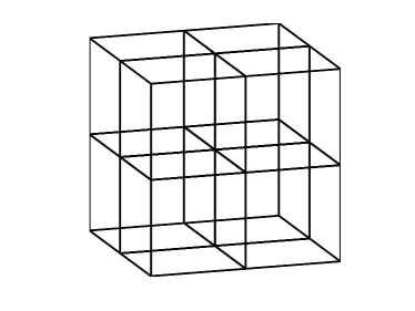
Fig. 1: Example of a single cuboid after the proposed refinement into $8$ sub-cuboids.

An advantage of the refinement of cuboids into 8 sub-cuboids is its simplicity. A disadvantage is that these refinements produce so-called hanging nodes in the mesh, see Figure 2 (left).

In step [5] of the mesh generation, our mesh consists of a single large cuboid. We then, in step [6], iteratively refine cuboids in the following fashion. In each iteration of the refinement procedure, we loop over all of the current cuboids that exist following the previous iteration of the method. For each of the cuboids $I_{1}\times I_{2}\times I_{3}$, where $I_{1},I_{2},I_{3}\subset[0,\infty)$ are intervals, we compute the minimum distance between all points in this cuboid, and the set of points (15) in each coordinate, namely

$$\mbox{dist}(\Gamma,I_{i})=\inf\{|a_{i}-b_{i}|:[a_{1},a_{2},a_{3}]\in\Gamma,\,b_{i}\in I_{i}\},\qquad\qquad i=1,2,3.$$

We refine the given cuboid $I_{1}\times I_{2}\times I_{3}$ if

$$\mbox{dist}(\Gamma,I_{i})<|I_{i}|\qquad\mbox{is satisfied for every}\;i=1,2,3.$$ (19)

If a cuboid is to be refined, it is split into 8 cuboids of equal volume. As detailed in step [7], this refinement condition can be iterated for a set number of times $H\in\mathbb{N}$, where $\mathbb{N}\equiv\{1,2,3,\ldots\}$, or until the number of cuboids present in the mesh is as large as we would like or can deal with given our computational resources.

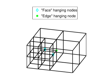
             (a)          (b)

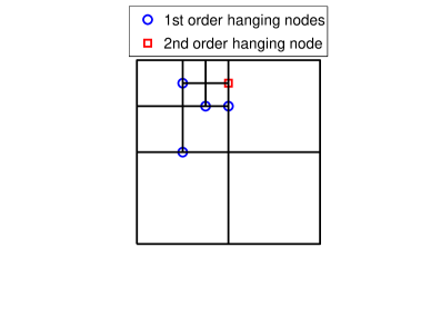
Fig. 2: (a) $1^{st}$ order hanging nodes of different types in cuboid meshes. (b) Hanging nodes of order $1$ and order $2$ on a 2D mesh.

Notice that the algorithm described above produces hanging nodes of order one only. This means that two neighbouring elements in the mesh are either of equal size or one of them has eight times greater volume than the other one. This is important for practical implementation, because the hanging nodes of order one are much easier to work with than the hanging nodes of higher orders. See [37] for more details and Figure 2(b) for an illustration in 2D. In order to guarantee the continuity of the approximation, the value of the function at the hanging node is necessarily decided by the values of the function at the vertices of the less refined cube. Therefore the hanging nodes are not in actual fact additional degrees of freedom in the problem. Thus, the dimension of problem (10) is equal to the total number of vertices in the generated mesh, less the number of hanging nodes. This special treatment of hanging nodes actually enforces on us a mesh which is highly refined in the regions which we wish it to be, and then the mesh becomes gradually coarser as we move away from those regions.

4.4 Tetrahedral mesh

Once the cuboid mesh has been generated by steps [1]–[7] of Table 2, we can then implement a finite element method on it. In the numerics shown in this paper, we further split each cuboid into 6 path tetrahedra. However there is nothing to say that we could not use cubic elements, but we use tetrahedra to simplify some implementational issues.

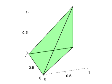
             (a)          (b)

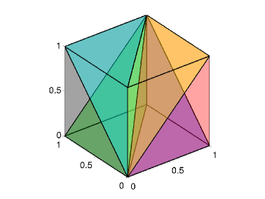
Fig. 3: (a) Example of one element from the refinement scheme. (b) Example of a unit cube split into 6 elements of equal size and shape.

We choose a refinement regime in which the elements are clustered in groups of 6 non-obtuse tetrahedra which together form each cuboid [7]. Figure 3(a) shows an example element from the refinement scheme. The idea is that if we map each cuboid to the unit cube, then each element is exactly of the same shape and size as all the others. Figure 3(b) shows how 6 of these elements can tessellate into a cube.

A lot of refinement methods in the literature involve splitting each element into several smaller elements[31]. However, if this is not done in a clever way, this can lead to degradation of the quality of the elements. That is, some of the angles of the elements may become too small, leading to long thin elements, which can lead to less accuracy in the approximation[8].

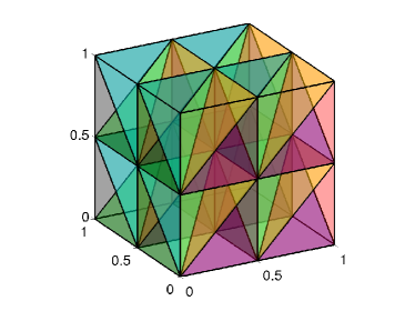
Fig. 4: Example of a unit cube after a refinement iteration.

In the method that we propose here, instead of splitting each element, we split each cuboid into 8 equally sized cuboids. Each cuboid is then split, as before, into 6 equally sized and shaped (after a linear transformation if not a cube) tetrahedral elements. Figure 4 shows a cube which has been refined once and been split into 48 elements, with 27 vertices.

5 Parameter Selection

The algorithm has several parameters $S$, $T$, $Q$, $B$, $\beta_{1}$, $\beta_{2}$ and $H$ whose values must be decided by the user. The parameters $S$, $T$, $Q$, $B$ relate to the implementation of the Gillespie SSA, and the remaining three $\beta_{1}$, $\beta_{2}$, $H$ relate to the selection of the domain and the mesh, given the recorded output of the SSA. In this section we suggest how one might go about selecting values for these parameters.

5.1 SSA parameters

The purpose of simulating the SSA trajectories, as described in Subsection 4.1, is to get an indication of the regions of the domain which contain the majority of the invariant probability density. There are four parameters to consider, $S\in{\mathbb{N}}$, $T>0$, $Q>0$ and $B\geq 0$. The parameter $B$ represents the length of the simulated trajectory that we ignore at the beginning of the simulation. This period of simulation is simply used to ensure that the Markov chain has entered probabilistic equilibrium. This ensures that it is highly likely the point in state space where the rest of the trajectory starts has non-negligible density with respect to the invariant distribution. The final parameter, $Q$, represents the rate (per unit time) at which we record samples from each trajectory in the time interval $[B,B+T]$. This parameter is necessary since if we recorded every single state that the trajectory passed through, we could quickly run out of memory.

Choosing sensible values for these parameters is not easy, since it is problem dependent. However, our aim is not to run such a long trajectory that simply using a histogram of the values would lead to an accurate approximation of the invariant density, as this would completely negate the need for the rest of the algorithm. Likewise, if the trajectory is too short, we will have a very poor approximation of the areas of the domain which contain the majority of the probability density. Our aim, therefore, is to get as good an approximation of this region as possible with the shortest possible trajectories.

As with many Monte Carlo estimates, due to the law of large numbers, the error decays at a rate proportional to $1/\sqrt{T}$. It is reasonable to expect that the approximation of the region which contains the majority of the invariant density should decay at a similar rate. Since convergence diagnostics relating to Markov chains are an open area with no hard and fast solution[14], we suggest that a sample trajectory be created a priori to ascertain the relaxation time of the system. The parameter $B$ can simply be set to be a proportion of the length $T$, for instance $B=T/10$. The parameter $Q$ should be picked according to how much memory one would like to set aside to store the sampled points. Since we are calculating minimum distances to any point in this set in step [6] of the algorithm, the more points there are, the longer the algorithm will take to run.

5.2 Domain and mesh generation parameters

The domain and mesh generation parameters are given by $\beta_{1}>0$, $\beta_{2}>0$ and $H\in\mathbb{N}$. The parameter $\beta_{2}$ defines the size of the domain as seen in (18). Unless the trajectories from the SSA are very short, the estimation of the domain should be relatively trivial, and a value of order 1 should suffice in most instances. The value of $\beta_{1}$, which indicates how much error we estimate there to be in our estimation of the region which contains the majority of the invariant density, should be directly proportional to $1/\sqrt{T}$. Too large a value will lead to unnecessary refinement in some areas, while too small a value will lead to not enough refinement and more error. The parameter $H$ indicates the maximum number of splits that the initial cubes of the mesh may undergo. In practice this can be found at runtime, by capping the total number of elements we allow in the mesh due to memory and CPU constraints.

5.3 A numerical test of accuracy

Although the method has seven parameters which have to be specified, it is relatively easy to check that the computed results are numerically accurate. Given the parameter set $\{S,T,Q,B,\beta_{1},\beta_{2},H\}$, we can compare the computed results with the results obtained with the parameter set $\{S,2T,2Q,2B,2\beta_{1},\beta_{2},H+1\}$. If the result does not change significantly, then we can conclude that our parameters were chosen sufficiently large. Here, the parameters $T$, $Q$, $B$, and $\beta_{1}$, are multiplied by $2$ because increasing any of these parameters will increase the accuracy of the solution. In a similar way $H$ can be increased by one, which means that the finest level of refinement in the mesh becomes smaller by a factor of two in each coordinate. However, we do not propose to modify $S$ and $\beta_{2}$ for the following reasons. The number of starting points $S$ can be determined by the number of stable equilibria of (13). In this case, the parameter $S$ does not have to be changed during this a posteriori test of accuracy. Furthermore, $\beta_{2}$ is used only to choose the size of the domain, and multiplying the size of the domain by $2$ would lead to a smaller proportion of the domain being covered by $\Gamma$ (given by (15)), and as such a more accurate solution would not be guaranteed. If one wishes to test whether $\beta_{2}$ is large enough, the parameter $H$ may have to be increased as a function of $\beta_{2}$ in order to maintain the same level of refinement in $\Gamma$.

6 Implementation of the saFEM

As soon as the computational mesh is determined, the approximation $p_{h}\in V_{h}$ of the invariant distribution $p$ is computed by the standard FEM approach [11, 37]. In order to compute the entries of the stiffness matrix (11), it is necessary to use suitable quadrature routines. In numerical examples below, we consider chemical reactions of at most second order. Therefore, the diffusion $D({\mathbf{x}})$ and drift ${\mathbf{v}}({\mathbf{x}})$ coefficients are polynomials of degree at most two. Since the finite element space consists of piecewise linear functions, it suffices to use a tetrahedral quadrature rule of order three which integrates cubic polynomials exactly. The optimal (Gauss) quadrature rule on tetrahedra of order three has 5 points [37].

Since the dimension of the resulting algebraic system (10) can be very large, even for relatively coarse approximations, parallelisation of the assembly process is of paramount importance. Several packages exist for constructing matrices in parallel. The Portable Extensible Toolkit for Scientific Computation (PETSc) is a suite of data structures and routines for the scalable (parallel) solution of scientific applications modelled by PDEs[6, 5]. The matrix is split into sections which are controlled by each processor. If the degrees of freedom are ordered in a sensible way, then Message Passing Interface (MPI) traffic between the processors can be kept to a minimum, leading to excellent scaling of processors vs. computation time[6].

Once the stiffness matrix (11) is assembled, we have to find a nontrivial solution of the algebraic system (10). Practically, we look for the eigenvector corresponding to the zero eigenvalue of the matrix $A$. To find this eigenvector in parallel, we use a sister package of PETSc, which is called the Scalable Library for Eigenvalue Problem Computations (SLEPc) [28]. In particular, we used the MUltifrontal Massively Parallel sparse direct Solver (MUMPS) [1, 2] package for the preconditioning, and a power method to solve the resulting eigenvalue problem [32].

Once we have calculated the eigenvector, it is then necessary to reconstruct the approximated function. For this, we use the information regarding the hanging nodes so that we reconstruct all of the vertices on the mesh. The function in question is a probability density and therefore we normalise the obtained finite element solution $p_{h}$ such that it satisfies the condition (6).

7 Numerical Results

In this section, we first use a simple example chemical system from [13] and implement the saFEM on a range of different mesh sizes, and with different algorithmic parameters. Then we present the results of saFEM for the Oregonator [22].

7.1 Convergence of the numerical method

We will study the system of three chemical species $X_{1}$, $X_{2}$ and $X_{3}$ which are subject to the following system of five chemical reactions [13]:

$$\emptyset\;\displaystyle\mathop{\displaystyle\longrightarrow}^{k_{1}}\;{\mbox{ \raise 1.13809pt\hbox{$X_{1}$}}}\;\mathop{\stackrel{{\scriptstyle\displaystyle\longrightarrow}}{{\longleftarrow}}}^{k_{2}}_{k_{3}}\;{\mbox{\raise 1.13809pt\hbox{$X_{2}$}}}\;\displaystyle\mathop{\displaystyle\longrightarrow}^{k_{4}}\;X_{3}\;\displaystyle\mathop{\displaystyle\longrightarrow}^{k_{5}}\;\emptyset.$$ (20)

Then the propensity functions are defined by

$$\alpha_{1}(t)=k_{1}V,\quad\alpha_{2}(t)=k_{2}X_{1}(t),\quad\alpha_{3}(t)=k_{3}X_{2}(t),$$

$$\hskip 34.1433pt\alpha_{4}(t)=k_{4}X_{2}(t),\quad\alpha_{5}(t)=k_{5}X_{3}(t),$$

where $V$ is the volume of the reactor [13, 19]. We consider this system with the following set of non-dimensionalised parameters:

$$k_{1}V=100,\quad k_{2}=k_{3}=5,\quad k_{4}=k_{5}=1.$$ (21)

As discussed in Section 5, there are seven different algorithmic parameters, whose values determine the accuracy and efficiency of the methods. In this section we will analyse the effects and convergence of the method due to altering the three most important of these parameters.

7.2 Convergence of approximation

First we consider how the error in the approximation of the invariant distribution $p$ decays as we refine the mesh, each time using the same stochastic simulation, with $S=1$, $T=10^{5}$, $Q=0.1$, $B=10^{3}$, $\beta_{1}=0.01$ and $\beta_{2}=0.55$. We choose $S=1$ since the corresponding ODE approximation given by (13) gives us:

$$\frac{\mbox{d}x_{1}}{{\mbox{d}t}} = 100-5x_{1}+5x_{2},$$

$$\frac{\mbox{d}x_{2}}{{\mbox{d}t}} = 5x_{1}-6x_{2}-0.5,$$

$$\frac{\mbox{d}x_{3}}{{\mbox{d}t}} = x_{2}-x_{3},$$

which has a single steady state at $(119.5,99.5,99.5)$. Therefore we pick the single starting point for the SSA trajectory to be at $(120,100,100)$. Note that the constant term $-0.5$ in the second equation comes from the derivative of the diffusion terms as given by (4), while these derivatives sum to zero for the first and third equations.

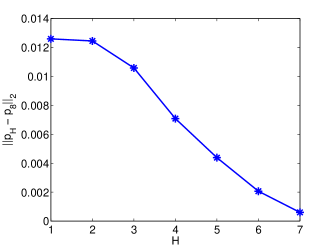
   (a)      (b)

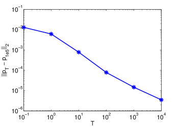
Fig. 5: (a) Convergence of the saFEM with $S=1$, $T=10^{5}$, $Q=0.1$, $B=10^{3}$, $\beta_{1}=0.01$ and $\beta_{2}=0.55$ over a range of mesh refinements $H$, for the system $\eqref{eq:lin}$. Errors are given by $(\ref{errorformula})$. (b) Convergence of the saFEM with $S=1$, $Q=10$, $B=10^{3}$, $\beta_{1}=0.01$, $\beta_{2}=0.4$, and $H=6$ over a range of SSA lengths $T$, for the system (20). Error is given by $(\ref{errorformula2})$.

Figure 5(a) shows the convergence of the method as the number of splits $H$ is increased from 1 to 7, where the error is calculated by comparison with an approximation using a mesh which has undergone up to 8 splits:

$$\mbox{Error}(H)=\left(\int_{\Omega}|p_{8}({\bf x})-p_{H}({\bf x})|^{2}{\mbox{d}{\mathbf{x}}}\right)^{1/2}.$$ (22)

When using a relatively coarse mesh, it is possible for the value of the approximation to be negative in regions. Since the function represents a probability density, which is strictly non-negative, this does not make sense. These negative areas can also complicate the normalisation of the function. We solve this problem by simply cutting off the negative values, i.e. we multiply the approximated function by the indicator function over the set where the function is non-negative, before normalising by (6).

7.3 Length of Stochastic Simulation

Next we show convergence of the method as $T$ is increased, with $S=1,$ $Q=10$, $B=10^{3}$, $\beta_{1}=0.01$, $\beta_{2}=0.4$ and $H=8$. As in the previous section, the SSA trajectory is given initial condition $(X_{1},X_{2},X_{3})=(120,100,100)$.

As the system is ergodic, we would expect that as the length of stochastic simulation increases and the number of samples increases, that our samples becomes increasingly representative of the invariant density in question. This gives us more information about where we should be refining our mesh, which in turn should give us a more accurate approximation.

Figure 5(b) shows the convergence of approximation as the length of stochastic simulation is increased. The error as plotted in Figure 5 (b) is the $L^{2}$ difference between the approximations with varying $T$ and the approximation calculated with $T=10^{5}$, namely:

$$\mbox{Error}(T)=\left(\int_{\Omega}|p_{10^{5}}({\bf x})-p_{T}({\bf x})|^{2}{\mbox{d}{\mathbf{x}}}\right)^{1/2}.$$ (23)

Note that in order to more easily compare the distributions, the domain selection for all of the data points was made using the longest stochastic simulation with $T=10^{5}$. This shows that as the simulation length is increased we see a convergence of the chosen mesh to one which well represents the region containing the invariant density.

7.4 Parameter $\beta_{1}$

In certain situations the stochastic simulations may be expensive and we may only be able to take a few samples from the stochastic trajectory. In this case we still have a large amount of uncertainty about the region which contains the vast majority of the invariant density. Therefore we can only hope to approximate this by increasing the size of the ellipsoid around each sampled point that we include in the region $\Gamma$ given by (15). Figure 6 shows the convergence of the method as $\beta_{1}$ is increased, with $S=1$, $T=10^{5}$, $Q=0.1$, $B=10^{3}$, $\beta_{2}=0.4$ and $H=6$.

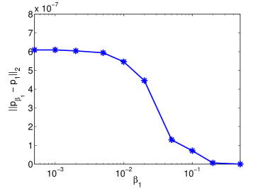
Fig. 6: Convergence of the saFEM with $\beta_{2}=0.4$, $Q=0.1$, $B=10^{3}$, $T=10^{5}$ and $S=6$ over a range of radii of uncertainty $\beta_{1}$, for the system (20). The error is defined by (24).

The error as plotted in Figure 6 is given by:

$$\mbox{Error}(\beta_{1})=\left(\int_{\Omega}|p_{1}({\bf x})-p_{\beta_{1}}({\bf x})|^{2}{\mbox{d}{\mathbf{x}}}\right)^{1/2}.$$ (24)

7.5 A numerical test of accuracy

In Section 5.3 a brief test for sufficient convergence was suggested, where two solutions were calculated, one with parameters

$$\{S,T,Q,B,\beta_{1},\beta_{2},H\},$$

and the second with parameters

$$\{S,2T,2Q,2B,2\beta_{1},\beta_{2},H+1\}.$$ (25)

If the two solutions are close up to some tolerance, then we can be fairly sure that the method has converged to a reasonable degree.

The solution for the system (20) calculated with the parameter set

$$\{S=1,\;T=10^{5},\;Q=0.05,\;B=500,\;\beta_{1}=10^{-3},\;\beta_{2}=0.45,\;H=7\},$$

when compared with the solution using the parameters

$$\{S=1,\;T=2\times 10^{5},\;Q=0.1,\;B=10^{3},\;\beta_{1}=2\times 10^{-3},\;H=8\},$$

gave $L^{2}$ error of $1.99\times 10^{-4}$, which is significantly less than the $L^{2}$ norm of the solution ($4.51\times 10^{-3}$). This gives a relative $L^{2}$ error of $4.41\times 10^{-2}$. For ease of comparison the domain $\Omega$ chosen using parameters (25) was used for both meshes.

7.6 Oregonator

Our final example is the Oregonator[22] which is a three species chemical system motivated by the Belousov-Zhabotinsky reaction. It exhibits oscillatory behaviour and is traditionally given by the following system of ODEs:

$$\frac{\mbox{d}x_{1}}{{\mbox{d}t}} = k_{1}x_{2}-k_{2}x_{1}x_{2}+k_{3}x_{1}-2k_{4}x_{1}^{2},$$

$$\frac{\mbox{d}x_{2}}{{\mbox{d}t}} = -k_{1}x_{2}-k_{2}x_{1}x_{2}+\frac{1}{2}k_{c}x_{3},$$ (26)

$$\frac{\mbox{d}x_{3}}{{\mbox{d}t}} = 2k_{3}x_{1}-k_{c}x_{3}.$$

We now construct a set of reactions whose behaviour is given by (26) in the thermodynamic limit:

$$X_{2}\;\displaystyle\mathop{\displaystyle\longrightarrow}^{k_{1}}\;X_{1}\qquad X_{1}+X_{2}\;\displaystyle\mathop{\displaystyle\longrightarrow}^{k_{2}}\;\emptyset \qquad X_{1}\;\displaystyle\mathop{\displaystyle\longrightarrow}^{k_{3}}\;2X_{1}+2X_{3}$$ (27)

$$2X_{1}\;\displaystyle\mathop{\displaystyle\longrightarrow}^{k_{4}}\;\emptyset \qquad X_{3}\;\displaystyle\mathop{-\!\!\!-\!\!\!-\!\!\!-\!\!\!-\!\!\!\!\displaystyle\longrightarrow}^{k_{5}=k_{c}/2}\;\emptyset \qquad X_{3}\;\displaystyle\mathop{-\!\!\!-\!\!\!-\!\!\!-\!\!\!-\!\!\!\!\displaystyle\longrightarrow}^{k_{6}=k_{c}/2}\;X_{2}.$$

Note that the reaction with parameter $k_{c}$ has been split into two reactions $R_{5}$ and $R_{6}$ in order to get the factor of half in the equation for the rate of change of $x_{2}$, with $k_{5}=k_{6}=k_{c}/2$. We consider this system with the following set of dimensionless parameters:

$$k_{1}=0.3,\quad k_{2}=4000,\quad k_{3}=5,\quad k_{4}=1200,\quad k_{c}=0.02.$$ (28)

In this parameter regime the stochastic description of these reactions exhibits oscillatory behaviour.

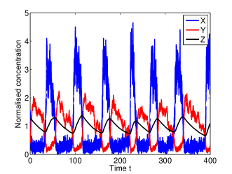
    (a)        (b)

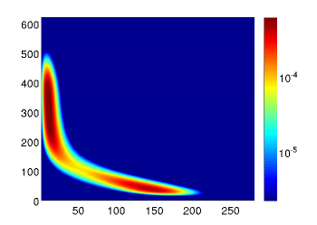
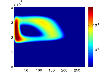
     (c)      (d)

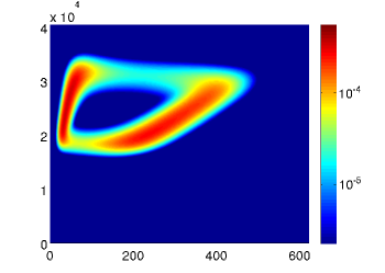
Fig. 7: (a) Trajectories of the Oregonator (27) with parameters given by (28), simulated using the Gillespie SSA. Plots show normalised trajectories, with actual molecule numbers divided by a time average ($47.7$, $211.5$ and $2.4\times 10^{4}$ resp.). (b)–(d) Approximation of the log of the marginal invariant distribution (conditioned on non-extinction of species $X_{1}$) of (27) with system parameters (28) in the (b) $x_{1}$-$x_{2}$ plane, (c) $x_{1}$-$x_{3}$ plane, (d) $x_{2}$-$x_{3}$ plane, by the saFEM with algorithmic parameters given by (29).

Figure 7(a) shows normalised trajectories of the Oregonator (27) with parameters given by (28), simulated using the Gillespie SSA. This figure demonstrates the oscillatory behaviour of the Oregonator in this parameter regime.

One thing of note should be mentioned at this point, regarding the ergodicity of this system. The zero state, at the origin, is an absorbing state for this system, and so trivially the invariant distribution for this system is a Dirac measure on this state. However, we are interested in the behaviour of this system conditioned on non-extinction of the species. Therefore we ensure that our domain of solution does not include this state, and thus the transient states involved in the oscillation behaviour now form the regions with non-zero invariant density.

In the figures that follow, these algorithmic parameters were used to approximate the steady state distribution (conditioned on non-extinction of species $X_{1}$):

$$S=1,\qquad T=10^{6},\qquad Q=10^{-2},\qquad B=10^{3},\qquad H=8$$ (29)

Since this system has a single limit cycle and is ergodic, step [1] of the algorithm (in Table 2) can be replaced by running the Gillespie SSA for a period of algorithm time until we are reasonably sure that the chain has entered probabilistic equilibrium, and using the endpoint of this simulation as the starting point for the SSA in step [2]. Since the system has a single stable orbit, we pick $S=1$. Since a priori we do not know a specific point on the most likely orbit, the initial condition $(x_{1},x_{2},x_{3})=(100,100,100)$ was chosen.

Since we wish to condition on non-extinction of all of the species, we must ensure that $X_{1}$ never drops below 1. We can do this by slightly altering the domain $\Omega$ of solution of the FPE. We do this by replacing the first line of (18) by $\Omega={\mathcal{A}}^{*}_{1}\times{\mathcal{A}}_{2}\times{\mathcal{A}}_{3},$ where

$${\mathcal{A}}^{*}_{1}=\left(\max\{1,x_{1}^{\rm min}-\beta_{2}\,x_{1}^{\rm range}\},x_{1}^{\rm max}+\beta_{2}\,x_{1}^{\rm range}\right).$$

The longer the simulation in the step [2] of the saFEM, the more sure we can be of the regions which have non-negligible probability density, and therefore the larger we can make $\beta_{2}$ and $\beta_{1}$. We choose $\beta_{1}=0.01$ and $\beta_{2}=0.1$.

Using these parameters, a mesh was created by the saFEM with $8.65\times 10^{5}$ vertices, out of a possible $1.70\times 10^{7}$ with up to 8 splits of each cuboid, with $1.17\times 10^{5}$ hanging nodes. Therefore there were a total of $7.48\times 10^{5}$ degrees of freedom, a mere $4.4\%$ of the degrees of freedom that would have been required to fill the domain with cuboids of the finest refinement level. The mesh contained $4.79\times 10^{6}$ individual tetrahedral elements.

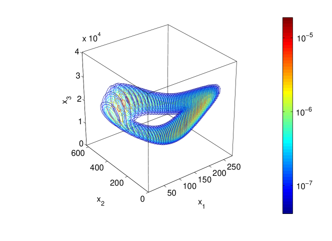
Fig. 8: Approximation of the invariant distribution (conditioned on non-extinction) of (27) with system parameters (28). Contours plots shown in several slices.

Figure 8 shows several slices of the approximated invariant probability density conditioned on non-extinction of species $X_{1}$, represented by contour plots. Since visualisation of a three-dimensional function on a two-dimensional page is problematic, we present also in Figure 7(b)–(d) the marginal densities of the approximation of the invariant density of the Oregonator system with parameters (28) in 3 different planes.

To verify that the method is accurately representing the invariant distribution, we can test the approximation as suggested in Section 5.3. The approximation was compared with one with the parameters given as follows:

$$S=1,\;T=5\times 10^{5},\;Q=5\times 10^{-3},\;B=5\times 10^{2},\;H=7,\;\beta_{1}=5\times 10^{-3}.$$

We omit $\beta_{2}$ here as the same domain as was chosen for the original parameter set was used for ease of comparison of the two densities. The $L^{2}$ difference between the two solutions was $2.89\times 10^{-11}$, with the original solution having an $L^{2}$ norm of $1.74\times 10^{-8}$, giving a relative $L^{2}$ error of $1.66\times 10^{-3}$, verifying that our solution is well converged.

8 Discussion

In this paper we have presented a method for solution of the steady-state Fokker-Planck equation for chemical systems. The method is based on the use of stochastic trajectories to estimate the region in which we must refine our finite element mesh the most. This method is only valid for systems which do not have large regions of the domain with non-negligible invariant density that can be accurately approximated by a linear function. Our assumption that regions which have high enough probability density require high levels of refinement would fail in this case, and the mesh produced would be inefficient.

The use of the Fokker-Planck equation as a means to model chemical reactions of the mesoscale has been present in the literature for some time[24, 36]. As computational resources have improved, the solving of such equations in more than one dimension has become tractable. It has been shown that using appropriate methods (such as finite volume methods), the solution of the Fokker-Planck equation is far more efficient than using an SSA for the computation of both time-dependent and steady state solutions, and with a high degree of accuracy[21, 36].

The Fokker-Planck equation does suffer badly from the curse of dimensionality, and many different methods exist which attempt to find approximations of the solution of these equations efficiently in more than one dimension. Some involve dimension reduction of the equations themselves, through simplifying assumptions, and through coupling with macroscopic reaction rate equations for some of the species[33]. Sparse grid methods have also been used in an attempt to find the invariant density of the chemical master equation[27]. Sparse grids attempt to overcome the curse of dimensionality by reducing greatly the number of degrees of freedom considered. This CME solution can also be coupled to Fokker-Planck equations for the more abundant species using a hybrid method[27]. Other methods have been used to approximate the solution of the chemical master equation, including adaptive wavelet compression[29] and finite state projection[34, 16].

There are several other ways that stochastic trajectories could be calculated in the saFEM, other than the standard SSA as detailed in Table 1. The $\tau$-leap method[26] approximates the trajectory by modelling several reactions in each iteration of the algorithm, up to a fixed time step. This can accelerate the simulation of the trajectory, but could incur some errors, including the possibility that the trajectory may become negative in one or more of the chemical species. Likewise, one could use numerical approximations of the chemical Langevin equation[25], a stochastic differential equation (SDE) with corresponding Fokker-Planck equation given by (3), to create trajectories. As with the $\tau$-leap method, the trajectories from this SDE can become negative, and so with both of these methods proper treatment of boundary conditions is key to accurately approximating the region of the positive quadrant that contains the majority of the probability density.

More information could also be extracted from the stochastic trajectories. A rudimentary approximation of the density could be made using the samples taken from the simulations, and used as a preconditioner for the eigensolver. As the eigensolver used is iterative, even a rough guess of the form of the solution could help to reduce computation times. It has been previously shown that combining stochastic simulations and solutions of differential equations can be used for preconditioning of computations[35].

Acknowledgements: The research leading to these results has received funding from the European Research Council under the European Community’s Seventh Framework Programme (FP7/2007-2013)/ ERC grant agreement No. 239870. This publication was based on work supported in part by Award No KUK-C1-013-04, made by King Abdullah University of Science and Technology (KAUST). The work of Simon Cotter was also partially supported by a Junior Research Fellowship of St Cross College, University of Oxford. Tomáš Vejchodský would like to acknowledge the support by the Grant Agency of the Academy of Sciences (project. IAA100760702) and the Academy of Sciences of the Czech Republic (institutional research plan no. AV0Z0190503). Radek Erban would also like to thank Somerville College, University of Oxford, for a Fulford Junior Research Fellowship; Brasenose College, University of Oxford, for a Nicholas Kurti Junior Fellowship; the Royal Society for a University Research Fellowship; and the Leverhulme Trust for a Philip Leverhulme Prize. This prize money was used to support a research visit of Tomáš Vejchodský in Oxford.

References

- [1] P. Amestoy, I. Duff, J. L’Excellent, and J. Koster. A fully asynchronous multifrontal solver using distributed dynamic scheduling. SIAM Journal on Matrix Analysis and Applications, 23(1):15–41, 2001.
- [2] P. Amestoy, A. Guermouche, J. L’Excellent, and S. Pralet. Hybrid scheduling for the parallel solution of linear systems. Parallel Computing, 32(2):136–156, 2006.
- [3] A. Arkin, J. Ross, and H. McAdams. Stochastic kinetic analysis of developmental pathway bifurcation in phage l-infected Escherichia coli cells. Genetics, 149:1633–1648, 1998.
- [4] I. Babuška and W. Rheinboldt. Error estimates for adaptive finite element computations. SIAM Journal on Numerical Analysis, 15(4):736–754, 1978.
- [5] S. Balay, J. Brown, K. Buschelman, W. Gropp, D. Kaushik, M. Knepley, L. McInnes, B. Smith, and H. Zhang. PETSc Web page, 2011. http://www.mcs.anl.gov/petsc.
- [6] S. Balay, W. Gropp, L. McInnes, and B. Smith. Efficient management of parallelism in object oriented numerical software libraries. In Modern Software Tools in Scientific Computing, pages 163–202, 1997.
- [7] L. Beilina, S. Korotov, and M. Křížek. Nonobtuse tetrahedral partitions that refine locally towards fichera-like corners. Applications of Mathematics, 50:569–581, 2005.
- [8] J. Bey. Tetrahedral grid refinement. Computing, 55:355–378, 1995.
- [9] Y. Cao, D. Gillespie, and L. Petzold. Multiscale stochastic simulation algorithm with stochastic partial equilibrium assumption for chemically reacting systems. Journal of Computational Physics, 206:395–411, 2005.
- [10] Y. Cao, D. Gillespie, and L. Petzold. The slow-scale stochastic simulation algorithm. Journal of Chemical Physics, 122(1):14116, 2005.
- [11] P. Ciarlet. The finite element method for elliptic problems. North-Holland Publishing Co., Amsterdam, 1978. Studies in Mathematics and its Applications, Vol. 4.
- [12] S. Cotter, T. Vejchodský, and R. Erban. Stochastic bifurcations of biochemical systems. in preparation, 2011.
- [13] S. Cotter, K. Zygalakis, I. Kevrekidis, and R. Erban. A constrained approach to multiscale stochastic simulation of chemically reacting systems. Journal of Chemical Physics, 135:094102, 2011.
- [14] M. Cowles and B. Carlin. Markov chain monte carlo convergence diagnostics: A comparative review. Journal of the American Statistical Association, 91(434):883–904, 1996.
- [15] E. Doedel, A. Champneys, T. Fairgrieve, Y. Kuznetsov, B. Sandstede, and X. Wang. AUTO 97: Continuation and bifurcation software for ordinary differential equations (with homcont), 1997.
- [16] B. Drawert, M. Lawson, L. Petzold, and M. Khammash. The diffusive finite state projection algorithm for efficient simulation of the stochastic reaction-diffusion master equation. Journal of Chemical Physics, 132:074101, 2010.
- [17] W. E, D. Liu, and E. Vanden-Eijnden. Nested stochastic simulation algorithm for chemical kinetic systems with disparate rates. Journal of Chemical Physics, 123:194107, 2005.
- [18] R. Erban, S. J. Chapman, I. Kevrekidis, and T. Vejchodsky. Analysis of a stochastic chemical system close to a sniper bifurcation of its mean-field model. SIAM Journal on Applied Mathematics, 70(3):984–1016, 2009.
- [19] R. Erban, S. J. Chapman, and P. Maini. A practical guide to stochastic simulations of reaction-diffusion processes. 35 pages, available as http://arxiv.org/abs/0704.1908, 2007.
- [20] R. Erban, I. Kevrekidis, D. Adalsteinsson, and T. Elston. Gene regulatory networks: A coarse-grained, equation-free approach to multiscale computation. Journal of Chemical Physics, 124:084106, 2006.
- [21] L. Ferm, P. Lötstedt, and P. Sjöberg. Conservative solution of the fokker-planck equation for stochastic chemical reactions. BIT Numerical Analysis, 46:61–83, 2006.
- [22] R. Field and R. Noyes. Oscillations in chemical systems. IV. limit cycle behavior in a model of a real chemical reaction. Journal of Chemical Physics, 60(5):1877–1884, 1974.
- [23] D. Gillespie. Exact stochastic simulation of coupled chemical reactions. Journal of Physical Chemistry, 81(25):2340–2361, 1977.
- [24] D. Gillespie. Approximating the master equation by Fokker-Planck equations for single-variable chemical systems. Journal of Chemical Physics, 72(10):5363–5370, 1980.
- [25] D. Gillespie. The chemical Langevin equation. Journal of Chemical Physics, 113(1):297–306, 2000.
- [26] D. Gillespie. Approximate accelerated stochastic simulation of chemically reacting systems. Journal of Chemical Physics, 115(4):1716–1733, 2001.
- [27] M. Hegland, A. Hellander, and P. Lötstedt. Sparse grids and hybrid methods for the chemical master equation. BIT Numerical Mathematics, 48(2):265–283, 2008.
- [28] V. Hernandez, J. Roman, and V. Vidal. SLEPc: A scalable and flexible toolkit for the solution of eigenvalue problems. ACM Transactions on Mathematical Software, 31(3):351–362, 2005.
- [29] T. Jahnke and T. Udrescu. Solving chemical master equations by adaptive wavelet compression. Journal of Computational Physics, 229(16):5724 – 5741, 2010.
- [30] S. Kar, W. Baumann, M. Paul, and J. Tyson. Exploring the roles of noise in the eukaryotic cell cycle. Proceedings of the National Academy of Sciences USA, 106:6471–6476, 2009.
- [31] S. Korotov and M. Křížek. Acute type refinements of tetrahedral partitions of polyhedral domains. SIAM Journal on Numerical Analysis, 39(2):724–733, 2002.
- [32] V. Kublanovskaya. On some algorithms for the solution of the complete eigenvalue problem. U.S.S.R. Computational Mathematics and Mathematical Physics, 1(3):555–570, 1961.
- [33] P. Lötstedt and L. Ferm. Dimensional reduction of the fokker-planck equation for stochastic chemical reactions. Multiscale Modelling and Simulation, 5:593–614, 2006.
- [34] B. Munsky and M. Khammash. The finite state projection algorithm for the solution of the chemical master equation. The Journal of Chemical Physics, 124(4):044104, 2006.
- [35] L. Qiao, R. Erban, C. Kelley, and I. Kevrekidis. Spatially distributed stochastic systems: Equation-free and equation-assisted preconditioned computation. Journal of Chemical Physics, 125:204108, 2006.
- [36] P. Sjöberg, P. Lötstedt, and J. Elf. Fokker-planck approximation of the master equation in molecular biology. Computing and Visualization in Science, 12:37–50, 2009.
- [37] P. Šolín, J. Červený, and I. Doležel. Arbitrary-level hanging nodes and automatic adaptivity in the -FEM. Mathematics and Computers in Simulation, 77(1):117–132, 2008.
- [38] R. Verfürth. A review of a posteriori error estimation and adaptive mesh-refinement techniques. Chichester: John Wiley & Sons. Stuttgart: B. G. Teubner., 1996.
- [39] J. Villar, H. Kueh, N. Barkai, and S. Leibler. Mechanisms of noise-resistance in genetic oscillators. Proceedings of the National Academy of Sciences USA, 99(9):5988–5992, 2002.
- [40] C. Zenger. Sparse grids. In W. Hackbusch, editor, Parallel algorithms for partial differential equations, volume 31 of Notes on Numerical Fluid Mechanics, pages 241–251. Vieweg-Verlag, 1991.