Towards Uncertainty Quantification and Inference in the stochastic SIR Epidemic Model

Abstract

In this paper we introduce a novel method to conduct inference with models defined through a continuous-time Markov process, and we apply these results to a classical stochastic SIR model as a case study. Using the inverse-size expansion of van Kampen we obtain approximations for first and second moments for the state variables. These approximate moments are in turn matched to the moments of an inputed generic discrete distribution aimed at generating an approximate likelihood that is valid both for low count or high count data. We conduct a full Bayesian inference to estimate epidemic parameters using informative priors. Excellent estimations and predictions are obtained both in a synthetic data scenario and in two Dengue fever case studies.

1 Introduction

Stochasticity and nonlinearity have a major role in shaping the dynamics of epidemics of infectious diseases. It is known that the effects of demographic stochasticity weight more in determining the dynamics of epidemics when the number of individuals in the population is low. Consequently, the development of mathematical epidemic models that take into account uncertainty and are amenable to describing small populations is an active field of research, see [1, 2, 3, 4, 5, 6]. Among these modeling efforts, models based on Markov processes have received a lot of attention. It has been argued that continuous-time discrete-space (CTDS) Markov processes whose forward-Kolmogorov equation is known as the chemical master equation (CME) represent the stochastic counterpart to systems of ordinary differential equations [7], and are often referred to as birth-and-death processes. The research presented in this paper is based on this modeling paradigm. We consider the stochastic SIR epidemic model as a case study. The SIR model and its variants are ubiquitous in the study of dynamics of epidemics in populations of plants and animals [8, 9]. Seasonality, migration, vaccination, demographic and environmental stochasticity are among the epidemics features that give rise to variants of the SIR model. There is a wealth of qualitative results that have been obtained from the analysis of these models, e.g. thresholds for the onset of epidemics, amplification of environmental and demographic noise, mechanisms for local extinction and invasion of epidemics. Feedback from the bifurcation analysis of deterministic SIR models  [10, 11, 12, 13] and the analysis of the interplay of stochasticity and nonlinearity [14, 15] has provided substantial insight regarding epidemic dynamics. A related topic is the quantitative study of the predictive capacity of epidemic models. Recently, parameter estimation of epidemic models, from a time series analysis perspective, and with varying degrees of formality have been attempted [16, 17, 18, 19, 20].

Recently, various Bayesian and likelihood based approaches to parameter inference in CME type models have been attempted. Some authors have tried to work with a deterministic, continuous or steady state alternative model to infer the parameters in the CME [21, 22], but with modest success; specially in the important scenario of low number of counts for the species, when the stochastic evolution of the system is in fact the main object of interest [23]. In particular, previous research efforts to conduct Bayesian inference with the CME include [24, 22], where the CME is approximated by a diffusion process and [25] where the van Kampen expansion is used to derive a diffusion approximation; other similar papers include [26, 27]. However, this approach applies when individual counts are large and, in the limit, fluctuations are small and in turn approximated with a Gaussian diffusion [26, p. 246] which, certainly, will be of limited use if the low counts for some or all species are an issue, as it is the case with epidemic studies.

In the chemical master equation scenario simulating data is possible (see Section 2) and the likelihood free Approximate Bayesian Computational (ABC) inference ideas may be used [28]. The ABC simulates data for fixed parameters and rejects trajectories that are not “close” (according to an ad hoc metric among an ad hoc statistic) to available data. However, as of yet the ABC lacks of a firm theoretical support and many crucial details remain unknown, namely, what regularity conditions are required (if any) for the ABC to work, how to choose the tolerance and metric and the consequences of not using a sufficient statistic [28]. Moreover, when the number of reactions per unit of time increases the simulation algorithm may become very inefficient. [29] represents an attempt to use the ABC in this context, for model inference and model selection; however a very recent result [30] will severely question the validity of the latter. Other Bayesian inference approaches for the CME are [31, 32] and will be discussed in further detail in Section 3.

In this paper we describe a method to conduct parameter estimation in the CME from partial observation of the state variables. We have used the van Kampen expansion to obtain approximate equations of the dynamics of the first two moments of the state variables of the CME to impute a counting model matching these moments to create a likelihood for Bayesian inference. We remark that our results hold for low populations. For the sake of clarity, our examples use the simplest epidemic model, e.g. the SIR model without vital dynamics. It is shown that inference is possible with the approximate likelihood using synthetic data generated with the Gillespie algorithm and the stochastic SIR model. We offer results with data from Dengue Fever onset from two cities central Mexico, Acapulco in 2005 and Cuernavaca in 2008. Our contention is that the results presented in this paper hold for models formulated as a CME under the hypothesis of spatial homogeneity and thermodynamic equilibrium, where only mono-molecular and bimolecular reactions occur.

The paper is organized as follows. In the next section we explain the SIR model and the moment approximations that we have used, in Section 3 we explain the details of the Bayesian inference and in Sections 4 and 5 we present examples with synthetic and real data, respectively. In Section 6 a discussion of the paper is presented.

2 The Stochastic SIR model and moment approximations

Gardiner [33] claims that it is appropriate to describe the dynamics of intrinsically discrete systems such as epidemics in terms of jumps. Also, establishes that the chemical master equation (CME) offers a complete description of such systems since the CME embodies macroscopic deterministic laws of motion about which of the stochastic nature of the system generates a random part. However, the chemical master equation accounts only for local (demographic) sources of stochasticity. Presumably, a complete model of an ecological system such as epidemics should also account for global (environmental) sources of stochasticity such as weather. Nevertheless, a general framework to derive stochastic models that takes into account both sources of stochasticity is not available. Although it is possible to couple the chemical master equations with models of extrinsic noise [1, 6], in this paper we restrict ourselves to the CME of the classical SIR epidemic model to conduct Bayesian inference.

We present briefly the CME as in [32]. For $u$ ‘species’ $\mathbf{X}=(X_{1},\ldots,X_{u})$ and $v$ ‘reactions’ it is assumed that for a small enough time interval $\Delta t$ only one of the following $v$ reactions takes place

$$R_{k}:p_{k1}X_{1}+\ldots+p_{ku}X_{u}\stackrel{{\scriptstyle h_{k}}}{{\longrightarrow}}q_{k1}X_{1}+\ldots+q_{ku}X_{u}$$

where $k=1,2,\ldots,v$ and $p_{kj}$ is the ‘stoichiometry’ of reactant $j$ in reaction $k$ and $q_{kj}$ is the ‘stoichiometry’ of product $j$ in reaction $k$, see [32] for more details. This means that if reaction $k$ takes place $X_{j}$ changes by $q_{kj}-p_{kj}$. Each reaction $R_{k}$ has an associated reaction rate $h_{k}(\mathbf{X},\theta_{k})$ (we assume here that $\theta_{k}$ is a real positive parameter). Once a reaction has occurred (or at $t=0$) the time to the next reaction has an exponential distribution with rate $h_{0}(\mathbf{X},\theta_{k})=\sum_{k=1}^{v}h_{k}(\mathbf{X},\theta_{k})$, and the $k$th reaction occurs with probability $h_{k}(\mathbf{X},\theta_{k})/h_{0}(\mathbf{X},\theta_{k})$. This constitutes a pure Markov jump process (continuous time) and since only the exponential and a discrete distribution is involved it is straightforward to simulate from; this is the so called Gillespie simulation method [34]. The probability law governing the behavior of this Markov process is the CME. This model has been applied in a diversity of fields, e.g. biochemical reactions [35], viral infections [36] and ecology [37]. Although in the following we concentrate on a much simpler setting (the SIR model) we keep this general model in perspective. In fact, our inference and prediction procedure may be considered in this general setting as far as the rates $h_{k}(\mathbf{X},\theta_{k})$ are polynomial, i.e. Kurtz theorem for the Fokker-Plank approximation holds, see Gardiner [33].

2.1 The SIR model

As mentioned in Section 1, here we will work on a simple epidemic of the SIR type (susceptible, infectious, recovered). The stochastic approach to modeling epidemics has a long history and dates back to the pioneering work of Kermack and McKendrick [38, 39, 40]. The main hypothesis of the model is that contact rates occur according to a mass-action law and there is no demographic dynamics, implying that the time scale of the model is the length of a single epidemic event. The classical approach has been particularly valuable when small population sizes do not support the assumptions of the deterministic ODE models. The reader is referred to Daley and Gani [41] for a classical and standard derivation of the basic SIR epidemic model.

Let the random variables $X_{1}$, $X_{2}$ and $X_{3}$ denote respectively the ( ‘ ‘species”) number of susceptible, infected and recovered individuals in a closed population. The stochastic model is defined by two possible “reactions”: infection and removal, which occur with “propensities” (rates) $h_{1}$ and $h_{2}$ respectively:

$$R_{1}:X_{1}+X_{2} \stackrel{{\scriptstyle h_{1}}}{{\longrightarrow}}2X_{2}\qquad\text{infection}$$

$$R_{2}:X_{2} \stackrel{{\scriptstyle h_{2}}}{{\longrightarrow}}X_{3}\qquad\text{removal}.$$

Here we have $v=3$ species and $u=2$ reactions. The reaction rates are given by $h_{1}(X_{2},b_{0})=b_{0}X_{2}/\Omega$ and $h_{2}=b_{1}$, for some positive parameters $b_{0},b_{1}$ and $\Omega$ to be explained below.

If we denote by $\mathbf{x}=(x_{1},x_{2},x_{3})$ a realization of the random variables $\mathbf{X}=(X_{1},X_{2},X_{3})$, and let $P_{(x_{1},x_{2},x_{3})}(t)$ be the probability that the system is in state $\mathbf{x}=(x_{1},x_{2},x_{3})$ at time $t$, then the chemical master equation for this system is given by

$$\begin{split}\frac{dP_{(x_{1},x_{2},x_{3})}(t)}{dt}&=b_{0}\frac{(x_{2}-1)}{\Omega}(x_{1}+1)P_{(x_{1}+1,x_{2}-1,x_{3})}(t)\\ &+b_{1}(x_{2}+1)P_{(x_{1}+1,x_{2}-1,x_{3}-1)}(t)\\ &-(b_{0}\frac{x_{2}}{\Omega}x_{1}+b_{1}x_{2})P_{(x_{1},x_{2},x_{3})}(t).\end{split}$$ (1)

Let

$$x_{1} =\Omega y_{1}+\Omega^{1/2}z_{1}$$

$$x_{2} =\Omega y_{2}+\Omega^{1/2}z_{2}$$

$$x_{3} =\Omega y_{3}+\Omega^{1/2}z_{3},$$

where $y_{i}$ y $z_{i}$, $i=1,2,3$ are respectively realizations of the means $Y_{i}$ and the fluctuations $Z_{i}$ of the state variables $X_{i}$. Applying the van Kampen’s inverse size expansion [33] to equation (1) leads to (deterministic) differential equations for the dynamics of the means

$$\dot{y}_{1} =-b_{0}\frac{y_{2}}{\Omega}y_{1}$$ (2)

$$\dot{y}_{2} =b_{0}\frac{y_{2}}{\Omega}y_{1}-b_{1}y_{2}$$ (3)

$$\dot{y}_{3} =b_{1}y_{2}.$$ (4)

Equations (2)-(4) represent the macroscopic limit of the CME, and coincide with the classical deterministic SIR model. From the van Kampen’s expansion we obtain also a linear Fokker-Plank partial differential equation governing the dynamics of the fluctuations of the state variables

$$\dot{\Psi}=-\sum_{i,j}A_{ij}\frac{\partial}{\partial z_{i}}(z_{j}\Psi)+\frac{1}{2}\sum_{i,j}B_{ij}\frac{\partial^{2}\Psi}{\partial z_{i}\partial z_{j}},$$ (5)

where

$$A=\begin{pmatrix}-b_{0}y_{2}&-b_{0}y_{1}&0\\ -b_{0}y_{2}&-b_{0}y_{1}-b_{1}&0\\ 0&b_{1}&0\end{pmatrix},$$

$$B=\begin{pmatrix}b_{0}y_{1}y_{2}&-b_{0}y_{1}y_{2}&0\\ -b_{0}y_{1}y_{2}&b_{0}y_{1}y_{2}+b_{1}y_{2}&-b_{1}y_{2}\\ 0&-b_{1}y_{2}&b_{1}y_{2}\end{pmatrix},$$

and $\Psi=\Psi(z_{1},z_{2},z_{3},t)$ is the probability that the fluctuations are in state $(z_{1},z_{2},z_{3})$ at time $t$, see [42, 5]. From equation (5) it can be readily established [5] that the first and second moments of the fluctuations obey the following differential equations

$$\frac{d\mathbb{E}[z_{k}]}{dt} =\sum_{k}^{3}A_{ik}\mathbb{E}[z_{k}]$$ (6)

$$\frac{d\mathbb{E}[z_{i}z_{j}]}{dt} =\sum_{k}^{3}A_{ik}\mathbb{E}[z_{k}z_{j}]+\sum_{k}^{3}A_{jk}\mathbb{E}[z_{i}z_{k}]+B_{ij},$$ (7)

for $i,j,k=1,2,3$. In the following sections, we shall use equations (6)-(7) to impute a counting model aimed at conducting Bayesian inference with the CME.

2.2 Synthetic data

In order to generate synthetic trajectories of the stochastic SIR model in exact accordance with the CME a simulation method was outlined in Section 2, namely the Gillespie simulation algorithm [34]. For a moderate number of reactions, the Gillespie algorithm is feasible. A sub sampling of the resulting trajectories will generate data exactly distributed as the CME model. We will use this procedure to simulate synthetic data in Section 4. However, the moment approximations in (2)-(7) are used to impute a model for the data and this is used to perform our inferences. This in fact avoids the testing strategy known as “inverse crime”, see [43], where the same theoretical ingredients are used to synthesize and to invert data (infer parameters) in an inverse problem. We explain this inference procedure in the next Section.

3 Bayesian inference and MCMC

Recently, various Bayesian and likelihood based approaches to parameter inference in CME type models have been attempted. Some have tried to work with a deterministic, continuous or steady state alternative model to infer the parameters in the CME [21, 22], but with modest success; specially in the most important scenarios with low number of counts for the species, when the stochastic evolution of the system is in fact the main object of interest [23, 32]. Note that, in the artificial extreme case when observations are available for all reactions in all species inference is straightforward since the problem becomes one of estimating the rates in exponential sampling. If in addition it is assumed that the reaction rates have the form $h_{k}(\mathbf{X},\theta_{k})=\theta_{k}g_{k}(\theta_{k})$ even a simple (Gamma) Bayesian conjugate inference can be conducted [32].

Indeed, data is never complete in real CME applications and the inference problem could be regarded as one of missing data [44]. [32] takes the latter perspective to develop a full Bayesian approach. A consistent handling of missing data is available in the Bayesian paradigm were a complete data set is simulated from the predictive distribution of missing data given the actual observations and, in turn, the unknown parameters are simulated form the complete data posterior (the analytic version of this is totally out of the question in this context). This creates a two stage sampling procedure that would generate samples from the correct posterior distribution. The problem in this context is simulating complete data sets given observations at fixed time points of typically few (or just one) of the species. This would mean generalizing the Gillespie simulation algorithm to force all trajectories to pass through the count observations available for each species. As opposed to the simplicity of the original Gillespie algorithm, this additional complication renders the missing data simulation very complex and apparently no direct simulation method is available. [32] attempt two algorithms to approach this missing data simulation creating a rather complex MCMC. Even in the case of a very simple two species three reaction CME they obtain partial success when considering some prior settings and it is indeed not clear how this MCMC will generalize to other different or more complex CME’s [32].

Since simulating data is possible, the likelihood free ABC inference ideas may be used [28]. However, as mentioned above, the ABC lacks of a firm theoretical support and many crucial details remain unknown, namely, what regularity conditions are required (if any) for the ABC to work, how to choose the tolerance and metric, and the consequences of not using a sufficient statistic [28]. Moreover, when the number of reactions per unit of time increases the Gillespie algorithm may become very inefficient.

Here we take a novel approach to performing Bayesian inference for parameters in the CME, different in many respects to the previous approaches outlined above. We use the moment approximations in (6)-(7) to impute a counting data model for available observations matching those moments, to create an imputed likelihood to perform our inference. That is, instead of considering the full Bayesian missing problem approach, we build an approximate data model from which inference is much simplified. Nonetheless, our examples show that inference and trajectory prediction in the true CME is possible when using our approximate likelihood. Although the Kramer-Moyal moment approximation would provide similar results as (6)-(7) [see 33, chapter 7], the van Kampen approximation outlined in Section 2 has a firmer theoretical background, and will apply for rate functions common in ‘chemical’ reactions (as those considered here). Furthermore, the only critical assumption is that the system (the total number of species counts) is large [33], which is precisely the case in epidemic models. That is, individual counts can indeed be low at specific time points, but the system size $\Omega$ remains large (say $\geq 100$), which in closed population epidemic models (like the SIR model) remains constant and equal to the population size. There is also the moment closure approach [34, 45] for which a Bayesian inference has also been attempted [31], but assumes a specific moment structure and is neither suited to handle low species counts.

3.1 Approximate Likelihood

We assume the difficult case in which only one species is observed. In most applications of the SIR model explained in Section 2 only the number of Infectious individuals at some fixed time points are observed (in fact, in some real situation only an approximation for the latter is available, see Section 3.3). That is, let $t_{1},t_{2},\ldots,t_{n}$ be some observation time points and $\mathbf{D}=(x_{2}(t_{1}),x_{2}(t_{2}),\ldots,x_{2}(t_{n}))$ the data available.

We define a Generic Discrete Distribution $Gd(m,v)$, that is a combination of the commonly used counting data models, namely, the Binomial, the Poisson and the Negative-Binomial, and is explained in detail in [46]. For any mean and variance $\mu,v>0$ we make a combination of these three distributions in the following way

$$Gd(x|\mu,v)=\begin{cases}C_{x}^{m}~{}p^{x}(1-p)^{m-x};~{}&\text{if}~{}~{}\mu>v\\ e^{-v}\frac{v^{x}}{x!};~{}&\text{if}~{}~{}\mu=v\\ C_{x-1}^{x+m-1}~{}p^{x}(1-p)^{m};~{}&\text{if}~{}~{}\mu<v\\ \end{cases}$$ (8)

where $x\in\mathbb{N}$, $p=1-\min\left\{\frac{m}{v},\frac{v}{m}\right\}$, $m=\frac{\mu^{2}}{|\mu-v|}$ and $C_{x}^{m}$ are the combinations of $m$ items taken in subsets of size $x$. That is, we use a Binomial if $\mu>v$, a Poisson if $\mu=v$ and a Negative-Binomial if $\mu<v$. Neither of these distributions can handle any mean and variance; by combining these distributions we obtain the Generic Discrete class $Gd(\mu,v)$ defined for arbitrary mean $\mu$ and variance $v$, $\mu,v>0$, and these two moments completely define the distribution. Indeed, it is straightforward to see that if $X\sim Gd(\mu,v)$, $E(X)=\mu$ and $V(X)=v$. More importantly, for a fixed mean $\mu$, given both the properties of the Binomial and the Negative-Binomial, we see that $\lim_{v\rightarrow\mu}Gd(x|\mu,v)=e^{-v}\frac{v^{x}}{x!}.$ Therefore we have a continuous evolution of this parametric class, being the Poisson the “continuous bridge” between the Binomial ($\mu>v$) and Negative Binomial ($\mu<v$). (Note that if $\mu>v$ and $v\rightarrow\mu$, the support will increase to cover all $\mathbb{N}$ since $m\rightarrow\infty$.) Moreover, if $X\sim Gd(\mu,v)$, $\frac{X-\mu}{\sqrt{v}}$ will tend to a standard Normal distribution if $\mu\rightarrow\infty$ and $p\rightarrow p_{0}\in(0,1)$. That is, for large $\mu$, large counts, (and for example $\mu-3\sqrt{v}>0$) $Gd(\mu,v)$ can be approximated with a $N(\mu,v)$.

From (6)-(7) we assume that $\mathbb{E}[X_{2}(t)|b_{0},b_{1},\Omega]=m_{t}$ and $\mathbb{V}[X_{2}(t)|b_{0},b_{1},\Omega]=v_{t}$ are readily available be numerically solving the referenced system of differential equations. We assume that

$$X_{2}(t_{i})\mid b_{0},b_{1},\Omega\sim Gd(m_{t_{i}},v_{t_{i}})$$ (9)

(If observations for more species were available, a multivariate generic discrete distribution is also explained in capistran2011generic [46] which can be used to define their joint distribution using the cross moments in (7)).

Certainly, observations are taken at time points and since we are dealing with a Markov process these are not independent in general. The time lagged cross moments $\mathbb{E}[X_{2}(t)X_{2}(t+h)]$ would be very useful in defining the discrete joint distribution for observations, but these moments cannot be calculated in any way similar to the moments in (6)-(7). Note, however, that the model in (9) is only an approximation, imputed to match the available moments and, as approximations go, we may as well take their joint distribution as

$$l(\mathbf{D};b_{0},b_{1},\Omega)=\prod_{i=1}^{n}Gd(x_{2}(t_{i})|m_{t_{i}},v_{t_{i}}).$$

Consequently our approximate likelihood is defined as the product of individual distributions, as if the observations were independent. We present in the next section the corresponding prior and posterior distributions. The use and validity of this approximate likelihood will only be pondered when we show to recover the true parameter values in a synthetic data scenario, Section 4, and prove its predictive capability in real data examples, in Section 5.

3.2 Posterior distribution, MCMC and prediction

Since $b_{0},b_{1}$ and $\Omega$ are positive parameters, we use a Gamma distribution as a default and flexible family of priors for these parameters, namely

$$b_{0}\sim Ga(\alpha_{0},\beta_{0}),~{}~{}b_{1}\sim Ga(\alpha_{1},\beta_{1})~{}~{}\text{and}~{}~{}\Omega\sim Ga(\alpha_{2},\beta_{2}),$$ (10)

for known hyper-parameters $\alpha_{i},\beta_{i}$. The log-posterior distribution is therefore

$$\begin{split}\log f(b_{0},b_{1},\Omega|\mathbf{D})&=C+\sum_{i=1}^{n}\log Gd(x_{2}(t_{i})|m_{t_{i}},v_{t_{i}})\\ &+\sum_{j=0}^{1}(\alpha_{j}-1)\log(b_{i})-\beta_{i}b_{i}\\ &+(\alpha_{2}-1)\log(\Omega)-\beta_{2}\Omega,\end{split}$$

for some unknown normalizing constant $C$, $b_{0},b_{1},\Omega>0$. In some situations the total population size $\Omega$ is known and the posterior distribution will depend on the parameters $b_{0}$ and $b_{1}$ only by fixing the (log) posterior to $\Omega=N$, for some fixed population size $N$.

The likelihood depends on the parameters $b_{0},b_{1},\Omega$ through the moments $m_{t_{i}},v_{t_{i}}$. For any fixed parameter settings, evaluating the likelihood therefore represents numerically solving the differential equations in (6)-(7). Indeed, no analytical alternative is available and therefore we resort to MCMC simulation techniques [47].

Since no analytical version is available for the posterior distribution, the full conditional distributions cannot be calculated and usual approaches like the Gibbs sampler are impossible to implement. Conventional Metropolis-Hastings MCMC, like a random walk MH [47], are difficult to design and use. Even a fine tuned MCMC for a particular example may fail radically with the simplest modification. We use instead a self adjusted MCMC that automatically tunes itself and has been proved to be of great use in a variety of situations. Namely, we use the t-walk [48] MCMC sampler (for continuous parameters) which only requires the log posterior distribution and two initial points for the parameters of interest. In many examples, those shown below and many others, the t-walk works quite well in this two or three parameter MCMC simulation problem.

It is very interesting and useful to predict future observations of species; specially in the case of the epidemic example presented in Section 5, where the ability to predict the evolution of the epidemic in the near future may well be a crucial piece of information for public health decision makers. In Bayesian statistics the marginal posterior distribution of observables is calculated to make predictions (i.e.. the posterior predictive distribution). In this approximate likelihood setting and once the (t-walk) MCMC sample for our parameters is available, $b_{0}^{(h)},b_{1}^{(h)},\Omega^{(h)},h=1,2,\ldots,H$, simulating posterior predictive samples for $x_{2}(t_{n+1})$ is straightforward by simulating from $Gd(m_{t_{n+1}}^{(h)},v_{t_{n+1}}^{(h)})$. That is, for each of the specific parameter settings $b_{0}^{(h)},b_{1}^{(h)},\Omega^{(h)}$ the moment approximations are also calculated at the future time $t_{n+1}$ and a (predictive) simulated value $x_{2}^{(h)}(t_{n+1})$ is generated by simulating from the Generic Discrete distribution, $Gd(m_{t_{n+1}}^{(h)},v_{t_{n+1}}^{(h)})$, explained in Section 3.1

3.3 Handling surveillance epidemic data

Our aim is to use epidemics surveillance data to make our inferences. According to Diekmann and Heesterbeek [49] prevalence is the number of cases notified up to a given time t, and time is measured in some arbitrary scale. On the other hand, the incidence is the expected value of the number of new cases per unit time. In order to circumvent the difficulty of using surveillance data to estimate the model parameters we have assumed that data is proportional to incidence.

We assume that the actual number of infectious individuals at reporting times satisfies $x_{2}(t_{i})=kr(t_{i})$ where $k$ is an unknown constant and $r(t_{i})$ are the number of reported cases at time $t_{i}$. That is, the number of infectious people is proportional to the number of reported cases. Moreover, the initial number of susceptibles $x_{1}(0)=\Omega-x_{2}(0)$ is also unknown. Since $k$ is unknown, it is confounded with $\Omega$. We simply take $\Omega$ as an unknown (now instrumental) parameter in our model and take $x_{2}(t_{i})=r(t_{i})$. This pragmatic approach avoids further complicating the model and inference and in our synthetic data examples permits reconstructing $b_{0}$ and $b_{1}$ even when $\Omega$ is also unknown.

In the examples that we study below cases are reported monthly or weekly and are confirmed through an official detection algorithm approved by the Federal Health Secretariat of Mexico. In this respect the Cuernavaca data is probably the one better monitored since information on each case is more complete (age, sex, address, reference numbers, dates of admission to healthcare, etc are provided). Nonetheless, both examples are only meant to test our methods and therefore show probably two typical cases of the extremes of data quality and availability. In a forthcoming paper we will be more concerned with the actual population dynamics of the disease where a more detailed data selection and treatment is necessary.

4 Example: Synthetic Data

In this section we offer synthetic examples aiming at showing the accuracy and predictive features of the inference methods developed in the previous sections. For the sake of conciseness, we restrict ourselves to two contrasting cases. First, we set $\Omega=200$ and use many data points to solve the inference problem, see Figure 1. In the second example $\Omega$ is regarded as unknown (also a parameter) and many data points are trimmed out of the analysis. Furthermore, some data points are predicted, see Figure 2. In both examples synthetic data was created with the Gillespie algorithm mentioned above and fixed parameter values to $b_{0}=40$ and $b_{1}=7$.

By using the formalism of the CME we are allowing for stochastic fluctuations in the state variables that, in the case of the SIR model, refer to demographic stochasticity due to individual differences in contact rates ($b_{0}$) and time of infectiousness ($b_{1}$). In Figure 1(d) we present the posterior distribution for $R_{0}$ which, therefore, approximates the distribution of $R_{0}$ among individuals in the population. The Maximum a posteriori (MAP, the posterior mode) estimator for $R_{0}$ is 6.0, with $(4.8,7.0)$ as Highest Posterior Density 95% probability interval [HPD, an interval accumulating 0.95 probability with minimum length, the Bayesian equivalent of ‘credible’ intervals, see 50]. Model predictions follow the true epidemic behavior with reasonable accuracy (see Figure 1(a)). In this experiment the full data set was used.

To test for robustness we performed a new run but trimming away the last 14 weeks of the epidemic and considered the total population size $\Omega$, as unknown. Essentially we are only using the information necessary for the estimation of $R_{0}$. Model predictions are presented in Figure 2(a). The capacity of the model to predict the epidemic tail is remarkable although, as expected, the uncertainty on the estimation of $R_{0}$ increases relative to the previous case, moreover, its posterior distribution is quite skewed, see Figure 2(d). However, although in this case the MAP estimator for $R_{0}$ is 2.9, its posterior mean is 6.3, quite similar to the estimator of $R_{0}$ in the complete data, known $\Omega$, previous example. The 95% HPD probability interval is $(2.9,16.2)$. Note that for this skew distribution a single estimator is a very bias representation of the posterior distribution. Unlike all other posterior densities presented here the MAP and posterior mean differ in this case. The posterior distribution itself should always be used for a better interpretation in this Bayesian analysis [a point that went unnoticed in 51].

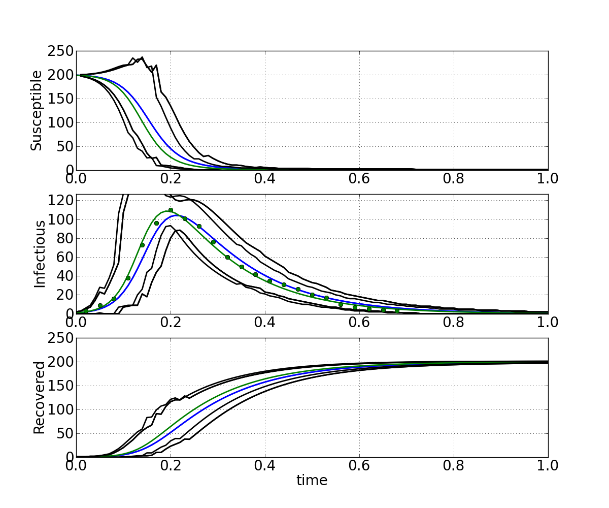
(a)

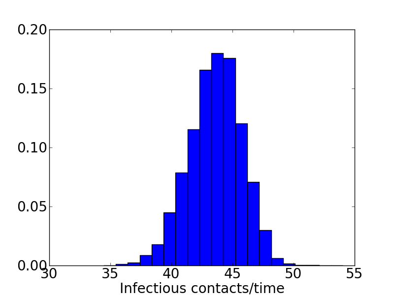
(b)

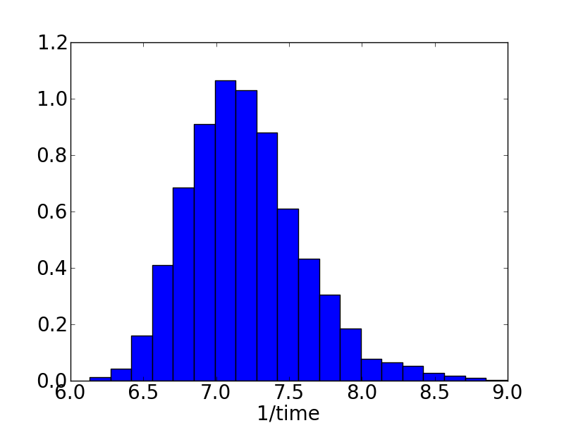
(c)

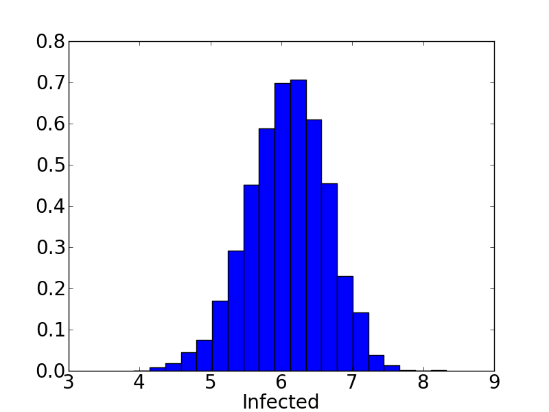
(d)

Figure 1: Synthetic data with $b_{0}=40,b_{1}=7$ and $N=200$. (a) True model (blue) and MAP estimated model (green) and 5% and 95% quantile bands for the imputed $Gd$ distribution at any time. Posterior distributions for $b_{0}$ (b), $b_{1}$ (c) and $R_{0}$ (d).

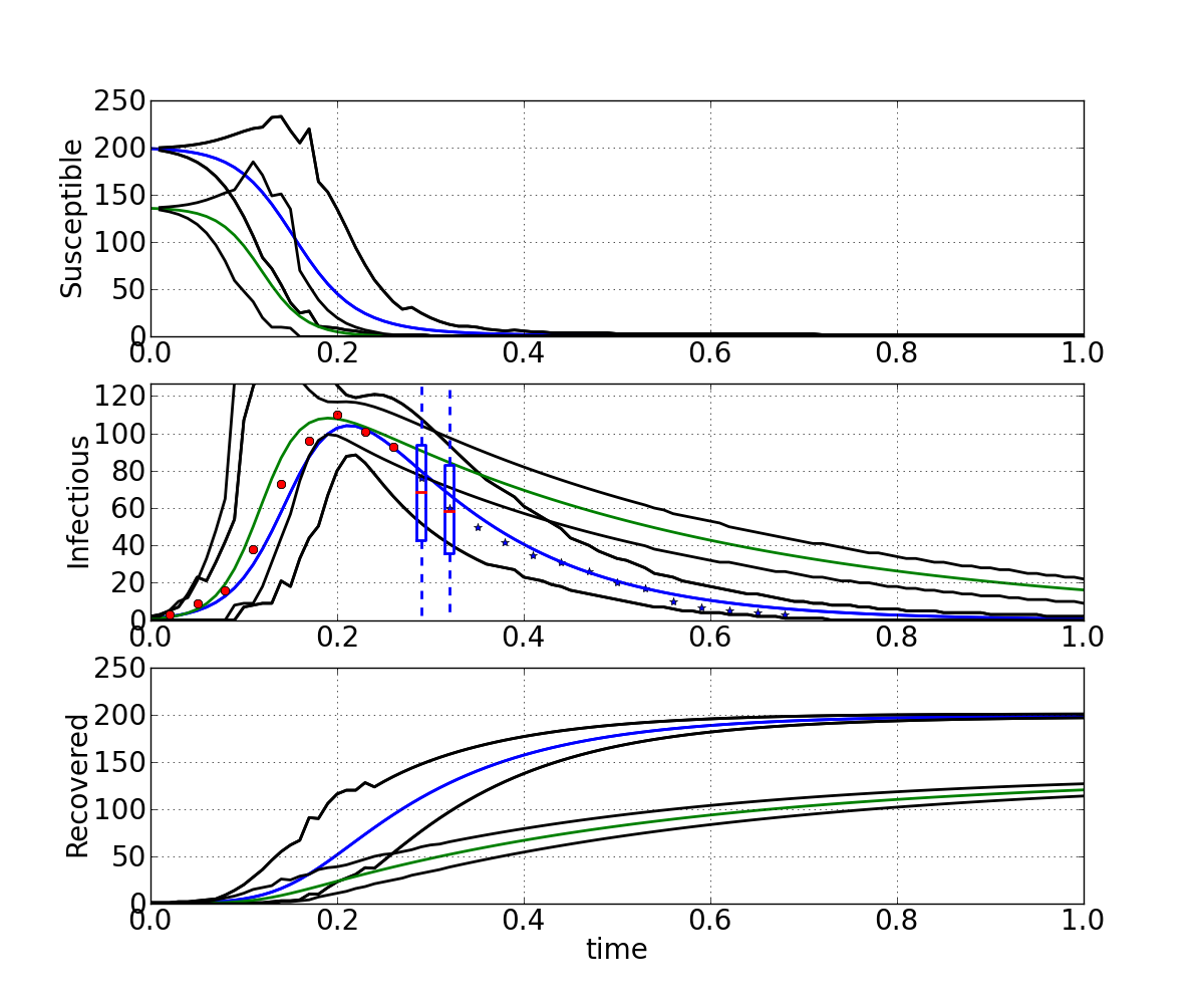
(a)

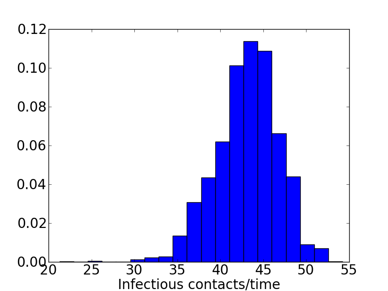
(b)

(c)

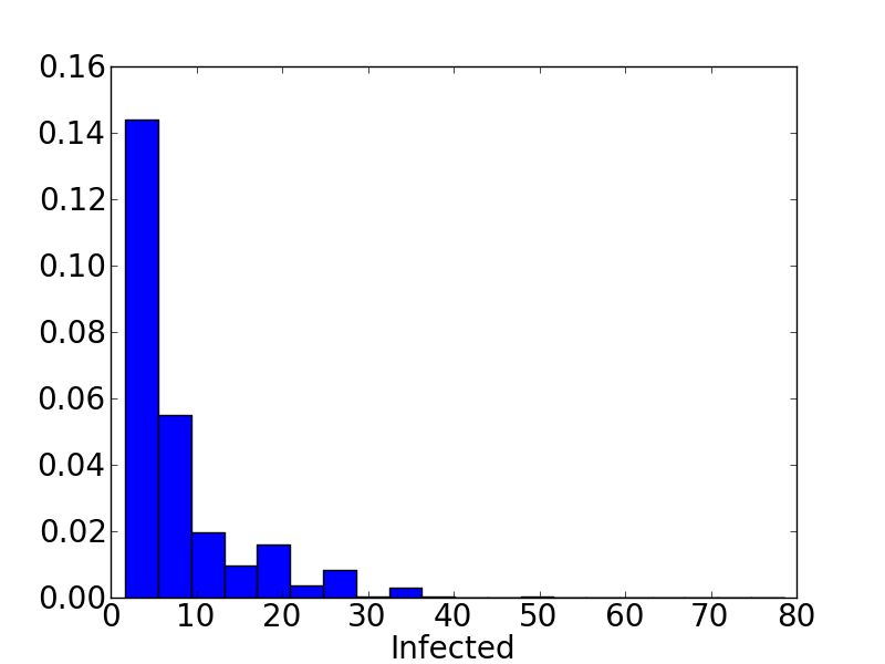
(d)

Figure 2: Synthetic data with $b_{0}=40,b_{1}=7$ and $N=200$, 14 observations trimmed away from the end. (a) True model (blue) and MAP estimated model (green), 5% and 95% quantile bands and box-plots for the posterior predictive distribution at two future points (actual data in *). Posterior distributions for $b_{0}$ (b), $b_{1}$ (c) and $R_{0}$ (d).

5 Example: Dengue Fever Outbreaks

There are numerous studies on the estimation of the basic reproductive number for Dengue. Many of these works look at the local initiation of the outbreak to estimate directly the basic reproductive number (e.g., Chowell, Diaz-Dueñas, Miller et al, [52]; Mendes-Luz, Torres-Codeco, Massad et al, [53]) or use a phenomenological approach to approximate its upper bound (Hsieh and Chen, [54]; Hsieh and Ma, [55]). Here we are able to estimate the basic reproduction number and the fate of the epidemic for the Dengue outbreaks in Acapulco, Mexico, in 2005 and Cuernavaca, Morelos in 2008 using a full differential equations model as explained earlier.

In Table 1 we list some estimates for the reproductive number for Dengue with their corresponding confidence intervals (when available) and for different cities. The reader is referred to the cited reference for further details. We have omitted those references whose estimations show very large variability.

Table 1: Reported data on the basic reproduction number for Dengue from several sources. Adapted from Hsieh and Chen [54]

Source	$R_{0}$ or range	Confidence interval 95%
Hsieh and Ma [55]	$2.23$	$(1.47,3.00)$
Hsieh and Chen [54]	$3.93-4.67$
Koopman et al [56]	$1.33-2.40$
Marques el al [57]	$1.6-2.4$
Khoa et al [58]	$1.25-1.75$
Chowell et al [52]	$3.09$	$(2.34-3.84)$
Chowell et al [52]	$2.0$	(1.75-2.23)
Chowell et al [59]	$1.76$
Massad et al [60]	$1.9$

In the 2005 and 2008 epidemic outbreaks recorded for the cities of Acapulco, state of Guerrero, and Cuernavaca, state of Morelos, Mexico, respectively only one viral strain was identified (no co-circulation of various serotypes). In 2005 DEN-1 and DEN-2 in Guerrero was isolated (Carrillo-Valenzo, Danis-Lozano, Velasco-Hernández et al, [61] and data from Dirección General de Epidemiología) and in 2008 in Morelos it was DEN-2 (Dirección General de Epidemiología)

By using the SIR model we are neglecting the role of the population dynamics of the mosquito during the epidemic outbreak and are, therefore, incorporating its effects as part of the constant contact rate $b_{1}$. Our rationale behind this assumption is the following: during the epidemic period the density of mosquito increases substantially. Smith, Dushoff and McKenzie [62] have shown that during an epidemic outbreak the human biting rate is highest shortly after mosquito density peaks and that the proportion of infected mosquitoes peaks when mosquito population density is declining. On the other hand Sanchez, Vanlerberghe, Alfonso et al [63] show data that confirms that mosquito abundance is strongly correlated with an epidemic. There have been reports for Rio de Janeiro, however (Honorio, Nogueira, Codeco et al, [64]), that have shown that the time of highest case incidence is not associated with a local increase of vector abundance, observation that can be caused by the movement patterns of the population. In this work we are looking at a geographical scale that comprises large metropolitan areas where the environment for transmission, during an epidemic, can be thought of as saturated with mosquito although at a local level (that of city district, block or house), it might not be the case. A high mosquito density also implies a high turnover rate of mosquito generations that result in a constant availability of female adult mosquitoes for disease transmission. This observations justify the treatment of a Dengue epidemic outbreak as if it were the epidemic outbreak in a directly transmitted disease. Of course, this hypothesis breaks down in the interepidemic period also known as the “endemic” state where low prevalence, asymptomatic infections and vector abundance are subject to stochastic environmental effects as well as to the seasonal forcing induced by the rainy season on the vector population. Consequently, we limit our estimation to the length of time of the epidemic outbreak in each one of the cases analyzed.

In summary we use the susceptible, infectious, recovered (SIR) Kermack McKendrick model as an approximation for the Dengue dynamics (e.g., Adams, Holmes, Zhang et al, [65]) for only one epidemic period. We therefore disregard demographic influences since births and deaths may be considered to have negligible effects on disease dynamics during this short time period and assume the mosquito population dynamics is constant and plays a role as a factor in the contact rate.

We rewrite now model (2)-(4) with the standard epidemiological notation where $b_{0}$ is the contact rate, $1/\gamma$ is the length of the infectious period and $N=y_{1}+y_{2}+y_{3}$ is the total population density:

$$\dot{y}_{1} =-b_{0}\frac{y_{2}}{N}y_{1}$$ (11)

$$\dot{y}_{2} =b_{0}\frac{y_{2}}{N}y_{1}-\gamma y_{2}$$ (12)

$$\dot{y}_{3} =\gamma y_{2}.$$ (13)

The basic reproduction number for this system is

$$R_{0}=\frac{b_{0}}{\gamma},$$

where we have rescaled the total population to be $N=1$. For comparison the simplest vector transmitted disease based on the Ross-Macdonald model renders a reproductive number of the form

$$R_{v}=\frac{abm}{\delta\gamma^{\prime}}$$

where $a$ and $b$ are the mosquito and human biting rates, $m$ is the ratio of female mosquitoes to human hosts and $1/\delta$ and $1/\gamma^{\prime}$ are the infectiousness periods for mosquito and human respectively.

It is obvious that the infection rate in the SIR model, $1/\gamma$, includes the total time available per capita for infection in both mosquito and human hosts; also the contact rate $b_{0}$ in the Kermack-McKendrick model aggregates the combined effect of the product $ab$ in $R_{v}$. Therefore the estimates of $R_{0}$ that we are about to obtain by applying our methods, will not discriminate the different components of this threshold parameter. Our methods, however, can be applied directly to more complicated models that explicitly incorporate the relevant parameters for the human and vector populations if necessary.

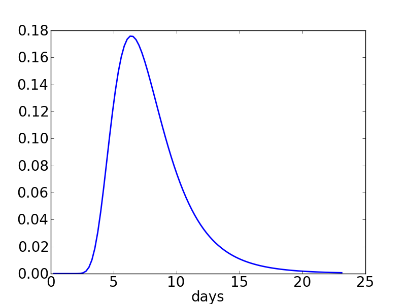
Figure 3: Inverse Gamma prior distribution for $\rho_{1}=1/\gamma=1/b_{1}$ for our Dengue outbreaks examples.

5.1 Acapulco 2005 and Cuernavaca 2008 outbreaks

Here we apply our methods to the two data sets described in section (3.3). For completeness we provide now a brief description of the basic life-cycle facts of the Dengue virus. The endemic-epidemic cycle of Dengue has the following characteristics. After an infected human host is bitten the viral incubation period within the mosquito lasts about 7-14 days after which the mosquito becomes infectious for its entire lifespan which is at most 25 days. In the human host the incubation period last form 3-14 days (with an average of 7). The infectious period lasts for about 2-10 days after outset of symptoms. Values on biting rates are not available and these are the main components that are estimated or circumvented when dealing with the basic reproduction number (see Chowell, Diaz-Dueñas, Miller et al, [52] and Hsieh and Chen, [54]). Since we do not have information for $\rho=1/b_{0}$ we use a uniform prior over a very long range (not shown). The prior information for the infectious period $\rho_{1}=1/b_{1}$ is shown in Figure 3. Recall that $\rho_{1}=1/\gamma$ is aggregating the infectious period of both the human host and vector discounted by the time allocated to viral incubation. To see this consider the following rough approximation: take the average human infectious period of 7, and the mosquito infectious period of about 10 days. The total time available for transmission is $7\times 10=70$; the proportion of the mosquito and human lifespan available to infection given the extrinsic and intrinsic incubation periods is the weighting factor that should be incorporated into $1/\gamma$. Suppose an extreme scenario where all the mosquito lifespan is infectious and that the human intrinsic incubation period is 10 days; then roughly the proportion of time available for closing a transmission cycle human-vector-human is $1\times 1/10=0.1$ which when multiplied by 70 gives the mode assigned to the prior for $\rho_{1}=1/\gamma$ shown in Figure  3. For this inverse gamma distribution for $\rho_{1}=1/\gamma=1/b_{1}$ the shape parameter is set to 9 and the scale parameter is 8 (9-1). Its mean is therefore 8 (days; these are in fact equal to $\alpha_{1}$ and $\beta_{1}$, given the shape and scale parametrization used for the Gamma prior for $b_{1}=\gamma$ in (10)).

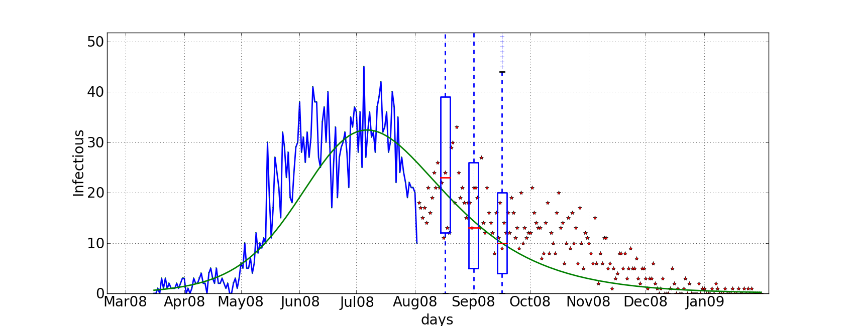
(a)

(b)

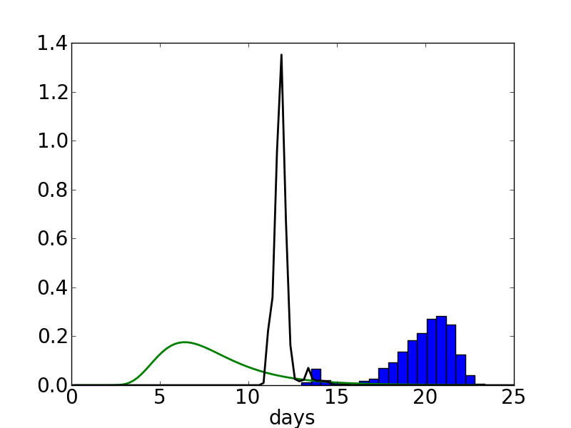
(c)

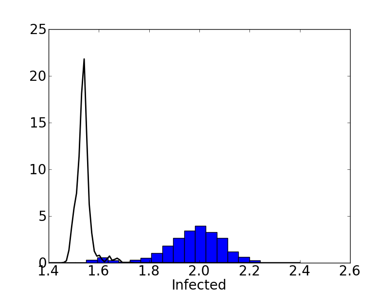
(d)

Figure 4: (a) Daily reported cases of Dengue fever in Cuernavaca, Mexico, 2008, with several observations trimmed away at the end. Estimated MAP model and three future fortnights of reported cases predicted (box-plots of predictive distribution), actual data with plotted with *. (b) Posterior distribution for $b_{0}$ (c) Posterior (histogram) and prior distribution for $\rho_{1}=1/b_{1}$ and (d) posterior distribution of $R_{0}=b_{0}/\gamma$. The approximated posterior densities with the full data are also presented (black).

For the Cuernavaca outbreak the MAP estimator of the reproductive number $R_{0}$ is 1.9 with $(1.8,2.2)$ as HPD 95% probability interval, when August to December 2008 are not considered in the estimation. The prediction of the fate of the epidemic is rather impressive, capturing basically all the data variability (see Figure 4). Intentionally, we chopped off data at the end of a descending fluctuation run, after the epidemic maximum, in early August 2008. The descending run did not fool our predictions of the future evolution of the epidemic (see the predictive distribution Box-Plots in Figure 4(a)). At that point, reasonable estimates for $b_{0}$ and $b_{1}$ were already available and good predictions could be done, taking into account all modeled sources of variability.

For the Acapulco outbreak the MAP estimator of the reproductive number $R_{0}$ is 1.3 with $(1.1,1.6)$ as HPD 95% probability interval when data starting in November 2005 are not considered in the estimation. The prediction of the fate of the epidemic is quite good considering the few data points used in the analysis (see Figure 5).

The estimate for Acapulco is in the lower range of values reported in Table 1. In fact, only the lower bound for the range in Khoa et al [58] is comparable in magnitude. The estimate for Cuernavaca is located more within the range reported by several studies.

We remark that the scarce (monthly) data from Acapulco leads to less informative predictions, hiding the intrinsic stochasticity of the state variables. In contrast data from Cuernavaca are reported weekly, See Figure 4. There are two possible explanations for this trend. Either, there might be two waves of Dengue, one starting in early April and other developing in early August 2008. The SIR model is unable to capture this dynamics in the local detail (late July-early August) but it is able to capture the tail of the epidemic outbreak reasonably well (see Figure 4a). If this hypothesis of two Dengue waves was true, the second wave of the epidemic corresponds may correspond to a different set of parameters, that increases the incidence immediately starting in August. On the other hand, the decreasing trend in August may be explained by demographic stochasticity alone.

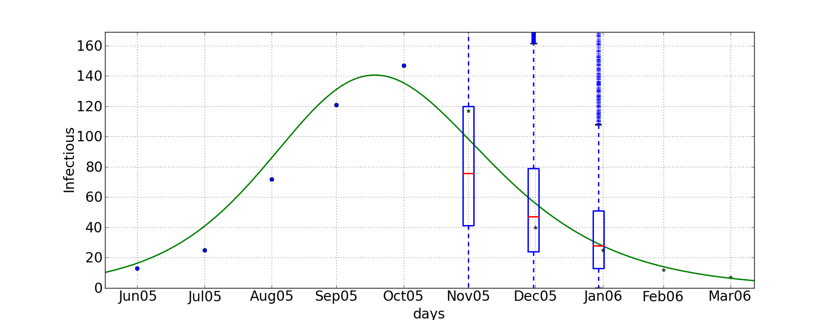
(a)

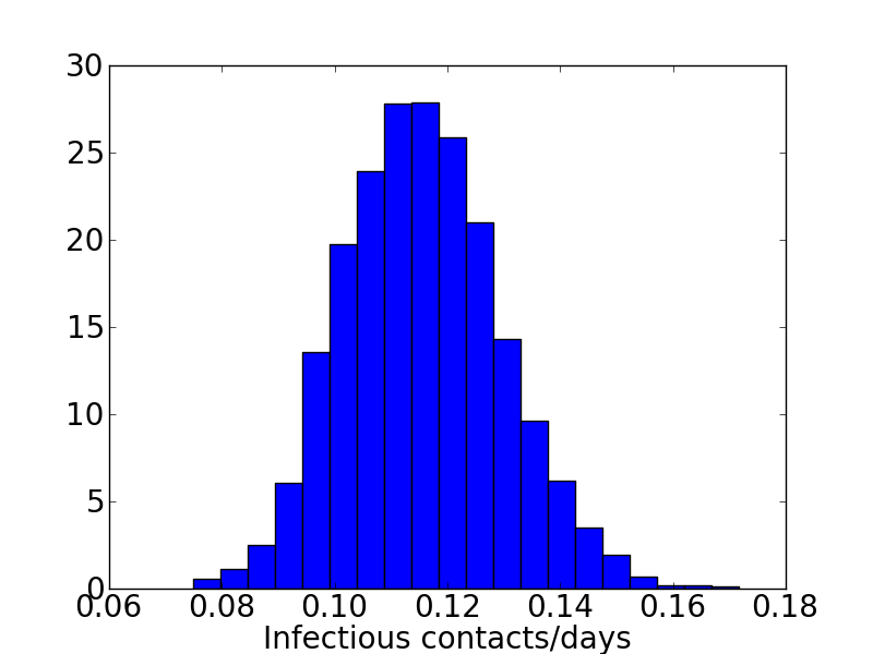
(b)

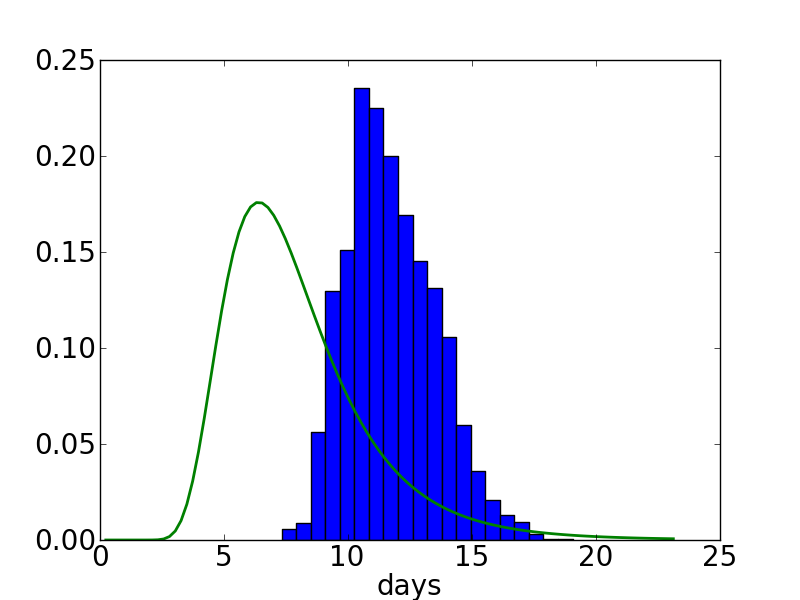
(c)

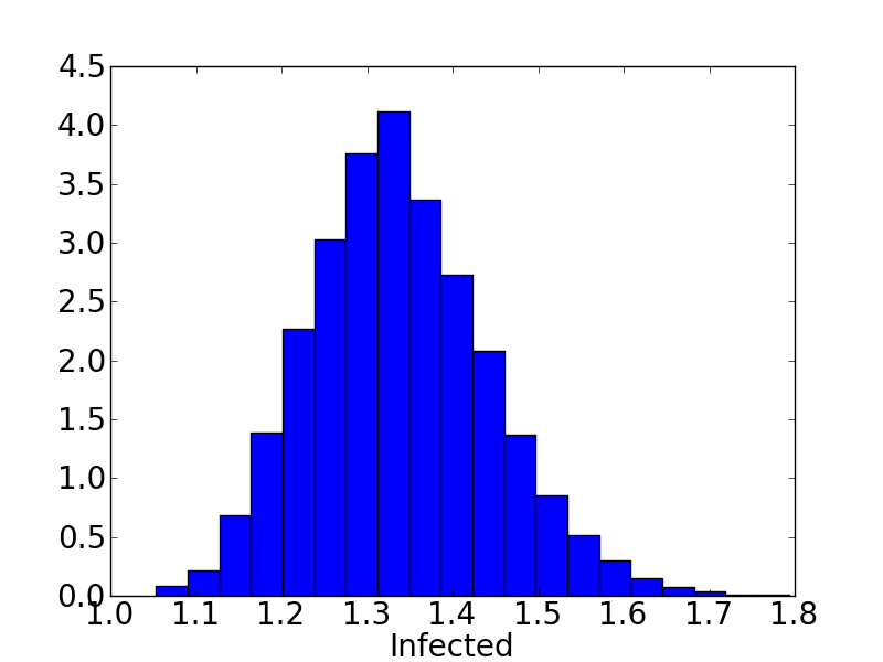
(d)

Figure 5: Reported cases of Dengue fever in Acapulco, Mexico, 2005, with 6 observations trimmed away at the end. Estimated MAP model and three future months of reported cases predicted (box-plots of predictive distribution), actual data plotted with *. (b) Posterior (histogram) and prior distribution for $\rho_{0}=1/b_{0}$. (c) Posterior (histogram) and prior distribution for $\rho_{1}=1/b_{1}$ and (d) posterior distribution of $R_{0}=b_{0}/\gamma$.

6 Conclusions

With respect to this approach as an useful inferential and predictive framework for epidemic surveillance data, Breban, Vardavas and Blower [66] present a critique to estimating $R_{0}$ using population level models. These authors claim that using an individual-level model approach to estimate $R_{0}$ is more accurate and may not coincide with the $R_{0}$ estimated from a population level model. In the approach we present here, the incorporation of the CME formalism introduces demographic stochasticity, i.e., individual stochastic variation into the epidemic parameters $b_{0}$ and $b_{1}$ thus actually approximating individual level characteristics. The methods shown here do generate distributions of the basic parameters, including $R_{0}$ based on the a priori information available. To reinforce our point the results by Lloyd-Smith, Schreiber, Kopp and Getz [67] show that $R_{0}$ has an highly skewed distribution in many diseases when sampled from individuals through contact-tracing. Certainly our results Figures (4) and (5) do show (admittedly only slightly) skewed distributions that indicates the individual variability in contact and recovery rates at the individual level. This variability does not come from sampling errors but from an intrinsic property of stochastic individual variation constructed into the model via the CME. Our estimation approach uses this built-in demographic stochasticity to estimate $R_{0}$. We are using a very simple model, the SIR without vital dynamics and this may explain the relatively low variability reflected in our nearly symmetric distributions: the model is smoothing out individual differences. We are using the simplest priors that are biologically reasonable.

In general, we expect to generate highly skewed distributions for at least one of our parameters when, for example, few data points are available and the uncertainty in estimating $b_{1}$ is such that its posterior distribution borders on zero, the distribution of $R_{0}=b_{0}/b_{1}$ will result heavily skew with a long tail (as in Figure 2(d)).

Indeed, the SIR model presented here is quite simple, and specially applied to (vector induced, delayed, etc.) Dengue. Nevertheless, we obtained interesting inferences and prediction power from limited data, in real and synthetic scenarios, and the model simplicity servers us to present and experiment with our inference procedure. Our inference framework can indeed be generalized to be used in a more complex model (as explained in Section 2), were for example the vector-human interaction is modeled in a more comprehensive way. We leave this for further research.

7 Acknowledgments

We thank the support, expert commentaries and insight into the complex dynamics of Dengue fever of José Ramos-Castañeda, Ruth Aralí Martínez-Vega and Rogelio Danis-Lozano who also provided the the data on Dengue that we have used here. We also acknowledge the very fruitful discussions with the network on Biology and Ecology from CONACyT’s Red en Modelos Matemáticos y Computacionales. JXVH acknowledges partial funding from the National Institute for Mathematical and Biological Synthesis through the National Science Foundation EF-0832-858.

References

- [1] D. Alonso, A. McKane, M. Pascual, Stochastic amplification in epidemics, Journal of the Royal Society Interface 4 (14) (2007) 575.
- [2] A. King, E. Ionides, M. Pascual, M. Bouma, Inapparent infections and cholera dynamics, Nature 454 (7206) (2008) 877–880.
- [3] L. Shaw, I. Schwartz, Fluctuating epidemics on adaptive networks, Physical Review E 77 (6) (2008) 66101.
- [4] I. Nåsell, Stochastic models of some endemic infections, Mathematical Biosciences 179 (1) (2002) 1–19.
- [5] W. Chen, S. Bokka, Stochastic modeling of nonlinear epidemiology, Journal of theoretical biology 234 (4) (2005) 455–470.
- [6] A. Black, A. McKane, Stochastic amplification in an epidemic model with seasonal forcing, Journal of Theoretical Biology.
- [7] H. Qian, Nonlinear stochastic dynamics of mesoscopic homogeneous biochemical reaction systems—an analytical theory, Nonlinearity 24 (2011) R19.
- [8] O. Björnstad, B. Finkenstädt, B. Grenfell, Dynamics of measles epidemics: estimating scaling of transmission rates using a time series SIR model, Ecological Monographs 72 (2) (2002) 169–184.
- [9] C. Gilligan, S. Gubbins, S. Simons, Analysis and fitting of an SIR model with host response to infection load for a plant disease, Philosophical Transactions of the Royal Society B: Biological Sciences 352 (1351) (1997) 353.
- [10] Y. Kuznetsov, C. Piccardi, Bifurcation analysis of periodic SEIR and SIR epidemic models, Journal of mathematical biology 32 (2) (1994) 109–121.
- [11] P. Van den Driessche, J. Watmough, A simple SIS epidemic model with a backward bifurcation, Journal of Mathematical Biology 40 (6) (2000) 525–540.
- [12] C. Kribs-Zaleta, J. Velasco-Hernandez, A simple vaccination model with multiple steady-states, Mathematical Biosciences 164 (2000) 183–201.
- [13] M. Alexander, S. Moghadas, Periodicity in an epidemic model with a generalized non-linear incidence, Mathematical biosciences 189 (1) (2004) 75–96.
- [14] P. Rohani, M. Keeling, B. Grenfell, The interplay between determinism and stochasticity in childhood diseases, American Naturalist 159 (5) (2002) 469–481.
- [15] J. Dushoff, J. Plotkin, S. Levin, D. Earn, Dynamical resonance can account for seasonality of influenza epidemics, Proceedings of the National Academy of Sciences of the United States of America 101 (48) (2004) 16915.
- [16] B. Finkenstädt, O. Björnstad, B. Grenfell, A stochastic model for extinction and recurrence of epidemics: estimation and inference for measles outbreaks, Biostatistics 3 (4) (2002) 493.
- [17] H. Andersson, T. Britton, Stochastic epidemic models and their statistical analysis, Springer Verlag, 2000.
- [18] J. Ramsay, G. Hooker, D. Campbell, J. Cao, Parameter estimation for differential equations: a generalized smoothing approach, Journal of the Royal Statistical Society: Series B (Statistical Methodology) 69 (5) (2007) 741–796.
- [19] B. Munsky, B. Trinh, M. Khammash, Listening to the noise: random fluctuations reveal gene network parameters, Molecular systems biology 5 (1).
- [20] C. Archambeau, M. Opper, Approximate inference for continuous-time markov processes, Inference and Estimation in Probabilistic Time-Series Models. Cambridge University Presse.
- [21] G. Rempala, K. Ramos, T. Kalbfleisch, A stochastic model of gene transcription: an application to l1 retrotransposition events, Journal of Theoretical Biolology 242 (1) (2006) 101–116.
- [22] A. Golightly, D. Wilkinson, Bayesian sequential inference for stochastic kinetic biochemical network models, Journal of Computationl Biology 13 (3) (2006) 838–851.
- [23] T. Tian, S. Xu, J. Gao, K. Burrage, Simulated maximum likelihood method for estimating kinetic rates in gene expression, Bioinformatics 23 (2007) 84–91.
- [24] A. Golightly, D. Wilkinson, Bayesian inference for stochastic kinetic models using a diffusion approximation, Biometrics 61 (3) (2005) 781–788.
- [25] M. Komorowski, B. Finkenstädt, C. Harper, D. Rand, Bayesian inference of biochemical kinetic parameters using the linear noise approximation, BMC bioinformatics 10 (1) (2009) 343.
- [26] A. Ruttor, G. Sanguinetti, M. Opper, Approximate inference for stochastic reaction processes., in: N. Lawrence, M. Girolami, M. Rattray, G. Sanguinetti (Eds.), Learning and Inference in Computational Systems Biology, MIT Press, 2009, Ch. 11, pp. 277–296.
- [27] A. Ruttor, M. Opper, Efficient statistical inference for stochastic reaction processes, Physical review letters 103 (23) (2009) 230601.
-
[28]
J. Marin, P. Pudlo, C. P. Robert, R. Ryder,
Approximate
Bayesian Computational methods, Tech. rep.,
http://adsabs.harvard.edu/abs/2011arXiv1101.0955M (2011).
arXiv:1101.0955.
URL http://adsabs.harvard.edu/abs/2011arXiv1101.0955M - [29] T. Toni, D. Welch, N. Strelkowa, A. Ipsen, M. Stumpf, Approximate bayesian computation scheme for parameter inference and model selection in dynamical systems, Journal of the Royal Society Interface 6 (31) (2009) 187.
-
[30]
C. Robert, J. Marin, N. Pillai, Why
approximate bayesian computational (abc) methods cannot handle model choice
problems, Tech. rep., http://arxiv.org/abs/1101.5091v2 (2011).
URL http://arxiv.org/abs/1101.5091v2 - [31] C. Gillespie, A. Golightly, Bayesian inference for generalized stochastic population growth models with application to aphids, Journal of the Royal Statistical Society Series C Applied Statistics 59 (2010) 341–357.
- [32] R. Boys, D. Wilkinson, T. Kirkwood, Bayesian inference for a discretely observed stochastic kinetic model, Statistics and Computing 18 (2008) 125–135.
- [33] C. Gardiner, Handbook of stochastic methods, Springer Berlin, 1985.
- [34] D. Gillespie, Stochastic simulation of chemical kinetics, Annual review of physical chemistry 58 (1) (2007) 35–55.
- [35] T. Turner, S. Schnell, K. Burrage, Stochastic approaches for modelling in vivo reactions, Computational Biology and Chemistry 28 (3) (2004) 165–178.
- [36] J. Pearson, P. Krapivsky, A. Perelson, Stochastic theory of early viral infection: Continuous versus burst production of virions, PLoS Computational Biology 7 (2) (2011) e1001058.
- [37] M. Kot, Elements of mathematical ecology, Cambridge Univ Pr, 2001.
- [38] W. Kermack, A. McKendrick, Contributions to the mathematical theory of epidemics I, Proceedings of the Royal Society 115A (1927) 700–721.
- [39] W. Kermack, A. McKendrick, Contributions to the mathematical theory of epidemics II. The problem of endemicity, Proceedings of the Royal Society 138A (1932) 55–83.
- [40] W. Kermack, A. McKendrick, Contributions to the mathematical theory of epidemics III. Further studies of the problem of endemicity, Proceedings of the Royal Society 141A (1933) 94–122.
- [41] D. Daley, J. Gani, Epidemic modelling: an introduction, Studies in Mathematical Biology, Cambridge University Press, Cambridge UK, 1999.
- [42] N. van Kampen, Stochastic processes in physics and chemistry, North Holland, 1992.
- [43] R. Kress, W. Rundell, A quasi-Newton method in inverse obstacle scattering, Inverse Problems 10 (1994) 1145.
- [44] S. Reinker, R. Altman, J. Timmer, Parameter estimation in stochastic biochemical reactions, IEE Systems Biology 153 (4) (2006) 168–178.
- [45] C. Gillespie, Moment-closure approximations for mass-action models, Systems Biology, IET 3 (1) (2009) 52–58.
- [46] M. Capistrán, J. Christen, A generic multivariate distribution for counting data, Arxiv preprint arXiv:1103.4866.
- [47] J. Liu, Monte Carlo Strategies in Scientific Computing, Series in Statistics, Springer, New York, 2001.
-
[48]
J. Christen, C. Fox,
A
general purpose sampling algorithm for continuous distributions (the
t-walk), Bayesian Analysis 5 (2) (2010) 263–282.
URL http://ba.stat.cmu.edu/journal/2010/vol05/issue02/chris%ten.pdf - [49] O. Diekmann, J. Heesterbeek, Mathematical epidemiology of infectious diseases: model building, analysis, and interpretation, Wiley, 2000.
- [50] J. M. Bernardo, A. F. M. Smith, Bayesian Theory, Wiley and Sons, Chichester, 1994.
- [51] F. C. Coelho, C. T. Codeco, M. G. M. Gomes, A bayesian framework for parameter estimation in dynamical models, PLoS ONE 6 (5) (2011) e19616. doi:10.1371/journal.pone.0019616.
- [52] G. Chowell, P. Diaz-Dueñas, J. Miller, et al., Estimation of the reproduction number of dengue fever from spatial epidemic data, Mathematical Biosciences 68 (2007) 571–589.
- [53] P. Mendes-Luz, C. Torres-Codeco, E. Massad, C. J. Struchiner, Uncertainities regarding Dengue modeling in Rio de Janeiro, Brazil, Memorias do Instituto Oswaldo Cruz 98 (7) (2003) 87–878.
- [54] Y. Hsieh, C. Chen, Turning points, reproduction number, and impact of climatological events for multi-wave dengue outbreaks, Tropical Medicine and International Health 14 (6) (2009) 628–638.
- [55] Y. Hsieh, S. Ma, Intervention measures, turning point, and reproduction number for dengue, Singapore, 2005, American Journal of Tropical Medicine and Hygiene 80 (1) (2009) 66–71.
- [56] J. Koopman, D. Prevots, M. Chao, et al, Determinant and predictors of dengue infection in Mexico, American Journal of Epidemiology 133 (1991) 1168–1178.
- [57] C. Marques, O. Foratini, E. Massad, The basic reproduction number for dengue fever in Sao Paulo State, Brazil: 1990-1991 epidemic, Transactions of the Royal Society of Tropical Medicine and Hygiene 88 (88–89).
- [58] T. Khoa, Q. Tran, T. Phan, et al., Seroprevalence of dengue antibodies, annual incidence and risk factors among children in southern Vietnam, Tropical Medicine and International Health 10 (2005) 379–386.
- [59] G. Chowell, C. Torre, C. Munayco-Escate, et al, Spatial and temporal dynamics of dengue fever in Peru, Epidemiological Infections 136 (1667–1677).
- [60] E. Massad, S. Ma, M. Burattini, et al., The risk of chikungunya fever in a dengue endemic area, Journal of Travel Medicine 15 (2008) 147–155.
- [61] E. Carrillo-Valenzo, R. Dans-Lozano, J. Velasco-Hernández, et al., Evolution of dengue virus in Mexico is characterized by frequent lineage replacements, Archives of Virology x (x) (2010) x.
- [62] D. L. Smith, J. Dushoff, F. E. McKenzie, The risk of a mosquito-borne infection in an heterogeneous environment, Plos Biology 2 (11) (2004) 1957–1964.
- [63] L. Sanchez, V. Vanlerberghe, L. Alfonso, et al., Aedes aegypti larval indices and risk for dengue epidemics., Emerging Infectious Diseases 12 (5) (2006) 800–806.
- [64] H. N.A., N. R.M, C. C.T., et al., Spatial evaluation and modeling of Dengue seroprevalence and vector density in Rio de Janeiro, Brazil, PLoS Neglegted Tropical Diseases 3 (11) (2009) e545.
- [65] B. Adams, E. C. Holmes, C. Zhang, et al., Cross-protective immunity can account for the alternating epidemic pattern of dengue virus serotypes circulating in Bangkok, Proceedings of the National Academy of Science, USA 103 (2006) 14234–14239.
- [66] R. Breban, R. Vardavas, S. Blower, Theory versus Data: How to calculate ?, Plos One 3 (282) (2007) 1–4.
- [67] J. Lloyd-Smith, S. Scheiber, P. Kopp, W. Getz, Superspreading and the effect of individual variation on disease emergence, Nature 438 (17) (2005) 355–359.