Transport through a quantum spin Hall quantum dot

Abstract

Quantum spin Hall insulators, recently realized in HgTe/(Hg,Cd)Te quantum wells, support topologically protected, linearly dispersing edge states with spin-momentum locking. A local magnetic exchange field can open a gap for the edge states. A quantum-dot structure consisting of two such magnetic tunneling barriers is proposed and the charge transport through this device is analyzed. The effects of a finite bias voltage beyond linear response, of a gate voltage, and of the charging energy in the quantum dot are studied within a combination of Green-function and master-equation approaches. Among other results, a partial recurrence of non-interacting behavior is found for strong interactions, and the possibility of controlling the edge magnetization by a locally applied gate voltage is proposed.

I Introduction

Topological insulators and superconductorsHaK10 ; RSF10 ; QiZ11 have recently become the topic of extensive experimental and theoretical research. These materials can be described in terms of weakly interacting quasiparticles and their single-particle Hamiltonians show non-trivial topological properties in momentum space. They have an energy gap in the bulk but a topologically protected gapless spectrum of boundary states. Schnyder et al.SRF08 ; RSF10 and KitaevKit09 have put forward an exhaustive classification of these systems in terms of their Altland-Zirnbauer symmetry classesZir96 and of the number of spatial dimensions.

A topologically nontrivial state is possible for the symplectic class AII in two dimensions, corresponding to systems with spin-orbit coupling in the absense of an applied magnetic field and of superconductivity. This so-called quantum spin Hall (QSH) stateMNZ03 ; SCN04 has protected edge states with gapless Weyl-type dispersion. Bernevig et al.BHZ06 have predicted and König et al.KWB07 ; KBM08 have observed the QSH effect in HgTe/(Hg,Cd)Te quantum wells.

The edge states of the QSH system show spin-momentum locking in the sense that right-moving (left-moving) electrons are strictly spin-up (spin-down).HaK10 ; QiZ11 ; KBM08 Consequently, density-density interactions cannot lead to backscattering since they cannot flip the spin. On the other hand, spin-dependent scattering, for example by magnetic impurities, can lead to backscattering. Unconventional transport properties are thus expected and possible applications in spintronics can be envisaged. It is therefore of interest to study electronic transport in prototypical device geometries involving QSH edge states, which is the subject of this paper.

The underlying idea is to realize a quantum dot as a finite-length segment of a QSH edge. This cannot be achieved by electrostatic gating since an electric potential just shifts the edge bands up or down without opening a gap and thus does not lead to the formation of tunneling barriers. However, such barriers could be realized by ferromagnetic insulators grown in contact with the edge. They would impose an exchange magnetic field orthogonal to the spin-orbit field and open a gap. We also include a gate electrode that can be used to tune the electrostatic potential on the quantum dot. Figure 1 shows a sketch of the device. Since the QSH edge states typically have a small Fermi wavenumber $k_{F}$, we consider the case that the barrier width is negligible compared to $\lambda_{F}=2\pi/k_{F}$. We restrict ourselves to the cases of parallel and antiparallel exchange fields in the two barriers. Finally, we assume the thermal energy $k_{B}T$ to be small compared to the lifetime broadening of the dot levels so that we can set the temperature to zero. Including a finite temperature is straightforward. An alternative realization of a QSH quantum dot as the edge of a small QSH puddle has been analyzed by Tkachov and Hankiewicz,TkH11 for negligible charging energy. They have also studied contributions to the resistance due to the coupling of a QSH edge to normal leads and the effect of an orbital magnetic field parallel to the spin-orbit field.TkH11

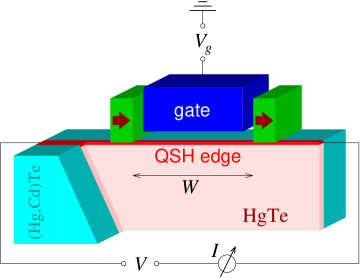
Figure 1: (Color online) Cut-away view of the QSH quantum dot.

After introducing the model in Sec. II, we study the effect of the gate voltage and the bias voltage on the transport in Sec. III. A Landauer approachLan57 is used to obtain the current for arbitrary strength of the magnetic barriers. We will see that the result can also be analyzed in terms of a generalized Meir-Wingreen (MW) formula for the currentMeW92 ; JWM94 in terms of the non-interacting Green function. It is generalized in the sense of pertaining to a real-space continuum Hamiltonian instead of a tunneling Hamiltonian, which leads to a nontrivial form of the dot-lead coupling functions $\Gamma^{L}$, $\Gamma^{R}$.

In the next step, the effect of electron-electron interaction on the dot is studied in Sec. IV. We again employ a simple model by including a charging energy in terms of the excess charge. This is valid if the range of the electron-electron interaction is large compared to the dot size $W$, i.e., for small dots, but should give qualitatively correct results beyond this regime. The opposite case of short-range interactions is certainly of interest. For an unmodulated QSH edge this case has been studied for example in Refs. WBZ06, , XuM06, , BDR11, . A quantum dot in a spinless Luttinger liquid, not a QSH edge, has been studied by several authors.KaF92 ; FuN93 ; ChW93 ; MEA05 Tunneling through a quantum dot between two QSH edges described as Luttinger liquids has been addressed by Law et al.LSL10

In Sec. IV, we employ an equation-of-motion approach to obtain the multiple-pole structure of the spectral function appearing in the generalized MW formula. We discuss possible approximations for the weights of the poles and show results calculated from a master equation in the sequential-tunneling approximation with additional level broadening, valid for weak coupling through the magnetic barriers. We summarize the main results in Sec. V.

II Model

The non-interacting part of the Hamiltonian of the QSH edge with magnetic barriers is written as a $2\times 2$ matrix in spin space,

$$H_{0} = -i\hbar v_{F}\sigma^{z}\partial_{x}-\eta\hbar v_{F}\sigma^{x}\delta(x)\mp\eta\hbar v_{F}\sigma^{x}\delta(x-W)$$ (1)

$${}+V(x),$$

where $v_{F}$ is the Fermi velocity, $\sigma^{x}$ and $\sigma^{z}$ are Pauli matrices, $\eta$ is the dimensionless strength of the magnetic barriers, and $V(x)$ is a non-uniform electric potential. A $2\times 2$ unit matrix is implied in the last term. $H_{0}$ is certainly only valid within the bulk energy gap. The first term is the Weyl Hamiltonian of the bare edge.KBM08 ; VaO11 We neglect higher-order spatial derivatives, which lead to non-linear terms in the dispersion. An electric field perpendicular to the layers induces an additional Rashba spin-orbit-coupling term $H_{R}=-i\alpha\sigma^{y}\partial_{x}$. However, this term can be absorbed into the Weyl term by a rotation in spin space.VaO11 The upper (lower) sign of the third term refers to parallel (antiparallel) exchange fields in the two barriers. The parameter $\eta$ can be written as

$$\eta=\frac{g\mu_{B}B_{\mathrm{exc}}L}{\hbar v_{F}},$$ (2)

where $g$ is the g-factor, $\mu_{B}$ is the Bohr magneton, $B_{\mathrm{exc}}$ is the exchange field, and $L$ is the width of the magnetic barrier. Equation (1) is obtained in the limit $B_{\mathrm{exc}}\to\infty$, $L\to 0$, keeping $B_{\mathrm{exc}}L$ constant. For the potential $V(x)$ we take

$$V(x)=\left\{\begin{array}[]{ll}eV/2&\mbox{for $x\leq 0$},\\[2.15277pt] -eV_{g}&\mbox{for $0<x\leq W$},\\[2.15277pt] -eV/2&\mbox{for $x>W$},\end{array}\right.$$ (3)

where $V$ is the bias voltage and $V_{g}$ is the gate voltage.

Since the time-independent Schrödinger equation resulting from $H_{0}$ is of first order in spatial derivatives, we can solve it by means of a (non-unitary) “spatial-evolution operator.” Multiplying the Schrödinger equation by $\sigma^{z}$ from the left, we obtain

$$\partial_{x}\psi = i\,\frac{E-V(x)}{\hbar v_{F}}\,\sigma^{z}\,\psi(x)$$ (4)

$${}-\eta\,\sigma^{y}\,\delta(x)\,\psi(x)\mp\eta\,\sigma^{y}\,\delta(x-W)\,\psi(x),$$

which for $x\geq x_{0}$ is solved by

$$\psi(x) = S_{\leftarrow}\,\exp\bigg{(}\int_{x_{0}}^{x}dx^{\prime}\,\bigg{[}i\,\frac{E-V(x^{\prime})}{\hbar v_{F}}\,\sigma^{z}$$ (5)

$${}-\eta\,\sigma^{y}\,\delta(x^{\prime})\mp\eta\,\sigma^{y}\,\delta(x^{\prime}-W)\bigg{]}\bigg{)}\,\psi(x_{0}),$$

where $S_{\leftarrow}$ is a spatial-ordering directive; operators acting on $\psi(x_{0})$ are ordered with their spatial coordinates increasing from right to left. We can obtain the boundary condition at the barrier at $x=0$ by making $x_{0}$ infinitesimally negative and $x$ infinitesimally positive,

$$\psi(0^{+})=e^{-\eta\sigma^{y}}\,\psi(0^{-})=(\cosh\eta-\sigma^{y}\sinh\eta)\,\psi(0^{-}).$$ (6)

Since the Schrödinger equation is of first order in spatial derivatives, there is only a single boundary condition.footnote.BC Analogously, we find the boundary condition at the other barrier, $\psi(W^{+})=(\cosh\eta\mp\sigma^{y}\sinh\eta)\,\psi(W^{-})$.

To study transport, we assume the states in the leads to be filled up to the chemical potential $\mu$, measured relative to the Weyl nodes (band crossing points), which are shifted by the potential $\pm eV/2$. We take $\mu$ to be the same in the two leads since they are parts of the edge of the same quantum well.

In the following, we will need the eigenstates of the decoupled dot, which corresponds to the limit $\eta\to\infty$. The solution is straightforward: The Schrödinger equation for the eigenspinors $\psi_{\nu}(x)$ to eigenenergies $E_{\nu}$ reads

$$-i\hbar v_{F}\sigma^{z}\,\partial_{x}\psi_{\nu}-eV_{g}\,\psi_{\nu}(x)=E_{\nu}\,\psi_{\nu}(x)$$ (7)

with the boundary conditions

$$(1+\sigma^{y})\,\psi_{\nu}(0)=0,\qquad(1\mp\sigma^{y})\,\psi_{\nu}(W)=0,$$ (8)

which give

$$\psi_{\nu\downarrow}(0)=-i\,\psi_{\nu\uparrow}(0),\qquad\psi_{\nu\downarrow}(W)=\pm i\,\psi_{\nu\uparrow}(W).$$ (9)

The normalized solutions are

$$\psi_{\nu}(x)=\frac{1}{\sqrt{2W}}\left(\begin{array}[]{c}\exp\left(i\,\frac{E_{\nu}+eV_{g}}{\hbar v_{F}}\,x\right)\\[6.45831pt] -i\,\exp\left(-i\,\frac{E_{\nu}+eV_{g}}{\hbar v_{F}}\,x\right)\end{array}\right)$$ (10)

with

$$E_{\nu}=-eV_{g}+\frac{\pi\hbar v_{F}}{W}$$ (13)

$${}\times\left\{\begin{array}[]{ll}\nu+1/2&\mbox{for parallel exchange fields},\\ \nu&\mbox{for antiparallel exchange fields},\end{array}\right.$$

where $\nu$ can assume any integer value. Note that the spectrum is an equidistant ladder, which is, unlike for the harmonic oscillator, unbounded from both above and below. The level spacing is $E_{0}:=\pi\hbar v_{F}/W$. Of course, the discrete spectrum only exists inside the bulk gap and is only equidistant as long as non-linear terms in the dispersion of the edge states can be neglected. In the absense of a gate voltage, the spectrum is symmetric with respect to zero energy for both orientations of the exchange fields due to the particle-hole symmetry of $H_{0}$. For antiparallel exchange fields, one eigenstate has energy zero.

Finally, the Coulomb interaction is described by the particle-hole-symmetric term $H_{\mathrm{int}}=({e^{2}}/{2C})\,(\Delta n)^{2}$, where $C$ is the capacitance of the quantum dot and $\Delta n$ is the excess number of electrons on the dot compared to neutrality. In terms of the number operators $n_{\nu}=c_{\nu}^{\dagger}c_{\nu}$ of single-particle dot states $|\nu\rangle$, we have

$$H_{\mathrm{int}}=\frac{e^{2}}{2C}\,\bigg{[}\sum_{\nu}\bigg{(}n_{\nu}-\frac{1}{2}\bigg{)}\bigg{]}^{2}.$$ (14)

III Transport through a non-interacting dot

Neglecting the electron-electron interaction, the current through the QSH quantum dot can be expressed in terms of its transmission coefficient $T(E)$ by the Landauer formula,Lan57

$$I=\frac{e}{h}\,\int_{\mu-eV/2}^{\mu+eV/2}dE\>T(E).$$ (15)

Since $T(E)$ does no depend on the bias voltage $V$ in our case, the differential conductance is simply given by

$$\frac{dI}{dV}=\frac{e^{2}}{h}\,\frac{T(\mu+eV/2)+T(\mu-eV/2)}{2}.$$ (16)

The transmission coefficient $T(E)$ is obtained from the transfer matrix $\mathcal{T}=\mathcal{T}_{R}\mathcal{T}_{\mathrm{dot}}\mathcal{T}_{L}$ of the device, where the three factors are the transfer matrices of the right barrier, the dot region, and the left barrier, respectively. Since the right-moving (left-moving) electrons have spin up (down), Eq. (6) implies that the transfer matrix for the left barrier is

$$\mathcal{T}_{L}=\cosh\eta-\sigma^{y}\sinh\eta=\left(\begin{array}[]{cc}\cosh\eta&i\,\sinh\eta\\ -i\,\sinh\eta&\cosh\eta\end{array}\right).$$ (17)

(The transmission coefficient of a single barrier thus equals $1/\cosh^{2}\eta$.) For the right barrier we get

$$\mathcal{T}_{R}=\left(\begin{array}[]{cc}\cosh\eta&\pm i\,\sinh\eta\\ \mp i\,\sinh\eta&\cosh\eta\end{array}\right).$$ (18)

The transfer matrix for the dot region can be infered from the spatial-evolution operator in Eq. (5) for $x_{0}=0^{+}$, $x=W^{-}$,

$$\mathcal{T}_{\mathrm{dot}}=\exp\left(i\,\frac{E+eV_{g}}{\hbar v_{F}}\,\sigma^{z}W\right)$$ (21)

$$=\left(\begin{array}[]{cc}\exp\left(i\,\frac{E+eV_{g}}{\hbar v_{F}}\,W\right)&0\\ 0&\exp\left(-i\,\frac{E+eV_{g}}{\hbar v_{F}}\,W\right)\end{array}\right).\quad$$

The transmission coefficient $T=|t|^{2}$ is obtained in the standard way by solving

$$\mathcal{T}_{R}\mathcal{T}_{\mathrm{dot}}\mathcal{T}_{L}\,\left(\begin{array}[]{c}1\\ r\end{array}\right)=\left(\begin{array}[]{c}t\\ 0\end{array}\right)$$ (22)

for $t$. The result is

$$T(E)=\frac{1}{1+\mathop{\mathrm{trg}}^{2}\left(\frac{E+eV_{g}}{\hbar v_{F}}\,W\right)\,\sinh^{2}2\eta},$$ (23)

where $\mathop{\mathrm{trg}}=\cos$ ($\sin$) for parallel (antiparallel) exchange fields. The transmission is maximal whenever the energy $E$ coincides with an eigenenergy $E_{\nu}$ of the decoupled dot. In this situation, the transmission coefficient is unity so that the device is perfectly transparent on resonance. The width of the maxima is controlled by the strength of the magnetic barriers, $\eta$, with the width getting exponentially small for large $\eta$. This is more easily seen by writing the transmission coefficient as a series,

$$T(E)=\frac{E_{0}}{2\pi\,\cosh 2\eta}\sum_{\nu=-\infty}^{\infty}\frac{2\gamma}{(E-E_{\nu})^{2}+\gamma^{2}},$$ (24)

where the width of the Lorentzian peaks is

$$\gamma:=\frac{E_{0}}{\pi}\,\ln\coth\eta.$$ (25)

An analytical expression for the current can be obtained by inserting $T(E)$ into Eq. (15). We defer this to the next section.

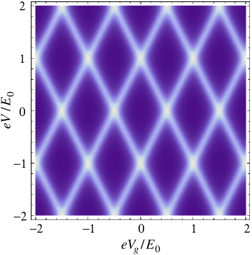
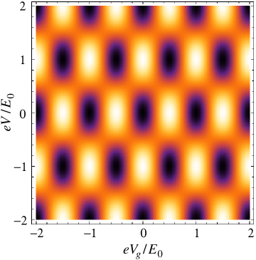
(a) (b) (c)

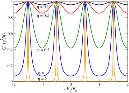
Figure 2: (Color online) Density plots of the differential conductance $dI/dV$ through a QSH quantum dot with parallel exchange fields as a function of gate voltage $V_{g}$ and bias voltage $V$ in the absence of electron-electron interaction. The dimensionless strength of the magnetic barriers was set to (a) $\eta=1$ and (b) $\eta=0.1$, respectively. Light colors denote large $dI/dV$. (c) Linear conductance $G=dI/dV|_{V=0}$ as a function of the gate voltage $V_{g}$. The level spacing of the decoupled dot, $E_{0}=\pi\hbar v_{F}/W$, is used as the energy unit.

This is not required for deriving the differential conductance $dI/dV$, which can immediately be read off from Eqs. (16) and (23). Note that the chemical potential $\mu$ and the gate voltage $V_{g}$ only appear in the combination $eV_{g}+\mu$ since only energy differences between the dot and the leads enter. We can thus set $\mu=0$ without loss of generality. $dI/dV$ is plotted in Fig. 2 as a function of gate and bias voltages. The figure clearly exhibits the suppression of the low-bias conductance off resonance due to Pauli blockade. The Pauli-blockade diamonds are filled in for strong coupling to the leads (weak magnetic barriers), and for $\eta\to 0$ we recover the constant conductance $dI/dV=e^{2}/h$ of an open channel. $dI/dV$ is periodic in the gate voltage with period $E_{0}=\pi\hbar v_{F}/W$ and in the bias voltage with period $2E_{0}$. Also, going from parallel to antiparallel exchange fields has the same effect as shifting $eV_{g}$ by half a period, $E_{0}/2$.

Additional insight that will also prove useful for the interacting case can be gained by writing the current in the form of the MW formulaMeW92

$$I=\frac{e}{h}\int_{\mu-eV/2}^{\mu+eV/2}dE\>\mathrm{Im}\,\mathrm{Tr}\,\hat{\Gamma}\,(-2)\,\hat{G}^{\mathrm{ret}}_{0}(E),$$ (26)

where

$$\hat{\Gamma}=\hat{\Gamma}^{L}(\hat{\Gamma}^{L}+\hat{\Gamma}^{R})^{-1}\hat{\Gamma}^{R},$$ (27)

$\hat{\Gamma}^{L}$ and $\hat{\Gamma}^{R}$ are matrices of coupling functions to the left and right leads, and $\hat{G}^{\mathrm{ret}}_{0}(E)$ is a matrix of retarded non-interacting Green functions. This form is general under the condition that $\hat{\Gamma}^{L}$ and $\hat{\Gamma}^{R}$ differ at most by a scalar factor.MeW92 We will use the basis of decoupled dot states $|\nu\rangle$. Equation (15) can be written in this form by taking

$$\Gamma^{\alpha}_{\nu\nu^{\prime}} = \delta_{\nu\nu^{\prime}}\,\Gamma^{\alpha},$$ (28)

$$G^{\mathrm{ret,0}}_{\nu\nu^{\prime}}(E) = \frac{\delta_{\nu\nu^{\prime}}}{E-E_{\nu}-\Sigma^{\mathrm{ret}}_{0}},$$ (29)

where the self-energy due to the coupling to the leads is independent of $\nu$. Hence, we can write

$$I=\frac{e}{h}\int_{\mu-eV/2}^{\mu+eV/2}dE\>\Gamma\sum_{\nu}(-2)\,\mathrm{Im}\,\frac{1}{E-E_{\nu}-\Sigma^{\mathrm{ret}}_{0}}$$ (30)

with $\Gamma=\Gamma^{L}\Gamma^{R}/(\Gamma^{L}+\Gamma^{R})$, which for our case of symmetric coupling implies $\Gamma=\Gamma^{L}/2=\Gamma^{R}/2$. Comparison with Eqs. (15) and (24) yields

$$\Gamma = \frac{\hbar v_{F}}{2W}\,\frac{1}{\cosh 2\eta},$$ (31)

$$\Sigma^{\mathrm{ret}}_{0} = -i\,\gamma\;=\;-i\,\frac{\hbar v_{F}}{W}\,\ln\coth\eta.$$ (32)

We note in passing that the same decay constant $\gamma$ is found by solving the time-dependent Schrödinger equation for the coupled quantum dot under boundary conditions implying that no probability flows into the dot.

In the standard MW formula the non-interacting self-energy is given by $-i(\Gamma^{L}+\Gamma^{R})/2=-2i\Gamma$.JWM94 Our results contains a crucial difference: We have

$$\Sigma^{\mathrm{ret}}_{0}=-i\,\frac{\hbar v_{F}}{2W}\,\ln\frac{\frac{\hbar v_{F}}{2W}+\Gamma}{\frac{\hbar v_{F}}{2W}-\Gamma},$$ (33)

which does not coincide with $-2i\Gamma$. This is because the MW formula was derived for a tunneling Hamiltonian,MeW92 whereas our Hamiltonian $H_{0}$ is not of tunneling form. Our model should approach a tunneling Hamiltonian in the limit of weak coupling, i.e., of strong magnetic barriers, $\eta\gg 1$. In this limit we obtain

$$\Gamma\cong\frac{\hbar v_{F}}{W}\,e^{-2\eta},\qquad\Sigma^{\mathrm{ret}}_{0}\cong-2i\,\frac{\hbar v_{F}}{W}\,e^{-2\eta}$$ (34)

so that we indeed recover the standard relation between the self-energy and the coupling to the leads.

It is remarkable that the current can be given in a generalized MW form, Eq. (30), even when the description in terms of a tunneling Hamiltonian is not valid. The difference between a real-space first-quantized Hamiltonian and the corresponding approximate tunneling Hamiltonian has been discussed by AppelbaumApp67 and more recently by Patton.Pat10 Both authors point out that the current calculated from the approximate tunneling Hamiltonian is only correct to second order in the tunneling amplitudes, i.e., to first order in $\Gamma$.App67 ; Pat10 We have here obtained a MW-type current formula for a real-space Hamiltonian that is exact for any coupling, at least for non-interacting electrons. We can also turn the argument around: The QSH quantum dot can be described by a tunneling Hamiltonian with dot-lead couplings $\Gamma^{\alpha}$ if we use the renormalized self-energy, Eq. (33).

IV Transport through an interacting dot

In the present section we consider the effect of electron-electron interaction in the form of a charging energy $H_{\mathrm{int}}$, see Eq. (14). Since this term preserves particle-hole symmetry, the current is still odd and the differential conductance is even in the bias voltage.

To obtain the current for the interacting case, we replace the non-interacting Green function $\hat{G}^{\mathrm{ret}}_{0}$ in the generalized MW formula by the interacting one, $\hat{G}^{\mathrm{ret}}$. In principle, we should start from the general expression (26), which allows for the Green-function matrix being non-diagonal in the dot single-particle basis $\{|\nu\rangle\}$. We will argue below that it remains diagonal in the presence of $H_{\mathrm{int}}$. A simple argument for this is that $H_{\mathrm{int}}$ does not induce any scattering from one state $|\nu\rangle$ into another and thus leaves the self-energy diagonal in $\nu$. In this case, we can replace Eq. (30) by

$$I=\frac{e}{h}\int_{\mu-eV/2}^{\mu+eV/2}dE\>\Gamma\sum_{\nu}(-2)\,\mathrm{Im}\,G^{\mathrm{ret}}_{\nu\nu}(E).$$ (35)

The simplest nontrivial approximation for $\hat{G}^{\mathrm{ret}}$ involves a Hartree-Fock decoupling of the interaction term. In this approximation, the spectral function $A_{\nu}(E)=-2\,\mathrm{Im}\,G^{\mathrm{ret}}_{\nu\nu}(E)$ still is a Lorentzian at a shifted energy, which includes the average Coulomb interaction with the other electrons on the dot.footnote.HF This can only be valid if the spectral function is dominated by a single peak. We now show that this is generally not the case.

To go beyond the Hartree-Fock approximation, we employ an equation-of-motion approach. The crucial assumption is that the effect of the coupling to the leads is not changed by the interaction. This is motivated by the fact that all dot single-particle states couple equally to the leads and that Slater determinants of these states remain eigenstates of the interacting dot. We implement this approximation by using a non-hermitian dot Hamiltonian

$$K_{\mathrm{dot}}=\sum_{\nu}(E_{\nu}-i\,\gamma)\,n_{\nu}+H_{\mathrm{int}}.$$ (36)

The equation of motion for the full Green function is then

$$(E-E_{\nu}+i\,\gamma)\,G^{\mathrm{ret}}_{\nu\nu^{\prime}}(E)=\delta_{\nu\nu^{\prime}}+\frac{i}{\hbar}\int_{0}^{\infty}dt\,e^{iEt/\hbar}$$ (37)

$${}\times\left\langle\big{\{}e^{iK_{\mathrm{dot}}t/\hbar}\,[H_{\mathrm{int}},c_{\nu}]\,e^{-iK_{\mathrm{dot}}t/\hbar},c_{\nu^{\prime}}^{\dagger}\big{\}}\right\rangle,\qquad$$

where $c_{\nu}^{\dagger}$ ($c_{\nu}$) creates (annihilates) an electron in dot state $|\nu\rangle$. The solution of Eq. (37) is relegated to Appendix A. The result for the diagonal components of the Green function is

$$G^{\mathrm{ret}}_{\nu\nu}(E) = \sum_{\ldots,m_{\nu-1},m_{\nu+1},\ldots=0}^{1}$$ (38)

$${}\times\frac{P_{\nu}(\ldots,m_{\nu-1},m_{\nu+1},\ldots)}{E-E_{\nu}-\frac{e^{2}}{C}\sum_{\mu\neq\nu}\left(m_{\mu}-\frac{1}{2}\right)+i\gamma},\qquad$$

where the sum is over all $m_{\mu}$ with $\mu\neq\nu$ and

$$P_{\nu}(\ldots,m_{\nu-1},m_{\nu+1},\ldots)$$ (41)

$$:=\left\langle\prod_{\mu\neq\nu}\left\{\begin{array}[]{cl}1-n_{\mu}&\mbox{for $m_{\mu}=0$}\\ n_{\mu}&\mbox{for $m_{\mu}=1$}\end{array}\right\}\right\rangle$$

is the probability of the dot occupation-number state $|\ldots,m_{\nu-1},m_{\nu+1},\ldots\rangle$ without reference to the occupation of single-particle state $|\nu\rangle$. Introducing the probabilities $P(\ldots,m_{0},m_{1},\ldots)$ of the full dot occupation-number states $|\ldots,m_{0},m_{1},\ldots\rangle$, we can write

$$P_{\nu}(\ldots,m_{\nu-1},m_{\nu+1},\ldots)$$ (42)

$$=P(\ldots,m_{\nu-1},0,m_{\nu+1},\ldots)$$

$${}+P(\ldots,m_{\nu-1},1,m_{\nu+1},\ldots).$$

It is also argued in Appendix A that the off-diagonal components $G^{\mathrm{ret}}_{\nu\nu^{\prime}}(E)$ vanish in the stationary state since they would require off-diagonal components of the stationary reduced density operator.

The retarded Green function $G^{\mathrm{ret}}_{\nu\nu}(E)$, Eq. (38), has a multiple-pole structure with one pole for every possible excess electron number $\Delta n_{\neg\nu}:=\sum_{\mu\neq\nu}(m_{\mu}-1/2)$ in the other single-particle states $|\mu\rangle\neq|\nu\rangle$.KuC07 The energy of each pole contains the interaction energy of an electron in state $|\nu\rangle$ with the excess electron number $\Delta n_{\neg\nu}$. The weight of each pole is the probability to find that value of $\Delta n_{\neg\nu}$. This structure is highly plausible as the generalization of the two-pole structure for the Anderson model.MWL91 In the non-interacting limit, $e^{2}/C\to 0$, the peaks merge into a single one at the single-particle energy. The interacting spectral function

$$A_{\nu}(E) = \!\!\!\!\sum_{\ldots,m_{\nu-1},m_{\nu+1},\ldots=0}^{1}\!\!\!\!P_{\nu}(\ldots,m_{\nu-1},m_{\nu+1},\ldots)$$ (43)

$${}\times\frac{2\gamma}{\left[E-E_{\nu}-\frac{e^{2}}{C}\sum_{\mu\neq\nu}\left(m_{\mu}-\frac{1}{2}\right)\right]^{2}+\gamma^{2}}$$

is a sum of Lorentzians, all of the same width $\gamma$, thanks to our main approximation.

Inserting the spectral function into the generalized MW formula (35) we obtain the current

$$I = \frac{e}{h}\int_{\mu-eV/2}^{\mu+eV/2}dE\>\Gamma\sum_{\nu}A_{\nu}(E)\;=\;\frac{e}{h}\,\frac{\hbar v_{F}}{W}\,\tanh\frac{W\gamma}{\hbar v_{F}}\,\sum_{\nu}\sum_{\ldots,m_{\nu-1},m_{\nu+1},\ldots=0}^{1}P_{\nu}(\ldots,m_{\nu-1},m_{\nu+1},\ldots)$$ (44)

$${}\times\left(\arctan\frac{E_{\nu}+\frac{e^{2}}{C}\sum_{\mu\neq\nu}\left(m_{\mu}-\frac{1}{2}\right)-\mu+\frac{eV}{2}}{\gamma}-\arctan\frac{E_{\nu}+\frac{e^{2}}{C}\sum_{\mu\neq\nu}\left(m_{\mu}-\frac{1}{2}\right)-\mu-\frac{eV}{2}}{\gamma}\right)$$

$$= \frac{e}{h}\,\frac{\hbar v_{F}}{W}\,\tanh\frac{W\gamma}{\hbar v_{F}}\,\sum_{\nu}\sum_{\ldots,m_{\nu-1},m_{\nu+1},\ldots=0}^{1}P_{\nu}(\ldots,m_{\nu-1},m_{\nu+1},\ldots)$$

$${}\times\left(\arctan\frac{\frac{\pi\hbar v_{F}}{W}\,\big{\{}{\nu+1/2\atop\nu}\big{\}}-eV_{g}+\frac{e^{2}}{C}\sum_{\mu\neq\nu}\left(m_{\mu}-\frac{1}{2}\right)-\mu+\frac{eV}{2}}{\gamma}\right.$$

$$\quad\left.{}-\arctan\frac{\frac{\pi\hbar v_{F}}{W}\,\big{\{}{\nu+1/2\atop\nu}\big{\}}-eV_{g}+\frac{e^{2}}{C}\sum_{\mu\neq\nu}\left(m_{\mu}-\frac{1}{2}\right)-\mu-\frac{eV}{2}}{\gamma}\right),$$

where the upper (lower) expression in curly braces correspond to parallel (antiparallel) exchange fields, see Eq. (13). Unlike in the non-interacting case, the differential conductance $dI/dV$ is not simply given by the difference of the integrand at $\mu+eV/2$ and $\mu-eV/2$, since the probabilities $P_{\nu}$ generally depend on the bias voltage.

The next task is to find the probabilities $P_{\nu}$. The simplest approximation would be to neglect correlations between occupations of single-particle states by writing

$$P_{\nu}(\ldots,m_{\nu-1},m_{\nu+1},\ldots)$$ (47)

$$\cong\prod_{\mu\neq\nu}\left\{\begin{array}[]{cl}\langle 1-n_{\mu}\rangle&\mbox{for $m_{\mu}=0$}\\ \langle n_{\mu}\rangle&\mbox{for $m_{\mu}=1$}\end{array}\right\}.$$

Unlike the Hartree-Fock approximation, this retains the correct multiple-pole structure, thus transport features resulting from them appear in the right place in the conductance plots. However, neglecting correlations due to Coulomb repulsion overestimates charge fluctuations. This means that side-peaks in the spectral function carry too much weight.

A better approximation is obtained by realizing that the probabilities $P$ of many-particle states, which determine the peak weights $P_{\nu}$ through Eq. (42), are the stationary solutions of a Pauli master equation, i.e., a master equation for the diagonal components of the reduced density operator. At least for a tunneling Hamiltonian, an exact Pauli master equation can in principle be obtained by eliminating the off-diagonal components.Zwa60 ; KLW10 ; Tim11 In practice, one has to rely on approximations. For weak coupling to the leads but arbitrary interaction strengths one can retain only the terms of leading order in the coupling, which constitutes the sequential-tunneling approximation.

In the strict sequential-tunneling approximation, the broadening of dot states due to dot-lead coupling is neglected so that the probabilities show unphysical jumps as a function of bias voltage. We therefore include the broadening $\gamma$ beyond sequential tunneling.ScS94 Denoting the occupation-number states by $\vec{m}:=|\ldots,m_{0},m_{1},\ldots\rangle$, the sequential-tunneling rates $R_{\vec{m}\to\vec{m}^{\prime}}$ vanish unless $\vec{m}$ and $\vec{m}^{\prime}$ differ in exactly one of the occupation numbers $m_{\mu}$. If $|\nu\rangle$ is the corresponding single-particle state, the rate is

$$R_{\vec{m}\to\vec{m}^{\prime}} = R_{\nu}^{\mathrm{in}}\;:=\;R_{0}\left(\int_{-\infty}^{\mu-eV/2}+\int_{-\infty}^{\mu+eV/2}\right)\frac{dE}{2\pi}\,\frac{2\gamma}{\big{[}E-E_{\nu}-\frac{e^{2}}{C}\sum_{\mu\neq\nu}\left(m_{\mu}-\frac{1}{2}\right)\big{]}^{2}+\gamma^{2}}$$ (48)

$$= \frac{R_{0}}{\pi}\left(\pi-\arctan\frac{\frac{\pi\hbar v_{F}}{W}\,\big{\{}{\nu+1/2\atop\nu}\big{\}}-eV_{g}+\frac{e^{2}}{C}\sum_{\mu\neq\nu}\left(m_{\mu}-\frac{1}{2}\right)-\mu+\frac{eV}{2}}{\gamma}\right.$$

$$\left.{}-\arctan\frac{\frac{\pi\hbar v_{F}}{W}\,\big{\{}{\nu+1/2\atop\nu}\big{\}}-eV_{g}+\frac{e^{2}}{C}\sum_{\mu\neq\nu}\left(m_{\mu}-\frac{1}{2}\right)-\mu-\frac{eV}{2}}{\gamma}\right)$$

for $m_{\nu}=0$ and $m^{\prime}_{\nu}=1$ and

$$R_{\vec{m}\to\vec{m}^{\prime}} = R_{\nu}^{\mathrm{out}}\;:=\;R_{0}\left(\int_{\mu-eV/2}^{\infty}+\int_{\mu+eV/2}^{\infty}\right)\frac{dE}{2\pi}\,\frac{2\gamma}{\big{[}E-E_{\nu}-\frac{e^{2}}{C}\sum_{\mu\neq\nu}\left(m_{\mu}-\frac{1}{2}\right)\big{]}^{2}+\gamma^{2}}$$ (49)

$$= \frac{R_{0}}{\pi}\left(\pi+\arctan\frac{\frac{\pi\hbar v_{F}}{W}\,\big{\{}{\nu+1/2\atop\nu}\big{\}}-eV_{g}+\frac{e^{2}}{C}\sum_{\mu\neq\nu}\left(m_{\mu}-\frac{1}{2}\right)-\mu+\frac{eV}{2}}{\gamma}\right.$$

$$\left.{}+\arctan\frac{\frac{\pi\hbar v_{F}}{W}\,\big{\{}{\nu+1/2\atop\nu}\big{\}}-eV_{g}+\frac{e^{2}}{C}\sum_{\mu\neq\nu}\left(m_{\mu}-\frac{1}{2}\right)-\mu-\frac{eV}{2}}{\gamma}\right)$$

for $m_{\nu}=1$ and $m^{\prime}_{\nu}=0$, respectively. The notation signifies that the integrals share the same integrand. The rate for tunneling into (out of) state $|\nu\rangle$, $R_{\nu}^{\mathrm{in}}$ ($R_{\nu}^{\mathrm{out}}$), is proportional to the spectral weight of this state below (above) the electrochemical potentials in the leads. $R_{0}$ is a characteristic rate further discussed below. In the present approximation, $R_{0}$ drops out of the solution for the stationary state. The Pauli master equation now reads

$$\frac{d}{dt}\,P(\vec{m})=\sum_{\vec{m}^{\prime}}\big{[}R_{\vec{m}^{\prime}\to\vec{m}}\,P(\vec{m}^{\prime})-R_{\vec{m}\to\vec{m}^{\prime}}\,P(\vec{m})\big{]}.$$ (50)

For the stationary state the left-hand side vanishes. For practical calculations, the Fock space of the dot is truncated by restricting the single-particle basis to $N_{\mathrm{state}}$ states. We have checked that increasing this cutoff does not lead to significant changes in the numerical results.

Like in the non-interacting case, the chemical potential and the gate voltage only appear as $eV_{g}+\mu$ in Eqs. (44), (48), and (49) so that the current only depends on this combination and we can set $\mu=0$ without loss of generality. Moreover, the current remains an odd function of the bias voltage and an even function of the gate voltage (for $\mu=0$). The current remains periodic in $eV_{g}$ but the period is changed to $E_{0}+e^{2}/C$, since a shift of $eV_{g}$ by $E_{0}+e^{2}/C$ in Eqs. (44), (48), and (49) can be compensated for by shifting the ladder of single-particle states by one level spacing $E_{0}$, taking into account that this will also increase or decrease the excess charge in the stationary state by one unit. Moreover, the change from parallel to antiparallel exchange fields is equivalent to a shift of $eV_{g}$ by half that period. For antiparallel exchange fields and $\mu=eV_{g}=0$, a conductance peak remains pinned at zero bias, due to the particle-hole symmetry of the interacting model. On the other hand, there is no reason for the differential conductance to remain periodic in the bias voltage.

Our approach is not only valid for weak coupling to the leads, by construction, but also becomes exact in the limit of weak interactions, for any coupling,MWL91 since then the peaks in the spectral function merge. Moreoever, the limit of strong coupling to the leads ($\eta\to 0$) is also correct: The broadening of the peaks in the spectral function becomes $\gamma\gg eV$ so that the density of states in the dot becomes constant and equal to $1/E_{0}=W/\pi\hbar v_{F}$. Thus the current becomes $I=(e^{2}/h)2\pi(\Gamma W/\pi v_{F})V=(e^{2}/h)\,V$, the result for an open channel. Note that this holds for arbitrary interacting strength.

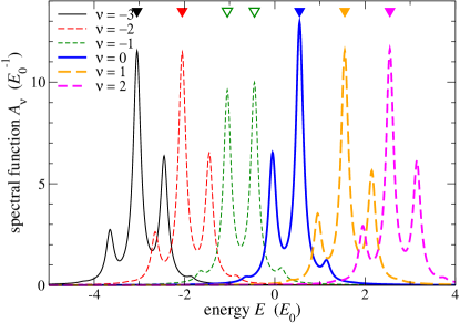
Figure 3: (Color online) Spectral function $A_{\nu}(E)$ for several states $|\nu\rangle$ with single-particle energies close to the Weyl node. The parameters are $eV=2E_{0}$, $e^{2}/C=0.6\,E_{0}$, and $eV_{g}=0.25\,E_{0}$, chosen so that there are no accidental degeneracies. The exchange fields in the barriers are parallel. The level spacing $E_{0}=\pi\hbar v_{F}/W$ is used as the energy unit. The energies of the strongest peaks are marked by triangles.

Figure 3 shows the spectral functions $A_{\nu}(E)$ for various $\nu$. The spectral functions for $\nu=-3,-2,1,2$, which correspond to large single-particle energies $|E_{\nu}|$, have similar shapes and mainly differ in shifts in energy. Their three-peak structure shows that three charge states of the dot dominate. Their shape is similar since the charge fluctuations mostly take place in other states, namely in $\nu=-1,0$. The spectral functions for $\nu=-1,0$ have only two dominant peaks because the charge in the other states assumes mainly two distinct values; the fluctuating occupation of the state $|\nu\rangle$ itself does not matter, see Eq. (43). Also note the phase change of the pattern for increasing $\nu$: The spectral functions $A_{\nu}(E)$ for large $\nu$ have an additional energy shift of $e^{2}/C$ compared to those for small $\nu$ since for large $\nu$ the total occupation of the other states is larger by one than for small $\nu$.

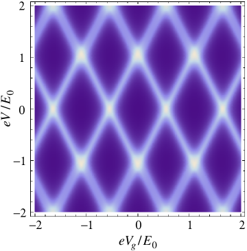
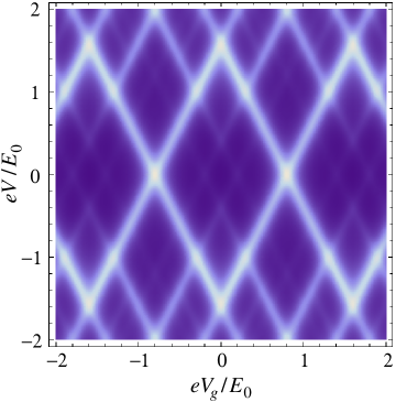
(a) (b) (c)

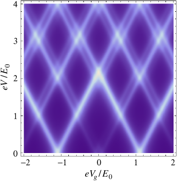
Figure 4: (Color online) Density plots of the differential conductance $dI/dV$ through a QSH quantum dot with parallel exchange fields as a function of gate voltage $V_{g}$ and bias voltage $V$. The dimensionless strength of the magnetic barriers is $\eta=1$ ($\gamma=0.086689\,E_{0}$). The interaction strength is (a) $e^{2}/C=0.1\,E_{0}$, (b) $e^{2}/C=0.6\,E_{0}$ (same as in Fig. 3), and (c) $e^{2}/C=1.2\,E_{0}$ (note the shifted vertical axis).

Figure 4 shows the differential conductance for various interaction strengths and otherwise the same parameters as in Fig. 2(a). With increasing interaction strength the Pauli-blockade diamonds morph into Coulomb-blockade diamonds and become larger, in agreement with the gate-voltage period $E_{0}+e^{2}/C$. Also, the sequential-tunneling peaks defining the Coulomb-blockade threshold gain more weight; recall that in the non-interacting case $dI/dV$ was periodic in the bias voltage $V$.

The differential-conductance plot in Fig. 4(b) corresponds to the spectral functions $A_{\nu}(E)$ shown in Fig. 3. The plots are not easy to compare, since the spectral functions are calculated for fixed bias voltage $V$, but one can say that the splitting of the peak in $A_{\nu}(E)$ due to interactions is reflected by a splitting of the sequential-tunneling peaks in $dI/dV$. Importantly, weaker conductance peaks are visible inside the Coulomb-blockade diamonds. While a single dot charge dominates in this regime, other dot charges have non-zero probabilities, which are controlled by the tails of the Lorentzian peaks. These subdominant dot charges lead to satellite peaks in the differential conductance.

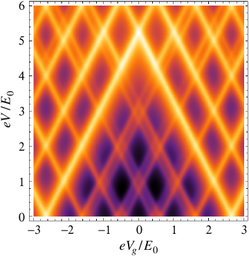
Figure 5: (Color online) Density plot of the differential conductance $dI/dV$ through a QSH quantum dot with parallel exchange fields as a function of gate voltage $V_{g}$ and bias voltage $V$ for strong electron-electron interaction $e^{2}/C=4.3\,E_{0}$. The dimensionless strength of the magnetic barriers is $\eta=1$. Other than in the previous figures the logarithm of $dI/dV$ is plotted, which enhances the contrast at small $dI/dV$. Also note the extended voltage scales.

(a)
(b)

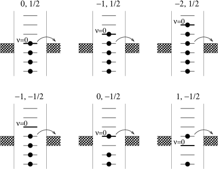
Figure 6: (a) Sketch of strong sequential-tunneling lines for the case of strong interaction, $e^{2}/C>E_{0}$. The lines sloping upward correspond to electrons tunneling out of the quantum dot. They are labeled by the number $\nu$ of the single-particle state involved and by the excess electron number $\Delta n_{\neg\nu}=\sum_{\mu\neq\nu}(m_{\mu}-1/2)$ of the other states. The bold lines denote the edges of the Coulomb-blockade diamonds. (b) Illustration of the tunneling processes responsible for the lines marked in panel (a) for $eV=0$ and $eV_{g}$ tuned so that the process is resonant.

Figure 5 shows $dI/dV$ for strong interaction, $e^{2}/C=4.3\,E_{0}$. Interestingly, the conductance peaks inside the Coulomb diamond show an approximate periodicity with the non-interacting periods $E_{0}$ in $eV_{g}$ and $2E_{0}$ in $eV$. Thus the non-interacting pattern re-emerges for strong interactions. Further inspection shows that there are two sets of lines, each with period $E_{0}$. The spectral-function peaks and tunneling processes corresponding to these features are illustrated in Fig. 6. The sequential tunneling lines are characterized by the state $|\nu\rangle$ involved in the tunneling and by the excess occupation number $\Delta n_{\neg\nu}$ of the other states. For strong interactions, at least one and typically only one peak resulting from $A_{\nu}(E)$ for fixed $\nu$ lies inside the Coulomb-blockade diamond. Figure 6 shows that there are two families of lines corresponding to $\Delta n_{\neg\nu}=1/2$ and $\Delta n_{\neg\nu}=-1/2$, respectively. (Additional families exist but correspond to initial states with larger excess charge and much smaller probability.)

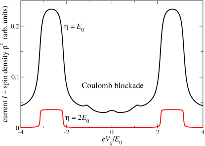
Figure 7: (Color online) Current as a function of gate voltage for bias voltage $eV=E_{0}$, interaction strength $e^{2}/C=4.3\,E_{0}$, and two strengths $\eta$ of the magnetic barriers, which have parallel exchange fields. The current is proportional to the uniform z-component of the spin density.

We now turn to the consequences of spin-momentum locking. From the continuity equation for the charge, $\partial_{t}\rho+\partial_{x}j=0$, one easily obtains the charge current in terms of the many-particle wave function $\Psi$,

$$j(x)=-ev_{F}\int dx_{1}dx_{2}\ldots\sum_{\sigma_{1}\sigma_{2}\ldots=\pm 1}\sum_{i}\delta(x-x_{i})$$ (51)

$${}\times\Psi^{\ast}_{\sigma_{1}\sigma_{2}\ldots}(x_{1},x_{2},\ldots)\,\sigma_{i}\,\Psi_{\sigma_{1}\sigma_{2}\ldots}(x_{1},x_{2},\ldots).\quad$$

This expression is clearly proportional to the z-component of the spin density $\rho^{z}$,

$$j(x)=-\frac{2ev_{F}}{\hbar}\,\rho^{z}(x).$$ (52)

In the stationary state, the current $j(x)=I$ is uniform so that the z-component of the spin density is also uniform and given by $\rho^{z}=-{\hbar I}/{2ev_{F}}$. Thus the quantum-dot structure permits to control the magnetization of the whole edge with a gate voltage applied locally to the dot. We do not address the dynamics in this paper, i.e., we do not study how the edge reacts to a non-adiabatic change of the gate voltage. Figure 7 shows the uniform current (spin-z density) as a function of the gate voltage for strong interaction, $e^{2}/C=4.3\,E_{0}$, corresponding to Fig. 5. For stronger magnetic barriers, the current and the spin density are reduced but the contrast between sequential-tunneling (“on”) and Coulomb-blockade (“off”) regimes is higher.

Equation (52) begs the question whether the z-component of the spin current is related to the charge density. Indeed, from the spin continuity equation $\partial_{t}\rho^{z}+\partial_{x}j^{z}=0$ one obtains the spin current

$$j^{z}(x) = \frac{\hbar v_{F}}{2}\int dx_{1}dx_{2}\ldots\sum_{\sigma_{1}\sigma_{2}\ldots=\pm 1}\sum_{i}\delta(x-x_{i})\,$$ (53)

$${}\times\Psi^{\ast}_{\sigma_{1}\sigma_{2}\ldots}(x_{1},x_{2},\ldots)\,\Psi_{\sigma_{1}\sigma_{2}\ldots}(x_{1},x_{2},\ldots)$$

$$= -\frac{\hbar v_{F}}{2e}\,\rho(x).$$

This result does not hold in the magnetic barriers, since spin is not conserved there. For the same reason, the spin-z current and thus the charge density are generally not continuous through the barriers. An exact result can be obtained at $eV_{g}=0$ for both parallel and antiparallel exchange fields: Here we have $\rho(x)=0$ and thus $j^{z}(x)=0$ within the dot for arbitrary bias voltage due to particle-hole symmetry.

The approximations involved in describing the coupling to the leads by a non-hermitian Hamiltonian and in truncating the equations of motion for the Green functions as shown in Appendix A may appear to be unsystematic. Insight into their meaning can be gained from an alternative derivation of the same final expression for the current. Since we calculate the stationary probabilities $P(\vec{m})$ in an effective tunneling picture with bare tunneling rate $R_{0}$ for each lead, it is natural to write down the current in the same picture. In the genealized sequential-tunneling approximation including level broadening, the current through lead $\alpha$ isBrF04 ; KOO04 ; TiE06

$$I^{\alpha}=-\alpha\,\frac{e}{\hbar}\sum_{\vec{m},\vec{m}^{\prime}}\bigg{(}\sum_{\nu}m_{\nu}^{\prime}-\sum_{\nu}m_{\nu}\bigg{)}\,R^{\alpha}_{\vec{m}\to\vec{m}^{\prime}}\,P(\vec{m}),$$ (54)

where $\alpha=L=1$ ($\alpha=R=-1$) for the left (right) lead. $R^{\alpha}_{\vec{m}\to\vec{m}^{\prime}}$ denotes the part of the rates in Eqs. (48) and (49) due to lead $\alpha$. For the symmetrized current we obtain, using an obvious notation,

$$I = \frac{I^{L}+I^{R}}{2}\;=\;-\frac{e}{2\hbar}\sum_{\vec{m}}\sum_{\nu}$$ (57)

$${}\times\left\{\begin{array}[]{cl}R_{\nu}^{L,\mathrm{in}}-R_{\nu}^{R,\mathrm{in}}&\mbox{for $m_{\nu}=0$}\\[4.30554pt] -R_{\nu}^{L,\mathrm{out}}+R_{\nu}^{R,\mathrm{out}}&\mbox{for $m_{\nu}=1$}\end{array}\right\}\,P(\vec{m}).\qquad$$

We reobtain Eq. (44) for the current if we assume that the scale of the sequential-tunneling rates is the coupling function $R_{0}=\Gamma^{L}=\Gamma^{R}$. This is plausible but was not a-priori obvious since our Hamiltonian is not of tunneling form. The approximations used in the first approach to find the mapping of the probabilites $P(\vec{m})$ to the current are thus equivalent to a sequential-tunneling approximation with additional level broadening. The first approach has the advantages of also providing the spectral functions $A_{\nu}(E)$ and of being suitable for approximations other than perturbation theory for weak coupling.

V Summary

We have considered a quantum dot in a QSH edge realized by two thin magnetic tunneling barriers with parallel or antiparallel exchange fields. For vanishing electron-electron interactions, the linear dispersion of edge states leads to an equidistant ladder of dot resonances and to a double periodicity of the differential conductance in both gate and bias voltage. The results can be analyzed within the framework of Meir-Wingreen theory for arbitrary coupling between dot and leads although the Hamiltonian is not of tunneling form.

In the interacting case, an equation-of-motion approach for the local retarded Green function yields a multiple-peak structure in the spectral function, where the peaks result from distinct charge states of the dot. Their probabilities are calculated within a rate-equation approach, which is valid for high magnetic tunneling barriers. The approach also becomes exact in the two limits of vanishing tunneling barriers and of weak interactions. We have calculated and analyzed the differential conductance from weak to strong Coulomb interaction on the dot. For increasing interaction strength, the Coulomb-blockade diamonds grow in size. The periodicity in the gate voltage is retained, while the periodicity in the bias voltage is destroyed. For stronger interactions, weak tunneling peaks appear inside the Coulomb-blockade diamonds. For very stong interactions compared to the spacing of the dot resonances, two copies of the non-interacting periodic pattern re-emerge inside the diamonds.

Spin-momentum locking leads to an obvious proportionality between the charge current and the z-component of the spin density or magnetization in the whole QSH edge. This should make it possible to control the magnetization by a locally applied gate voltage.

Appendix A Evaluation of the equation of motion

In the following solution of the equation of motion (37) we set $\hbar=1$. Equation (37) contains the commutator

$$[H_{\mathrm{int}},c_{\nu}]=\frac{e^{2}}{2C}\sum_{\mu\mu^{\prime}}\left[\left(n_{\mu}-\frac{1}{2}\right)\left(n_{\mu^{\prime}}-\frac{1}{2}\right),c_{\nu}\right]=-\frac{e^{2}}{C}\sum_{\mu\neq\nu}\left(n_{\mu}-\frac{1}{2}\right)\,c_{\nu}.$$ (58)

Noting that $n_{\mu}$ and $H_{\mathrm{int}}$ commute with $K_{\mathrm{dot}}$, it follows that

$$e^{iK_{\mathrm{dot}}t}\,[H_{\mathrm{int}},c_{\nu}]\,e^{-iK_{\mathrm{dot}}t} = -\frac{e^{2}}{C}\sum_{\mu\neq\nu}\left(n_{\mu}-\frac{1}{2}\right)\,e^{iK_{\mathrm{dot}}t}\,c_{\nu}\,e^{-iK_{\mathrm{dot}}t}$$ (59)

$$= -\frac{e^{2}}{C}\,e^{-iE_{\nu}t-\gamma t}\sum_{\mu\neq\nu}\left(n_{\mu}-\frac{1}{2}\right)\,e^{iH_{\mathrm{int}}t}c_{\nu}e^{-iH_{\mathrm{int}}t}$$

$$= -\frac{e^{2}}{C}\,e^{-iE_{\nu}t-\gamma t}\sum_{\mu\neq\nu}\left(n_{\mu}-\frac{1}{2}\right)\,\exp\Bigg{(}-i\,\frac{e^{2}}{C}\sum_{\mu^{\prime}\neq\nu}\left(n_{\mu^{\prime}}-\frac{1}{2}\right)t\Bigg{)}\,c_{\nu}.$$

Next, we have to evaluate the anticommutator $\big{\{}e^{iK_{\mathrm{dot}}t}\,[H_{\mathrm{int}},c_{\nu}]\,e^{-iK_{\mathrm{dot}}t},c_{\nu^{\prime}}^{\dagger}\big{\}}$. For the diagonal case $\nu=\nu^{\prime}$, we immediately get

$$\{e^{iK_{\mathrm{dot}}t}\,[H_{\mathrm{int}},c_{\nu}]\,e^{-iK_{\mathrm{dot}}t},c_{\nu}^{\dagger}\}=-\frac{e^{2}}{C}\,e^{-iE_{\nu}t-\gamma t}\sum_{\mu\neq\nu}\left(n_{\mu}-\frac{1}{2}\right)\,\exp\Bigg{(}-i\,\frac{e^{2}}{C}\sum_{\mu^{\prime}\neq\nu}\left(n_{\mu^{\prime}}-\frac{1}{2}\right)t\Bigg{)}$$ (60)

$$=-\frac{e^{2}}{C}\,e^{-iE_{\nu}t-\gamma t}\sum_{\mu\neq\nu}\left(n_{\mu}-\frac{1}{2}\right)\,\prod_{\mu^{\prime}\neq\nu}\left[\exp\left(i\,\frac{e^{2}}{2C}\,t\right)\,(1-n_{\mu^{\prime}})+\exp\left(-i\,\frac{e^{2}}{2C}\,t\right)\,n_{\mu^{\prime}}\right]$$

$$=-i\,e^{-iE_{\nu}t-\gamma t}\,\frac{\partial}{\partial t}\,\prod_{\mu\neq\nu}\left[\exp\left(i\,\frac{e^{2}}{2C}\,t\right)\,(1-n_{\mu})+\exp\left(-i\,\frac{e^{2}}{2C}\,t\right)\,n_{\mu}\right],\hskip 100.00015pt$$

while for $\nu\neq\nu^{\prime}$ we find

$$\{e^{iK_{\mathrm{dot}}t}\,[H_{\mathrm{int}},c_{\nu}]\,e^{-iK_{\mathrm{dot}}t},c_{\nu^{\prime}}^{\dagger}\}=\frac{e^{2}}{C}\,e^{-iE_{\nu}t-\gamma t}\,\Bigg{[}\sum_{\mu\neq\nu}\left(n_{\mu}-\frac{1}{2}\right)\,\exp\Bigg{(}-i\,\frac{e^{2}}{C}\sum_{\mu^{\prime}\neq\nu}\left(n_{\mu^{\prime}}-\frac{1}{2}\right)t\Bigg{)},c_{\nu^{\prime}}^{\dagger}c_{\nu}\Bigg{]}$$ (61)

$$=2\,e^{-iE_{\nu}t-\gamma t}\,\frac{\partial}{\partial t}\,\sin\left(\frac{e^{2}}{2C}\,t\right)\,\prod_{\mu\neq\nu,\nu^{\prime}}\left[\exp\left(i\,\frac{e^{2}}{2C}\,t\right)\,(1-n_{\mu})+\exp\left(-i\,\frac{e^{2}}{2C}\,t\right)\,n_{\mu}\right]\,c_{\nu^{\prime}}^{\dagger}c_{\nu}.\hskip 50.00008pt$$

The equation of motion for the diagonal components of the Green function thus reads

$$(E-E_{\nu}+i\,\gamma)\,G^{\mathrm{ret}}_{\nu\nu}(E)=1+\int_{0}^{\infty}dt\,e^{-iE_{\nu}t-\gamma t}\,\frac{\partial}{\partial t}\,\left\langle\prod_{\mu\neq\nu}\left[\exp\left(i\,\frac{e^{2}}{2C}\,t\right)\,(1-n_{\mu})+\exp\left(-i\,\frac{e^{2}}{2C}\,t\right)\,n_{\mu}\right]\right\rangle$$ (62)

$$=-\int_{0}^{\infty}dt\,i\,(E-E_{\nu}+i\gamma)\,e^{i(E-E_{\nu})t-\gamma t}\,\left\langle\prod_{\mu\neq\nu}\left[\exp\left(i\,\frac{e^{2}}{2C}\,t\right)\,(1-n_{\mu})+\exp\left(-i\,\frac{e^{2}}{2C}\,t\right)\,n_{\mu}\right]\right\rangle.\hskip 30.00005pt$$

Hence, the diagonal Green function is

$$G^{\mathrm{ret}}_{\nu\nu}(E) = -i\int_{0}^{\infty}dt\,e^{i(E-E_{\nu})t-\gamma t}\,\left\langle\prod_{\mu\neq\nu}\left[\exp\left(i\,\frac{e^{2}}{2C}\,t\right)\,(1-n_{\mu})+\exp\left(-i\,\frac{e^{2}}{2C}\,t\right)\,n_{\mu}\right]\right\rangle$$ (65)

$$= -i\int_{0}^{\infty}dt\,e^{i(E-E_{\nu})t-\gamma t}\sum_{\ldots,m_{0},m_{1},\ldots=0}^{1}\left\langle\prod_{\mu\neq\nu}\exp\left((-1)^{m_{\mu}}i\,\frac{e^{2}}{2C}\,t\right)\,\left\{\begin{array}[]{cl}1-n_{\mu}&\mbox{for $m_{\mu}=0$}\\ n_{\mu}&\mbox{for $m_{\mu}=1$}\end{array}\right\}\right\rangle$$

$$= \sum_{\ldots,m_{0},m_{1},\ldots=0}^{1}\left\langle\prod_{\mu\neq\nu}\left\{\begin{array}[]{cl}1-n_{\mu}&\mbox{for $m_{\mu}=0$}\\ n_{\mu}&\mbox{for $m_{\mu}=1$}\end{array}\right\}\right\rangle\,\frac{1}{E-E_{\nu}-\frac{e^{2}}{C}\sum_{\mu\neq\nu}\left(n_{\mu}-\frac{1}{2}\right)+i\gamma}.\hskip 50.00008pt$$ (68)

The sum is over all $m_{\mu}$ with $\mu\neq\nu$.

For the off-diagonal components, $\nu\neq\nu^{\prime}$, inserting Eq. (61) into the equation of motion (37) gives

$$(E-E_{\nu}+i\,\gamma)\,G^{\mathrm{ret}}_{\nu\nu^{\prime}}(E)=2i\int_{0}^{\infty}dt\,e^{-iE_{\nu}t-\gamma t}\,\frac{\partial}{\partial t}\,\sin\left(\frac{e^{2}}{2C}\,t\right)$$ (69)

$$\quad{}\times\left\langle\prod_{\mu\neq\nu,\nu^{\prime}}\left[\exp\left(i\,\frac{e^{2}}{2C}\,t\right)\,(1-n_{\mu})+\exp\left(-i\,\frac{e^{2}}{2C}\,t\right)\,n_{\mu}\right]\,c_{\nu^{\prime}}^{\dagger}c_{\nu}\right\rangle$$

$$=2\int_{0}^{\infty}dt\,(E-E_{\nu}+i\gamma)\,e^{i(E-E_{\nu})t-\gamma t}\,\sin\left(\frac{e^{2}}{2C}\,t\right)$$

$$\quad{}\times\left\langle\prod_{\mu\neq\nu,\nu^{\prime}}\left[\exp\left(i\,\frac{e^{2}}{2C}\,t\right)\,(1-n_{\mu})+\exp\left(-i\,\frac{e^{2}}{2C}\,t\right)\,n_{\mu}\right]\,c_{\nu^{\prime}}^{\dagger}c_{\nu}\right\rangle.$$

Performing the integral, we obtain the off-diagonal Green function

$$G^{\mathrm{ret}}_{\nu\nu^{\prime}}(E) = \sum_{\ldots,m_{0},m_{1},\ldots=0}^{1}\left\langle\prod_{\mu\neq\nu,\nu^{\prime}}\left\{\begin{array}[]{cl}1-n_{\mu}&\mbox{for $m_{\mu}=0$}\\ n_{\mu}&\mbox{for $m_{\mu}=1$}\end{array}\right\}\,c_{\nu^{\prime}}^{\dagger}c_{\nu}\right\rangle$$ (73)

$${}\times\left(\frac{1}{E-E_{\nu}-\frac{e^{2}}{C}\sum_{\mu\neq\nu}\left(n_{\mu}-\frac{1}{2}\right)+\frac{e^{2}}{2C}+i\gamma}-\frac{1}{E-E_{\nu}-\frac{e^{2}}{C}\sum_{\mu\neq\nu}\left(n_{\mu}-\frac{1}{2}\right)-\frac{e^{2}}{2C}+i\gamma}\right),$$

where the sum is now over all $m_{\mu}$ with $\mu\neq\nu,\nu^{\prime}$. The off-diagonal components of the Green function thus contain averages involving the off-diagonal operator $c_{\nu^{\prime}}^{\dagger}c_{\nu}$. In the stationary state such averages vanish: For the average in Eq. (73) to be non-zero, the stationary-state reduced density operator $\rho$ would have to be non-diagonal in the occupation-number basis. Specifically, superpositions of states different by a single electron being transferred from $|\nu\rangle$ to $|\nu^{\prime}\rangle$ would have to occur. From the decoupled dot Hamiltonian, such off-diagonal components of $\rho$ obtain a rotating phase factor with frequency $\omega=|E_{\nu^{\prime}}-E_{\nu}|/\hbar\neq 0$. For the stationary state, this time dependence would have to be canceled by the time dependence due to the coupling to the leads. That this cannot happen follows for example from the fact that the leads do not contain the energy scale $E_{0}=\pi\hbar v_{F}/W$.

References

- (1) M. Z. Hasan and C. L. Kane, Rev. Mod. Phys. 82, 3045 (2010).
- (2) S. Ryu, A. Schnyder, A. Furusaki, and A. Ludwig, New J. Phys. 12, 065010 (2010).
- (3) X.-L. Qi and S.-C. Zhang, arXiv:1008.2026, to be published in Rev. Mod. Phys.
- (4) A. P. Schnyder, S. Ryu, A. Furusaki, and A. W. W. Ludwig, Phys. Rev. B 78, 195125 (2008); AIP Conf. Proc. 1134, 10 (2009).
- (5) A. Yu. Kitaev, AIP Conf. Proc. 1134, 22 (2009).
- (6) M. R. Zirnbauer, J. Math. Phys. 37, 4986 (1996); A. Altland and M. R. Zirnbauer, Phys. Rev. B 55, 1142 (1997).
- (7) S. Murakami, N. Nagaosa, and S. C. Zhang, Science 301, 1348 (2003); Phys. Rev. Lett. 93, 156804 (2004).
- (8) J. Sinova, D. Culcer, Q. Niu, N. A. Sinitsyn, T. Jungwirth, and A. H. MacDonald, Phys. Rev. Lett. 92, 126603 (2004).
- (9) B. A. Bernevig, T. L. Hughes, and S. C. Zhang, Science 314, 1757 (2006).
- (10) M. König, S. Wiedmann, C. Brüne, A. Roth, H. Buhmann, L. W. Molenkamp, X.-L. Qi, and S.-C. Zhang, Science 318, 766 (2007).
- (11) M. König, H. Buhmann, L. W. Molenkamp, T. Hughes, C.-X. Liu, X.-L. Qi, and S.-C. Zhang, J. Phys. Soc. Jpn. 77, 031007 (2008).
- (12) G. Tkachov and E. M. Hankiewicz, Phys. Rev. B 83, 155412 (2011).
- (13) R. Landauer, IBM J. Res. Dev. 1, 233 (1957); Philos. Mag. 21, 863 (1970).
- (14) Y. Meir and N. S. Wingreen, Phys. Rev. Lett. 68, 2512 (1992).
- (15) A.-P. Jauho, N. S. Wingreen, and Y. Meir, Phys. Rev. B 50, 5528 (1994).
- (16) C. Wu, B. A. Bernevig, and S.-C. Zhang, Phys. Rev. Lett. 96, 106401 (2006).
- (17) C. Xu and J. E. Moore, Phys. Rev. B 73, 045322 (2006).
- (18) J. C. Budich, F. Dolcini, P. Recher, and B. Trauzettel, arXiv:1109.5188 (unpublished).
- (19) C. L. Kane and M. P. A. Fisher, Phys. Rev. B 46, R7268 (1992); 46, 15233 (1992).
- (20) A. Furusaki and N. Nagaosa, Phys. Rev. B 47, 3827 (1993).
- (21) C. Chamon and X. G. Wen, Phys. Rev. Lett. 70, 2605 (1993).
- (22) V. Meden, T. Enss, S. Andergassen, W. Metzner, and K. Schönhammer, Phys. Rev. B 71, 041302(R) (2005).
- (23) K. T. Law, C. Y. Seng, P. A. Lee, and T. K. Ng, Phys. Rev. B 81, 041305(R) (2010).
- (24) J. I. Väyrynen and T. Ojanen, Phys. Rev. Lett. 106, 076803 (2011).
- (25) Due to spin-momentum locking, the probability current density equals and is automatically continuous when the boundary condition (6) is satisfied.
- (26) J. A. Appelbaum, Phys. Rev. 154, 633 (1967).
- (27) K. R. Patton, arXiv:1007.1238 (unpublished).
- (28) The spurious self-interaction term appearing in the Hartree approximation is removed by the Fock term.
- (29) D. M.-T. Kuo and Y.-C. Chang, Phys. Rev. Lett. 99, 086803 (2007); Y.-C. Chang and D. M.-T. Kuo, Phys. Rev. B 77, 245412 (2008).
- (30) Y. Meir, N. S. Wingreen, and P. A. Lee, Phys. Rev. Lett. 66, 3048 (1991).
- (31) R. Zwanzig, J. Chem. Phys. 33, 1338 (1960).
- (32) S. Koller, M. Leijnse, M. R. Wegewijs, and M. Grifoni, Phys. Rev. B 82, 235307 (2010).
- (33) C. Timm, Phys. Rev. B 83, 115416 (2011).
- (34) H. Schoeller and G. Schön, Phys. Rev. B 50, 18436 (1994).
- (35) H. Bruus and K. Flensberg, Many-body Quantum Theory in Condensed Matter Physics (Oxford University Press, Oxford, 2004).
- (36) J. Koch, F. von Oppen, Y. Oreg, and E. Sela, Phys. Rev. B 70, 195107 (2004).
- (37) C. Timm and F. Elste, Phys. Rev. B 73, 235304 (2006).