Perron vector optimization applied to search engines

Abstract

In the last years, Google’s PageRank optimization problems have been extensively studied. In that case, the ranking is given by the invariant measure of a stochastic matrix. In this paper, we consider the more general situation in which the ranking is determined by the Perron eigenvector of a nonnegative, but not necessarily stochastic, matrix, in order to cover Kleinberg’s HITS algorithm. We also give some results for Tomlin’s HOTS algorithm. The problem consists then in finding an optimal outlink strategy subject to design constraints and for a given search engine.

We study the relaxed versions of these problems, which means that we should accept weighted hyperlinks. We provide an efficient algorithm for the computation of the matrix of partial derivatives of the criterion, that uses the low rank property of this matrix. We give a scalable algorithm that couples gradient and power iterations and gives a local minimum of the Perron vector optimization problem. We prove convergence by considering it as an approximate gradient method.

We then show that optimal linkage stategies of HITS and HOTS optimization problems verify a threshold property. We report numerical results on fragments of the real web graph for these search engine optimization problems.

1 Introduction

Motivation

Internet search engines use a variety of algorithms to sort web pages based on their text content or on the hyperlink structure of the web. In this paper, we focus on algorithms that use the latter hyperlink structure, called link-based algorithms. The basic notion for all these algorithms is the web graph, which is a digraph with a node for each web page and an arc between pages $i$ and $j$ if there is a hyperlink from page $i$ to page $j$. Famous link-based algorithms are PageRank [7], HITS [26], SALSA [27] and HOTS [49]. See also [28, 29] for surveys on these algorithms. The main problem of this paper is the optimization of the ranking of a given web site. It consists in finding an optimal outlink strategy maximizing a given ranking subject to design constraints.

One of the main ranking methods relies on the PageRank introduced by Brin and Page [7]. It is defined as the invariant measure of a walk made by a random surfer on the web graph. When reading a given page, the surfer either selects a link from the current page (with a uniform probability), and moves to the page pointed by that link, or interrupts his current search, and then moves to an arbitrary page, which is selected according to given “zapping” probabilities. The rank of a page is defined as its frequency of visit by the random surfer. It is interpreted as the “popularity” of the page. The PageRank optimization problem has been studied in several works: [1, 35, 14, 22, 13, 17]. The last two papers showed that PageRank optimization problems have a Markov decision process structure and both papers provided efficient algorithm that converge to a global optimum. Csáji, Jungers and Blondel in [13] showed that optimizing the PageRank score of a single web page is a polynomial problem. Fercoq, Akian, Bouhtou and Gaubert in [17] gave an alternative Markov decision process model and an efficient algorithm for the PageRank optimization problem with linear utility functions and more general design constraints, showing in particular that any linear function of the PageRank vector can be optimized in polynomial time.

In this paper, we consider the more general situation in which the ranking is determined by the Perron eigenvector of a nonnegative, but not necessarily stochastic, matrix. The Perron-Frobenius theorem (see [6] for instance) states that any nonnegative matrix $A$ has a nonnegative principal eigenvalue called the Perron root and nonnegative principal eigenvectors. If, in addition, $A$ is irreducible, then the Perron root is simple and the (unique up to a multiplicative constant) nonnegative eigenvector, called the Perron vector, has only positive entries. This property makes it a good candidate to sort web pages. The ranking algorithms considered differ in the way of constructing from the web graph a nonnegative irreducible matrix from which we determine the Perron vector. Then, the bigger is the Perron vector’s coordinate corresponding to a web page, the higher this web page is in the ranking. In [24], such a ranking is proposed for football teams. The paper [46] uses the Perron vector to rank teachers from pairwise comparisons. See also [50] for a survey on the subject. When it comes to web page ranking, the PageRank is the Perron eigenvector of the transition matrix described above but the HITS and SALSA algorithms also rank pages according to a Perron vector.

The HITS algorithm [26] is not purely a link-based algorithm. It is composed of two steps and the output depends on the query of the user. Given a query, we first select a seed of pages that are relevant to the query according to their text content. This seed is then extended with pages linking to them, pages to which they link and all the hyperlinks between the pages selected. We thus obtain a subgraph of the web graph focused on the query. Then, the second step assigns each page two scores: a hub score $v$ and an authority score $u$ such that good hubs should point to good authorities and good authorities should be pointed to by good hubs. Introducing the adjacency matrix $A$ of the focused graph, this can be written as $v=\rho Au$ and $u=\rho A^{T}v$ with $\rho\in\mathbb{R}_{+}$, which means that the vector of hub scores is the Perron eigenvector of the matrices $A^{T}A$ and that the vector of authority scores is the Perron eigenvector of $AA^{T}$. The construction of HITS’ focused subgraph is a combination of text content relevancy with the query and of hyperlink considerations. Maximizing the probability of appearance of a web page on this subgraph is thus a composite problem out of the range of this paper. We shall however study the optimization of HITS authority, for a given focused subgraph.

The SALSA algorithm [27] shares the same first step as HITS. The second step consists in the computation of the invariant measure of a stochastic matrix which consists in a normalization of the rows of $A^{T}A$. In fact, with natural assumptions, this measure is proportionnal to the indegree of the web page. The authors show that the interest of the ranking algorithm lies in the combination of the two steps and not in one or the other alone. Thus from a hyperlink point of view, optimizing the rank in SALSA simply consists in maximizing the number of hyperlinks pointing to the target page. We shall not study SALSA optimization any further.

We also studied the optimization of Tomlin’s HOTS scores [49]. In this case, the ranking is the vector of dual variables of an optimal flow problem. The flow represents an optimal distribution of web surfers on the web graph in the sense of entropy minimization. The dual variable, one by page, is interpreted as the “temperature” of the page, the hotter a page the better. Tomlin showed that this vector is solution of a nonlinear fix point equation: it may be seen as a nonlinear eigenvector. Indeed, we show that most of the arguments available in the case of Perron vector optimization can be adapted to HOTS optimization. We think that this supports Tomlin’s remark that ”malicious manipulation of the dual values of a large scale nonlinear network optimization model […] would be an interesting topic“.

Contribution

In this paper, we study the problem of optimizing the Perron eigenvector of a controlled matrix and apply it to PageRank, HITS and HOTS optimization. Our first main result is the development of a scalable algorithm for the local optimization of a scalar function of the Perron eigenvector over a set of nonnegative irreducible matrices. Indeed, the global Perron vector optimization over a convex set of nonnegative matrices is NP-hard, so we focus on the searching of local optima. We give in Theorem 1 a power-type algorithm for the computation of the matrix of the partial derivatives of the objective, based on the fact that it is a rank 1 matrix. This theorem shows that computing the partial derivatives of the objective has the same computational cost as computing the Perron vector by the power method, which is the usual method when dealing with the large and sparse matrices built from the web graph. Then we give an optimization algorithm that couples power and gradient iterations (Algorithms 2 and 3). Each step of the optimization algorithm involves a suitable number of power iterations and a descent step. By considering this algorithm to be an approximate projected gradient algorithm [41, 43], we prove that the algorithm converges to a stationary point (Theorem 2). Compared with the case when the number of power iterations is not adapted dynamically, we got a speedup between 3 and 20 in our numerical experiments (Section 7) together with a more precise convergence result.

Our second main result is the application of Perron vector optimization to the optimization of scalar functions of HITS authority or HOTS scores. We derive optimization algorithms and, thanks to the low rank of the matrix of partial derivatives, we show that the optimal linkage strategies of both problems satisfy a threshold property (Propositions 9 and 12). This property was already proved for PageRank optimization in [14, 17]. As in [22, 13, 17] we partition the set of potential links $(i,j)$ into three subsets, consisting respectively of the set of obligatory links, the set of prohibited links and the set of facultative links. When choosing a subset of the facultative links, we get a graph from which we get any of the three ranking vectors. We are then looking for the subset of facultative links that maximizes a given utility function. We also study the associated relaxed problems, where we accept weighted adjacency matrices. This assumes that the webmaster can influence the importance of the hyperlinks of the pages she controls, for instance by choosing the size of the font, the color or the position of the link within the page. In fact, we shall solve the relaxed problems and then give conditions or heuristics to get an admissible strategy for the discrete problems.

Related works

As explained in the first part of the introduction, this paper extends the study of PageRank optimization developped in [1, 35, 14, 22, 13, 17] to HITS authority [26] and HOTS [49] optimization.

We based our study of Perron eigenvector optimization on two other domains: eigenvalue optimization and eigenvector sensitivity. There is a vast literature on eigenvalue and eigenvector sensitivity with many domains of application (see the survey [20] for instance). These works cope with perturbations of a given system. They consider general square matrices and any eigenvalue or eigenvector. They give the directional derivatives of the eigenvalue and eigenvector of a matrix with respect to a given perturbation of this matrix [36, 34]. Perron eigenvalue and eigenvector sensitivity was developped in [15, 16].

This led to the development of eigenvalue optimization. In [12, 39, 48] the authors show that the minimization of a convex function of the eigenvalues of symmetric matrices subject to linear constraints is a convex problem and can be solved with semi-definite programming. Eigenvalue optimization of nonsymmetric matrices is a more difficult problem. In general, the eigenvalue is a nonconvex nonlipschitz function of the entries of the matrix. The last section of [30] proposes a method to reduce the nonsymmetric case to the symmetric case by adding (many) additional variables. Another approach is developped in [40]: the author derives descent directions and optimality conditions from the perturbation theory and uses so-called dual matrices.

In the context of population dynamics, the problem of the maximization of the growth rate of a population can be modeled by the maximization of the Perron value of a given family of matrices. This technique is used in [31] to identify the parameters of a population dynamic model, in [2] for chemotherapy optimization purposes. An approach based on branching Markov decision processes is presented in [45]. Perron value optimization also appears in other contexts like in the minimization of the interferences in a network [9].

Apart from the stochastic case which can be solved by Markov decision techniques, like for PageRank, the search for a matrix with optimal eigenvectors does not seem to have been much considered in the literature. Indeed, the problem is not well defined since when an eigenvalue is not simple, the associated eigenspace may have dimension greater than 1.

Organization

The paper is organized as follows. In Section 2, we introduce Perron eigenvector and eigenvalue optimization problems and show that these problems are NP-hard problems on convex sets of matrices. We also point out some problems solvable in polynomial time. In Section 3, we give in Theorem 1 a method for the efficient computation of the derivative of objective function. Then in Section 4, we give the coupled power and gradient iterations and its convergence proof. In Sections 5 and 6, we show how HITS authority optimization problems and HOTS optimization problems reduce to Perron vector optimization. Finally, we report numerical results on a fragment of the real web graph in Section 7.

2 Perron vector and Perron value optimization problems

Let $M\in\mathbb{R}^{n\times n}$ be a (elementwise) nonnegative matrix. We say that $M$ is irreducible if it is not similar to a block upper triangular matrix with two blocks via a permutation. Equivalently, define the directed graph with $n$ nodes and an edge between node $i$ and $j$ if and only if $M_{i,j}>0$: $M$ is irreducible if and only if this graph is strongly connected.

We denote by $\rho(M)$ the principal eigenvalue of the irreducible nonnegative matrix $M$, called the Perron root. By Perron-Frobenius theorem (see [6] for instance), we know that $\rho(M)>0$ and that this eigenvalue is simple. Given a normalization $N$, we denote by $u(M)$ the corresponding normalized eigenvector, called the Perron vector. The normalization is necessary since the Perron vector is only defined up to positive multiplicative constant. The normalization function $N$ should be homogeneous and we require $u(M)$ to verify $N(u(M))=1$. The Perron-Frobenius theorem asserts that $u(M)>0$ elementwise. The Perron eigenvalue optimization problem on the set $\mathcal{M}$ can be written as:

$$\min_{M\in\mathcal{M}}f(\rho(M))$$ (1)

The Perron vector optimization problem can be written as:

$$\min_{M\in\mathcal{M}}f(u(M))$$ (2)

We assume that $f$ is a real valued continuously differentiable function; $\mathcal{M}$ is a set of irreducible nonnegative matrices such that $\mathcal{M}=h(\mathcal{C})$ with $h$ continuously differentiable and $\mathcal{C}$ a closed convex set. These hypotheses allow us to use algorithms such as projected gradient for the searching of stationary points.

We next observe that the minimization of the Perron root and the optimization of a scalar function of the Perron vector are NP-hard problems and that only exceptional special cases appear to be polynomial time solvable by current methods. Consequently, we shall focus on the local resolution of these problems, with an emphasis on large sparse problems like the ones encountered for web applications. We consider the two following problems:

PERRONROOT_MIN: given a rational linear function $A:\mathbb{R}^{n\times n}\to\mathbb{R}^{m}$ and a vector $b$ in $\mathbb{Q}^{m}$, find a matrix $M$ that minimizes $\rho(M)$ on the polyhedral set $\{M\in\mathbb{R}^{n\times n}\;|\;A(M)\leq b\;,\;M\geq 0\}$.

PERRONVECTOR_OPT: given a rational linear function $A:\mathbb{R}^{n\times n}\to\mathbb{R}^{m}$, a vector $b$ in $\mathbb{Q}^{m}$, a rational function $f:\mathbb{R}^{n}\to\mathbb{R}$ and a rational normalization function $N$, find a matrix $M$ that minimizes $f(u(M))$ on the polyhedral set $\{M\in\mathbb{R}^{n\times n}\;|\;A(M)\leq b\;,\;M\geq 0\}$, where $u(M)$ verifies $N(u(M))=1$.

In general, determining whether all matrices in an interval family are stable is a NP-hard problem [10]. The corresponding problem for nonnegative matrices is to determine whether the maximal Perron root is smaller than a given number. Indeed, as the Perron root is a monotone function of the entries of the matrix (see Proposition 4 below), this problem is trivial on interval matrix families. However, we shall prove NP-hardness of PERRONROOT_MIN and PERRONVECTOR_OPT by reduction of linear multiplicative programming problem to each of these problems. The linear multiplicative problem is:

LMP: given a $n\times m$ rational matrix $A$ and a vector $b$ in $\mathbb{Q}^{m}$, find a vector $x\in\mathbb{R}^{n}$ that minimizes $x_{1}x_{2}$ on the polyhedral set $\{x\in\mathbb{R}^{n}\;|\;Ax\leq b\;,\;x_{1},x_{2}\geq 0\}$.

A theorem of Matsui [32] states that LMP is NP-hard. We shall need a slightly stronger result about a weak version of LMP:

Weak-LMP: given $\epsilon>0$, a $n\times m$ rational matrix $A$ and a vector $b$ in $\mathbb{Q}^{m}$, find a vector $x\in Q$ such that $x_{1}x_{2}\leq y_{1}y_{2}+\epsilon$ for all $y\in Q$, where $Q=\{x\in\mathbb{R}^{n}\;|\;Ax\leq b\;,\;x_{1},x_{2}\geq 0\}$.

Lemma 1.

Weak-LMP is a NP-hard problem.

Proof.

A small modification of the proof of Matsui [32] gives the result. If we replace $g(x_{0},y_{0})\leq 0$ by $g(x_{0},y_{0})\leq-2$ in Corollary 2.3 we remark that the rest of the proof still holds since $n^{4}p^{4n}+p^{2}-4p^{4n+1}\leq-2$ for all $n\geq 1$ and $p=n^{n^{4}}$. Then, with the notations of [32], we have proved that the optimal value of $P1(M)$ is less than or equal to $4p^{8n}-2$ if and only if $Mx=1$ has a $0-1$ valued solution and it is greater than or equal to $4p^{8n}$ if and only if $Mx=1$ does not have a $0-1$ valued solution. We just need to choose $\epsilon<2$ in problem $P1(M)$ to finish the proof of the lemma. ∎

Proposition 1.

PERRONROOT_MIN and PERRONVECTOR_OPT are NP-hard problems.

Proof.

We define the matrix $M$ by the matrix with lower diagonal equal to $x$ and $1$ on the top left corner:

$$M=\begin{pmatrix}0&0&\ldots&0&1\\ x_{1}&0&0&&0\\ 0&x_{2}&0&&\vdots\\ \vdots&&\ddots&\ddots&\vdots\\ 0&\ldots&0&x_{n}&0\end{pmatrix}\enspace.$$

We set the admissible set $X$ for the vector $x$ as $X=\{x\in\mathbb{R}^{m}|Ax\geq b,x\geq 0\}$ with a rational $p\times m$ matrix $A$ and a rational vector $b$ of length $p$.

For the eigenvector problem, we set the normalization $u_{1}=1$ and we take $f(u)=u_{n}$. We have $u_{n}=\rho$, so the complexity is the same for eigenvalue and eigenvector optimization is this context.

Now minimizing $\rho(M)$ is equivalent to minimizing $x_{1}x_{2}\ldots x_{n}$ because the n-th root is an nondecreasing function on $\mathbb{R}_{+}$. We thus just need to reduce in polynomial time the $\epsilon$-solvability of weak-LMP to the minimization of $x_{1}x_{2}\ldots x_{n}$ on $X$.

As $x\mapsto\log(x_{1}x_{2}\ldots x_{n})$ is a concave function, either the problem is unbounded or there exists an optimal solution that is an extreme point of the polyhedral admissible set (Theorem 3.4.7 in [8]). Hence, using Lemma 6.2.5 in [19] we see that we can define a bounded problem equivalent to the unbounded problem and with coefficients that have a polynomial encoding length: in the following, we assume that the admissible set is bounded.

Given a rational number $\epsilon>0$, a rational $p\times m$ matrix $A^{\prime}$ and a rational vector $b^{\prime}$ of length $p$, let $X^{\prime}:=\{x\in\mathbb{R}^{m}|A^{\prime}x\geq b^{\prime},x_{1}\geq 0,x_{2}\geq 0\}$ be a bounded polyhedron. Denoting $v_{2}:=\min_{x\in X^{\prime}}x_{1}x_{2}$, we are looking for $x^{\prime}\in X^{\prime}$ such that $\lvert y_{1}y_{2}-v_{2}\rvert\leq\epsilon$.

Compute $\underline{C}:=\min_{i\in[n]}\min_{x\in X^{\prime}}x_{i}$ and $\bar{C}:=\max_{i\in[n]}\max_{x\in X^{\prime}}x_{i}$ (linear programs). We first set $m_{0}=\bar{C}-\underline{C}+1$ so that $m_{0}>0$ and $m_{0}>-\underline{C}$ and $t^{m_{0}}\in\mathbb{R}^{n}$ defined by $t^{m_{0}}_{i}=0$ if $i\in\{1,2\}$ and $t^{m_{0}}_{i}=m$ if $i\geq 3$. Let

$$X_{0}:=\{x\in\mathbb{R}^{m}|A^{\prime}x\geq b^{\prime}-A^{\prime}t^{m_{0}},x\geq 0\}\enspace.$$

We have $v_{2}=\min_{x\in X^{\prime}}x_{1}x_{2}=\min_{x\in X_{0}}x_{1}x_{2}$. Let $v_{0}:=\min_{x\in X}x_{1}x_{2}\ldots x_{n}$. For all $x\in X_{0}$, we have

$$x_{1}x_{2}(m_{0}+\underline{C})^{n-2}\leq x_{1}x_{2}\ldots x_{n}\leq x_{1}x_{2}(m_{0}+\bar{C})^{n-2}\enspace,$$

so that $v_{2}(m_{0}+\underline{C})^{n-2}\leq v_{0}\leq v_{2}(m_{0}+\bar{C})^{n-2}$.

We now set

$$m:=\max\{-\underline{C}+2^{n-3}\frac{\bar{C}}{\epsilon}\frac{v_{0}}{(m_{0}+\underline{C})^{n-2}},\bar{C}-2\underline{C},1\}$$

and we define $t^{m}$ and $X$ in the same way as $t^{m_{0}}$ and $X_{0}$. Remark that $m$ an encoding length polynomial in the length of the entries. Let $v_{n}:=\min_{x\in X}x_{1}x_{2}\ldots x_{n}$. For all $x\in X$, we have $v_{2}(m+\underline{C})^{n-2}\leq v_{n}\leq v_{2}(m+\bar{C})^{n-2}$ and $x^{\prime}=x-t^{m}$ is a point of $X^{\prime}$ with $x^{\prime}_{1}x^{\prime}_{2}=x_{1}x_{2}$.

As $v_{2}(m_{0}+\underline{C})^{n-2}\leq v_{0}$, $m\geq-\underline{C}+2^{n-3}\frac{\bar{C}}{\epsilon}v_{2}$. As $m\geq\bar{C}-2\underline{C}$, $\frac{m+\underline{C}}{m+\bar{C}}\geq\frac{1}{2}$, so that $\frac{(m+\underline{C})^{n-2}}{(m+\bar{C})^{n-3}}\geq\frac{1}{2^{n-3}}(m+\underline{C})$ and $\frac{(m+\underline{C})^{n-2}}{(m+\bar{C})^{n-3}}\geq\frac{\bar{C}}{\epsilon}v_{2}$.

Denote $M:=(m+\underline{C})^{n-2}$ and $\Delta:=(m+\bar{C})^{n-2}-(m+\underline{C})^{n-2}$: $Mv_{2}\leq v_{n}\leq(M+\Delta)v_{2}$ We have $\Delta:=\sum_{k=0}^{n-3}\binom{n-2}{k}m^{k}\bar{C}^{n-2-k}-\sum_{k=0}^{n-3}\binom{n-2}{k}m^{k}\underline{C}^{n-2-k}\leq\bar{C}(m+\bar{C})^{n-3}$. Hence, $M\geq\frac{\Delta}{\epsilon}v_{2}$. As $\Delta\geq 0$, $M+\Delta\geq\frac{\Delta}{\epsilon}v_{2}$. We obtain

$$\epsilon\geq\frac{\Delta Mv_{2}}{M(M+\Delta)}=(\frac{1}{M}-\frac{1}{M+\Delta})Mv_{2}\geq v_{2}-\frac{v_{n}}{M+\Delta}\enspace.$$

Finally

$$\frac{v_{n}}{(m_{0}+\bar{C})^{n-2}}\leq v_{2}\leq\frac{v_{n}}{(m_{0}+\bar{C})^{n-2}}+\epsilon\enspace.$$

which proves that weak-LMP reduces to the minimization of $x_{1}x_{2}\ldots x_{n}$ on $X$. ∎

The general Perron eigenvalue optimization problem is NP-hard but we however point out some cases for which it is tractable. The following proposition is well known:

Proposition 2 ([25]).

The eigenvalue $\rho(M)$ is a log-convex function of the log of the entries of the nonnegative matrix $M$.

This means that $\log\circ\rho\circ\exp$ is a convex function, where $\exp$ is the componentwise exponential, namely if $0\leq\alpha\leq 1$ and $A$ and $B$ are two nonnegative $n\times n$ matrices then for $C_{i,j}=A_{i,j}^{\alpha}B_{i,j}^{1-\alpha}$, $\rho(C)\leq\rho(A)^{\alpha}\rho(B)^{1-\alpha}$.

Corollary 1.

The optimization problem

$$\min_{M\in\exp(\mathcal{C})}\rho(M)$$

with $\mathcal{C}$ convex is equivalent to the convex problem

$$\min_{L\in C}\log\circ\rho\circ\exp(L)$$

The difference between this proposition and the previous one is that here $\mathcal{M}=h(C)=\exp(C)$ whereas previously we had $h$ affine. This makes a big difference since an $\epsilon$-solution of a convex program can be found in polynomial time [11].

Remark 1.

The largest singular value (which is a norm) is a convex function of the entries of the matrix. For a symmetric matrix, the singular values are the absolute values of the eigenvalues. Thus minimizing the largest eigenvalue on a convex set of nonnegative symmetric matrices is a convex problem.

In order to solve the signal to interference ratio balancing problem, Boche and Schuber [9] give an algorithm for the global minimization of the Perron root when the rows of the controlled matrix are independently controlled, ie when the admissible set is of the form $\mathcal{Z}_{1}\times\ldots\times\mathcal{Z}_{n}$ and $z_{k}\in\mathcal{Z}_{k}$ is the $k^{th}$ row of the matrix.

Proposition 3 ([9]).

Let $\mathcal{Z}=\mathcal{Z}_{1}\times\ldots\times\mathcal{Z}_{n}$ and $\Gamma$ be a fixed positive diagonal matrix. If the $k^{th}$ row of the matrix $V(z)$ only depends on $z_{k}\in\mathcal{Z}_{k}$, $V(z)$ is irreducible for all $z\in\mathcal{Z}$ and if $V(z)$ is continuous on $\mathcal{Z}$ ($\mathcal{Z}$ can be discrete), then there exists a monotone algorithm that minimizes $\rho(\Gamma V(z))$ over $\mathcal{Z}$, in the sense that $\rho(\Gamma V(z_{n+1}))\leq\rho(\Gamma V(z_{n}))$ for all $n\geq 0$ and $\lim_{n}\rho(\Gamma V(z_{n}))=\min_{z\in\mathcal{Z}}\rho(\Gamma V(z))$.

Let $X$ be the admissible set of a Perron eigenvalue optimization problem. Denote $\pi_{i}$ the projection on the $i^{th}$ coordinate. Then the minimization of the Perron value over $\tilde{X}:=\pi_{1}(X)\times\ldots\times\pi_{n}(X)$ is a relaxation of the original problem which is solvable with the algorithm of Proposition 3 as soon as all matrices in $\tilde{X}$ are irreducible. We thus get a lower bound for the optimization of the Perron eigenvalue problem in a general setting. This is complementary with the local optimization approach developped in this article, which would yield an upper bound on the optimal value of this problem.

Remark 2.

As developped in [17], general PageRank optimization problems can be formulated as follows. Let $M$ be the transition matrix of PageRank and $\rho$ the associated occupation measure. When $M$ is irreducible, they are linked by the relation $M_{ij}=\frac{\rho_{ij}}{\sum_{k}\rho_{ik}}=h_{ij}(\rho)$, which yields our function $h$. We also have $u(h(\rho))_{i}=\sum_{k}\rho_{ik}$ and $\rho_{ij}=u(M)_{i}M_{ij}$.

If the set $\mathcal{C}$, which defines the design constraints of the webmaster, is a convex set of occupation measures, if $h$ is as defined above and if $f$ is a convex function, then

$$\min_{\rho\in\mathcal{C}}f(u(h(\rho)))$$

is a convex problem. Thus $\epsilon$-solutions of PageRank optimization problems can be found in polynomial-time. Details of this development and exact resolution for a linear $f$ can be found in [17].

3 A power-type algorithm for the evaluation of the derivative of a function of the principal eigenvector

We now turn to the main topic of this paper. We give in Theorem 1 a power-type algorithm for the evaluation of the partial derivatives of the principal eigenvector of a matrix with a simple principal eigenvalue.

We consider a matrix $M$ with a simple eigenvalue $\lambda$ and associated left and right eigenvectors $u$ and $v$. We shall normalize $v$ by the assumption $\sum_{i\in[n]}v_{i}u_{i}=1$. The derivatives of the eigenvalue of a matrix are well known and easy to compute:

Proposition 4 ([23] Section II.2.2).

Denoting $v$ and $u$ the left and right eigenvectors of a matrix $M$ associated to a simple eigenvalue $\lambda$, normalized such that $\sum_{i\in[n]}v_{i}u_{i}=1$, the derivative of $\lambda$ can be written as:

$$\frac{\partial\lambda}{\partial M_{ij}}=v_{i}u_{j}$$

In this section, we give a scalable algorithm to compute the partial derivatives of the function $f\circ u$, that to an irreducible nonnegative matrix $M$ associates the utility of its Perron vector. In other words we compute $g_{ij}=\sum_{k}\frac{\partial f}{\partial u_{k}}\frac{\partial u_{k}}{\partial M_{ij}}$. This algorithm is a sparse iterative scheme and it is the core of the optimization algorithms that we will then use for the large problems encountered in the optimization of web ranking.

We first recall some results on the derivatives of eigenprojectors (see [23] for more background). Throughout the end of the paper, we shall consider column vectors and row vectors will be written as the transpose of a column vector. Let $P$ be the eigenprojector of $M$ for the eigenvalue $\lambda$. One can easily check that as $\lambda$ is a simple eigenvalue, the spectral projector is $P=uv^{T}$ as soon as $v^{T}u=1$. We have the relation

$$\frac{\partial P}{\partial M_{ij}}=-SE_{ij}P-PE_{ij}S$$

where $E_{ij}$ is the $n\times n$ matrix with all entries zero except the $ij^{th}$ and $S=(M-\lambda I)^{\#}$ is the Drazin pseudo-inverse of $M-\lambda I$. This matrix $S$ also satisfies the equalities

$$S(M-\lambda I)=(M-\lambda I)S=I-P\quad\text{and}\quad SP=PS=0$$ (3)

When it comes to eigenvectors, we have to set a normalization for each of them. Let $N$ be the normalization function for the right eigenvector. We assume that it is differentiable at $u$ and that $N(\alpha u)=\alpha N(u)$ for all nonnegative scalars $\alpha$, which implies $\frac{\partial N}{\partial u}(u)\cdot u=N(u)$. We normalize $v$ by the natural normalization $\sum_{i}u_{i}v_{i}=1$.

Proposition 5 ([34]).

Let $M$ be a matrix with a simple eigenvalue $\lambda$ and associated eigenvector $u$ normalized by $N(u)=1$. We denote $S=(M-\lambda I)^{\#}$. Then the partial derivatives of the eigenvector are given by:

$$\frac{\partial u}{\partial M_{ij}}(M)=-Se_{i}u_{j}+(\nabla N(u)^{T}Se_{i}u_{j})u$$

where $e_{i}$ is the vector with $i^{th}$ entry equal to 1.

To simplify notations, we denote $\nabla f$ for $\nabla f(u)$ and $\nabla N$ for $\nabla N(u)$.

Corollary 2.

Let $M$ be a matrix with a simple eigenvalue $\lambda$ and associated eigenvector $u$ normalized by $N(u)=1$. The partial derivatives of the function $M\mapsto(f\circ u)(M)$ at $M$ are $g_{ij}=w_{i}u_{j}$, where the auxiliary vector $w$ is given by:

$$w^{T}=(-\nabla f^{T}+(\nabla f\cdot u)\nabla N^{T})S=(-\nabla f^{T}+(\nabla f\cdot u)p^{T})(M-\lambda I)^{\#}$$

Proof.

By Proposition 5, we deduce that

$$g_{ij}=\sum_{k}\frac{\partial f}{\partial u_{k}}(u(M))\frac{\partial u_{k}}{\partial M_{ij}}(M)=-\sum_{k}\frac{\partial f}{\partial u_{k}}S_{ki}u_{j}+\sum_{k}\frac{\partial f}{\partial u_{k}}u_{k}\sum_{l}\frac{\partial N}{\partial u_{l}}S_{li}u_{j}$$

which is the developed form the result. ∎

This simple corollary already improves the computation speed. Using Proposition 5 directly, one needs to compute $\frac{\partial P}{\partial M_{ij}}$ in every direction, which means the computation of a Drazin inverse and $2n^{2}$ matrix-vector products involving $M$ for the cmputation of $\left(\frac{\partial u}{\partial M_{ij}}\right)_{i,j\in[n]}$. With Corollary 2 we only need one matrix-vector product for the same result. The last difficulty is the computation of the Drazin inverse $S$. In fact, we do not need to compute the whole matrix but only to compute $S^{T}x$ for a given $x$. The next two propositions show how one can do it.

Proposition 6.

Let $M$ be a matrix with a simple eigenvalue $\lambda$ and associated eigenvector $u$ normalized by $N(u)=1$. The auxiliary vector $w$ of Corollary 2 is solution of the following invertible system

$$[w^{T},w_{n+1}]\begin{bmatrix}M-\lambda I&-u\\ \nabla N^{T}&0\end{bmatrix}=[-\nabla f^{T},0]\enspace.$$ (4)

where $w_{n+1}\in\mathbb{R}$.

Proof.

A nullspace argument similar to this of [36] shows that $\begin{bmatrix}M-\lambda I&-u\\ \nabla N^{T}&0\end{bmatrix}$ is invertible as soon as $\lambda$ is simple and $\nabla N^{T}u=1$. Then the solution $w$ of the system (4) verifies the equations $w^{T}(M-\lambda I)+w_{n+1}\nabla N^{T}=-\nabla f^{T}$ and $w^{T}u=0$. Multiplying the first equality by $u$ yields $w_{n+1}\nabla N^{T}u=-\nabla f^{T}u$ and multiplying it by $S$ yields $w^{T}(I-uv^{T})=-w_{n+1}\nabla N^{T}S-\nabla f^{T}S$. Putting all together, we get $w^{T}=(-\nabla f^{T}+(\nabla f^{T}u)\nabla N^{T})S$. ∎

The next proposition provides an iterative scheme to compute the evaluation of the auxiliary vector $w$ when we consider the principal eigenvalue.

Definition 1.

We say that a sequence $(x_{k})_{k\geq 0}$ converges to a point $x$ with a linear convergence rate $\alpha$ if $\limsup_{k\to\infty}\lVert x_{k}-x\rVert^{1/k}\leq\alpha$.

Proposition 7.

Let $M$ be a matrix with only one eigenvalue of maximal modulus $\rho=\lvert\lambda_{1}\rvert>\lvert\lambda_{2}\rvert$. With the same notations as in Corollary 2, we denote $\tilde{M}=\frac{1}{\rho}M$ and $z^{T}=\frac{1}{\rho}(-\nabla f^{T}+(\nabla f\cdot u)\nabla N^{T})$, and we fix a real row vector $w_{0}$. Then the fix point scheme defined by

$$\forall k\in\mathbb{N},\quad w^{T}_{k+1}=(-z^{T}+w^{T}_{k}\tilde{M})(I-P)$$

with $P=uv^{T}$, converges to $w^{T}=(-\nabla f^{T}+(\nabla f\cdot u)\nabla N^{T})(M-\rho I)^{\#}$ with a linear rate of convergence $\frac{\lvert\lambda_{2}\rvert}{\rho}$.

Proof.

We have $w^{T}_{k}=\sum_{l=0}^{k-1}-z^{T}(\tilde{M}(I-P))^{l}+w^{T}_{0}(\tilde{M}(I-P))^{k}$. By assumption, all the eigenvalues of $\tilde{M}$ different from $1$ have a modulus smaller than $1$. Thus, using the fact that $P$ is the eigenprojector associated to $1$, we get $\rho(\tilde{M}(I-P))=\frac{\lvert\lambda_{2}\rvert}{\rho}<1$. By [38], $(\lVert\tilde{M}(I-P)\rVert^{k})^{1/k}\to\rho(\tilde{M}(I-P))$, so the algorithm converges to a limit $w$ and for all $\epsilon>0$, $\lVert w_{k}-w\rVert=\text{\large O}((\frac{\lvert\lambda_{2}\rvert+\epsilon}{\rho})^{k})$. This implies a linear convergence rate equal to $\frac{\lvert\lambda_{2}\rvert}{\rho}$. The limit $w$ satisfies $w^{T}=(-z^{T}+w^{T}\tilde{M})(I-P)$, so $w^{T}P=0$ and as $\tilde{M}P=P$, $w^{T}\tilde{M}-w^{T}=z^{T}(I-P)$. We thus get the equality $w^{T}(\tilde{M}-I)=z^{T}$. Multiplying both sides by $(\tilde{M}-I)^{\#}$, we get:

$$w^{T}(\tilde{M}-I)(\tilde{M}-I)^{\#}=w^{T}-w^{T}P=w^{T}=z^{T}(\tilde{M}-I)^{\#}$$

The last equalities and the relation $(\beta^{-1}M)^{\#}=\beta M^{\#}$ show by Proposition 2 that $g=wu^{T}$ is the matrix of partial derivatives of the Perron vector multiplied by $\nabla f$. ∎

This iterative scheme uses only matrix-vector products and thus may be very efficient for a sparse matrix. In fact, it has the same linear convergence rate as the power method for the computation of the Perron eigenvalue and eigenvector. This means that the computation of the derivative of the eigenvector has a computational cost of the same order as the computation of the eigenvector itself. We next show that the eigenvector and its derivative can be computed in a single algorithm.

Theorem 1.

If $M$ is a matrix with only one simple eigenvalue of maximal modulus $\rho=\lvert\lambda_{1}\rvert>\lvert\lambda_{2}\rvert$, then the derivative $g$ of the function $f\circ u$ at $M$, such that $g_{ij}=\sum_{k}\frac{\partial f}{\partial u_{k}}\frac{\partial u_{k}}{\partial M_{ij}}$ is the limit of the sequence $(\tilde{w}_{l}u_{l}^{T})_{l\geq 0}$ given by the following iterative scheme:

$$u_{l+1} =\frac{Mu_{l}}{N(Mu_{l})}$$

$$v_{l+1}^{T} =\frac{v_{l}^{T}M}{v_{l}^{T}Mu_{l+1}}$$

$$\tilde{w}_{l+1}^{T} =\frac{1}{\rho_{l}}(\nabla f_{l}^{T}-(\nabla f_{l}\cdot u_{l})\nabla N_{l}^{T}+\tilde{w}_{l}^{T}M)(I-u_{l+1}v_{l+1}^{T})$$

where $\rho_{l}=N(Mu_{l})$, $\nabla f_{l}=\nabla f(u_{l})$ and $\nabla N_{l}=\nabla N(u_{l})$. Moreover, the sequences $(u_{l})$, $(v_{l})$ and $(\tilde{w}_{l})$ converge linearly with rate $\frac{\lvert\lambda_{2}\rvert}{\rho}$.

Of course, the first and second sequences are the power method to the right and to the left. The third sequence is a modification the scheme of Proposition 7 with currently known values only. We shall denote one iteration of the scheme of the theorem as

$$(u_{k+1},v_{k+1},\tilde{w}_{k+1})=\mathrm{POWERDERIVATIVE_{M}}(u_{k},v_{k},\tilde{w}_{k})\enspace.$$

Proof.

The equalities giving $u_{l+1}$ and $v_{l+1}$ are simply the usual power method, so by [42], they convergence linearly with rate $\frac{\lvert\lambda_{2}\rvert}{\rho}$ to $u$ and $v$, the right and left principal eigenvectors of $M$, such that $P=uv^{T}$ is the eigenprojector associated to $\rho(M)$. Let

$$z_{l}^{T}:=\frac{1}{\rho_{l}}(-\nabla f_{l}^{T}+(\nabla f_{l}\cdot u_{l})\nabla N_{l}^{T})\enspace:$$

$\lim z_{l}=z$ by continuity of $\nabla f$, $N$ and $\nabla N$ at $u$. We also have

$$\tilde{w}_{l}^{T}=(-z_{l}^{T}+\frac{1}{\rho_{l}}\tilde{w}_{l}^{T}M)(I-u_{l+1}v_{l+1}^{T})\enspace.$$

We first show that $\tilde{w}_{l}$ is bounded. As in the proof of Proposition 7, $\rho(\tilde{M}(I-P))=\frac{\lvert\lambda_{2}\rvert}{\rho}<1$. Thus, by Lemma 5.6.10 in [21], there exists a norm $\lVert\cdot\rVert_{M}$ and $\alpha<1$ such that $\tilde{M}(I-P)$ is $\alpha$-contractant. Let $S$ be the unit sphere: $\forall x\in S,\lVert\tilde{M}(I-P)x\rVert_{M}\leq\alpha\lVert x\rVert_{M}$. By continuity of the norm, $\forall\epsilon>0,\exists L,\forall l\geq L,\forall x\in S,\lVert\frac{1}{\rho_{l}}M(I-u_{l+1}v_{l+1}^{T})x\rVert_{M}\leq(\alpha+\epsilon)\lVert x\rVert_{M}$. As $\frac{1}{\rho_{l}}M(I-u_{l+1}v_{l+1}^{T})$ is linear, we have the result on the whole $\mathbb{R}^{n}$ space. Thus $\tilde{w}_{l}$ is bounded.

Let us denote $\tilde{M}=\frac{1}{\rho}M$ and

$$\tilde{z}_{l}^{T}:=z_{l}^{T}(I-u_{l+1}v_{l+1}^{T})+\frac{1}{\rho_{l}}\tilde{w}_{l}^{T}M(uv^{T}-u_{l+1}v_{l+1}^{T})+\frac{\rho-\rho_{l}}{\rho\rho_{l}}\tilde{w}_{l}^{T}M(I-uv^{T})\enspace,$$

so that $\tilde{w}_{l+1}^{T}=-\tilde{z}_{l}^{T}+\tilde{w}_{l}^{T}\tilde{M}(I-uv^{T})$. We have:

$$\tilde{w}_{l}^{T} =\tilde{w}_{0}^{T}(\tilde{M}(I-P))^{l}-\sum_{k=0}^{l-1}\tilde{z}_{l-1-k}^{T}(\tilde{M}(I-P))^{k}$$

$$=\tilde{w}_{0}^{T}(\tilde{M}(I-P))^{l}-\sum_{k=0}^{l-1}z^{T}(\tilde{M}(I-P))^{k}-\sum_{k=0}^{l-1}(\tilde{z}_{l-1-k}^{T}-z^{T})(\tilde{M}(I-P))^{k}$$

By Proposition 7, the sum of the first and second summand correspomd to $w_{l}$ and converge linearly to $w^{T}$ when $l$ tends to infinity with convergence rate $\frac{\lvert\lambda_{2}\rvert}{\rho}$. Corollary 2 asserts that $g=\lim w_{l}u_{l}^{T}$. For the last one, we remark that for all $\epsilon>0$, $\lVert(\tilde{M}(I-P))^{k}\rVert=\text{\large O}(\frac{\lvert\lambda_{2}+\epsilon\rvert}{\rho})^{k}$. In order to get the convergence rate of the sequence, we need to estimate $\lVert\tilde{z}_{l}-z\rVert=\lVert\tilde{z}_{l}-z_{l}+z_{l}-z\rVert$.

$$\lVert\tilde{z}_{l}-z\rVert\leq\lVert(z_{l}^{T}u_{l+1})v_{l+1}^{T}\rVert+\lVert\frac{1}{\rho_{l}}\tilde{w}_{l}^{T}M(uv^{T}-u_{l+1}v_{l+1}^{T})\rVert+\lVert\frac{\rho-\rho_{l}}{\rho\rho_{l}}\tilde{w}_{l}^{T}\rVert+\lVert z_{l}-z\rVert$$

The second and third summands are clearly $\text{\large O}((\frac{\lvert\lambda_{2}+\epsilon\rvert}{\rho})^{l})$ . For the first summand, as $\nabla N_{l}^{T}u_{l}=1$, we have

$$\lvert z_{l}^{T}u_{l+1}\rvert =\lvert\frac{1}{\rho_{l}}(-\nabla f_{l}^{T}u_{l+1}(\nabla f_{l}^{T}u_{l})(\nabla N_{l}^{T}u_{l+1}))\rvert$$

$$\leq\frac{1}{\rho_{l}}(\sup_{l\geq 0}\lVert\nabla f^{T}_{l}\rVert+\sup_{l\geq 0}\lVert\nabla N^{T}_{l}\rVert)\lVert u_{l+1}-u_{l}\rVert\enspace.$$

As $(u_{l})_{l\geq 0}$ is bounded and $f$ and $N$ are $C^{1}$, the constant is finite and $\lvert z_{l}^{T}u_{l+1}\rvert\lVert v_{l+1}\rVert=\text{\large O}((\frac{\lvert\lambda_{2}+\epsilon\rvert}{\rho})^{l})$. With similar arguments, we also show that $\lVert z_{l}-z\rVert=\text{\large O}((\frac{\lvert\lambda_{2}+\epsilon\rvert}{\rho})^{l})$

Finally, we remark that for all $k$, $(\tilde{z}_{l-1-k}^{T}-z^{T})(\tilde{M}(I-P))^{k}=\text{\large O}((\frac{\lvert\lambda_{2}+\epsilon\rvert}{\rho})^{l-1})$. Thus

$$\sum_{k=0}^{l-1}(\tilde{z}_{l-1-k}^{T}-z^{T})(\tilde{M}(I-P))^{k}=\text{\large O}(l(\frac{\lvert\lambda_{2}+\epsilon\rvert}{\rho})^{l-1})=\text{\large O}((\frac{\lvert\lambda_{2}\rvert+\epsilon^{\prime}}{\rho})^{l})\enspace,$$

for all $\epsilon^{\prime}>\epsilon$. The result follows. ∎

Remark 3.

All this applies easily to a nonnegative irreducible matrix $M$. Let $\rho$ be its principal eigenvalue: it is simple thanks to irreducibility. The spectral gap assumption $\rho>\lvert\lambda_{2}\rvert$ is guaranteed by an additionnal aperiodicity assumption. Let $v$ and $u$ be the left and right eigenvectors of $M$ for the eigenvalue $\rho$. We normalize $u$ by $N(u)=1$ where $N$ verifies $\frac{\partial N}{\partial u}(u)\geq 0$ and $N(\lambda u)=\lambda N(u)$ (which implies $\frac{\partial N}{\partial u}(u)\cdot u=N(u)$) and $v$ by $\sum_{i}u_{i}v_{i}=1$. As $u>0$, any normalization such that $p=\frac{\partial N}{\partial u}(u)\geq 0$ is satisfactory: for instance, we could choose $N(u)=\lVert u\rVert_{1}=\sum_{i}u_{i}$, $N(u)=\lVert u\rVert_{2}$ or $N(u)=u_{1}$.

Remark 4.

Theorem 1 gives the possibility of performing a gradient algorithm for Perron vector optimization. Fix $\epsilon$ and apply recursively the power-type iterations $\mathrm{POWERDERIVATIVE_{M}}$ until $\lVert u_{l}-u_{l+1}\rVert+\lVert\tilde{w}_{l}-\tilde{w}_{l+1}\rVert\leq\epsilon$. Then we use $\tilde{w}_{l}u_{l}$ as the descent direction of the algorithm. The gradient algorithm will stop at a nearly stationary point, the smaller $\epsilon$ the better. In order to accelerate the algorithm, we can initialize the recurrence with former values of $u_{l}$, $v_{l}$ and $\tilde{w}_{l}$.

4 Coupling gradient and power iterations

We have given in Theorem 1 an algorithm that gives the derivative of the objective function at the same computational cost as the computation of the value of the function. As the problem is a differentiable optimization problem, we can perform any classical optimization algorithm: see [5, 4, 37] for references.

When we consider relaxations of HITS autority or HOTS optimization problems, that we define in Sections 5 and 6, the constraints on the adjacency matrices are very easy to deal with, so a projected gradient algorithm as described in [3] will be efficient. If the problem has not a too big size, it is also possible to set a second order algorithm. However, matrices arising from web applications are large: as the Hessian matrix is a full $n^{2}\times n^{2}$ matrix, it is then difficult to work with.

In usual algorithms, the value of the objective function must be evaluated at any step of the algorithm. As stressed in [39], there are various possibilities for the computation of the eigenvalue and eigenvectors. Here, we consider sparse nonnegative matrices with a simple principal eigenvalue: the power method applies and, unlike direct methods or inverse iterations, it only needs matrix-vector products, which is valuable with a large sparse matrix. Nevertheless for large matrices, repeated principal eigenvector and eigenvalue determinations can be costly. Hence, we give a first order descent algorithm designed to find stationary points of Perron eigenvector optimization problems, that uses approximations of the value of the objective and of its gradient instead of the precise values. Then we can interrupt the computation of the eigenvector and eigenvalue when necessary and avoid useless computations. Moreover, as the objective is evaluated as the limit of a sequence, its exact value is not available in the present context.

The algorithm consists of a coupling of the power iterations and of the gradient algorithm with Armijo line search along the projected arc [3]. We recall this gradient algorithm in Algorithm 1. We shall, instead of comparing the exact values of the function, compare upper and lower bounds computed during the course of the power iterations.

Algorithm 1 Gradient algorithm with Armijo line search along the projected arc [3]

Let a differentiable function $J$, a convex admissible set $\mathcal{C}$ and an initial point $x_{0}\in\mathcal{C}$ and parameters $\sigma\in(0,1)$, $\alpha^{0}>0$ and $\beta\in(0,1)$. The algorithm is an iterative algorithm defined for all $k\in\mathbb{N}$ by

$$x_{k+1}=\mathrm{P}_{\mathcal{C}}(x_{k}-\alpha_{k}\nabla J(x_{k}))$$

and $\alpha_{k}=\beta^{m_{k}}\alpha^{0}$ where $m_{k}$ is the first nonnegative integer $m$ such that

$$J\left(\mathrm{P}_{\mathcal{C}}(x_{k}-\beta^{m}\alpha^{0}\nabla J(x_{k}))\right)-J(x_{k})\leq-\sigma\frac{\lVert x_{k}-\mathrm{P}_{\mathcal{C}}(x_{k}-\beta^{m}\alpha^{0}\nabla J(x_{k}))\rVert_{2}^{2}}{\beta^{m}\alpha^{0}}$$

If we had an easy access to the exact value of $u(M)$ for all $M\in h(\mathcal{C})$, we could use the gradient algorithm with Armijo line search along the projected arc with $J=f\circ u\circ h$ to find a stationary point of Problem (2). But when computing the Perron eigenvector by an iterative scheme like in Theorem 1, we only have converging approximations of the value of the objective and of its gradient. The theory of consistent approximation, developped in [41] proposes algorithms and convergence results for such problems. If the main applications of consistent approximations are optimal control and optimal control of partial derivative equations, it is also useful for problems in finite dimension where the objective is difficult to compute [43].

A consistent approximation of a given optimization problem is a sequence of computationally tractable problems that converge to the initial problem in the sense that the stationary points of the approximate problems converge to stationary points of the original problem. The theory provides master algorithms that construct a consistent approximation, initialize a nonlinear programming algorithm on this approximation and terminate its operation when a precision (or discretization) improvement test is satisfied.

We consider the Perron vector optimization problem defined in (2)

$$\min_{x\in\mathcal{C}}J(x)=\min_{x\in\mathcal{C}}f\circ u\circ h(x)\enspace.$$

For $x\in\mathcal{C}$, $n\in\mathbb{N}$ and for arbitrary fixed vectors $u_{0}$, $v_{0}$ and $\tilde{w}_{0}$, we shall approximate with order $\Delta(n)$ the Perron vectors of $h(x)$, namely $u$ and $v$ and the auxiliary vector $w$ of Corollary 2 by

$$(u_{k_{n}},v_{k_{n}},\tilde{w}_{k_{n}}):=(\mathrm{POWERDERIVATIVE_{h(x)}})^{k_{n}}(u_{0},v_{0},\tilde{w}_{0})\enspace,$$ (5)

where $k_{n}$ is the first nonnegative integer $k$ such that

$$\lVert(u_{k+1},v_{k+1},\tilde{w}_{k+1})-(u_{k},v_{k},\tilde{w}_{k})\rVert\leq\Delta(n)$$ (6)

The map $\mathrm{POWERDERIVATIVE}$ is defined in Theorem 1. Then the degree $n$ approximation of the objective function $J$ and of its gradient $\nabla J$ are given by

$$J_{n}(x)=f(u_{k_{n}})\;,\qquad g_{n}(x)=\sum_{i,j\in[n]}\tilde{w}_{k_{n}}(i)\nabla h_{i,j}(x)u_{k_{n}}(j)$$ (7)

An alternative approach, proposed in [43], is to approximate $(u,v,w)$ by the $n^{th}$ iterate $(u_{n},v_{n},\tilde{w}_{n}):=(\mathrm{POWERDERIVATIVE_{h(x)}})^{n}(u_{0},v_{0},\tilde{w}_{0})$. We did not choose this approach since it does not take into account efficiently hot started power iterations.

We define an approximate gradient step with Armijo line search in Algorithm 2.

Algorithm 2 Approximate Armijo line search along the projected arc

Let $(\bar{M}_{n})_{n\geq 0}$ be a sequence diverging to $+\infty$, $\sigma\in(0,1)$, $\alpha^{0}>0$, $\beta\in(0,1)$ and $\gamma>0$. Given $n\in\mathbb{N}$, $J_{n}$ and $g_{n}$ are defined in (7). For $x\in\mathcal{C}$, the algorithm returns $A_{n}(x)$ defined as follows. If for all nonnegative integer $m$ smaller than $\bar{M}_{n}$,

$$J_{n}\left(\mathrm{P}_{\mathcal{C}}(x-\beta^{m}\alpha^{0}g_{n}(x))\right)-J_{n}(x)>-\sigma\frac{\lVert x-\mathrm{P}_{\mathcal{C}}(x-\beta^{m}\alpha^{0}g_{n}(x))\rVert_{2}^{2}}{\beta^{m}\alpha^{0}}$$

then we say that the line search has failed and we set $A_{n}(x)=\emptyset$. Otherwise, let $m_{n}$ be the first nonnegative integer $m$ such that

$$J_{n}\left(\mathrm{P}_{\mathcal{C}}(x-\beta^{m}\alpha^{0}g_{n}(x))\right)-J_{n}(x)\leq-\sigma\frac{\lVert x-\mathrm{P}_{\mathcal{C}}(x-\beta^{m}\alpha^{0}g_{n}(x))\rVert_{2}^{2}}{\beta^{m}\alpha^{0}}$$

and define the next iterate $A_{n}(x)$ to be $A_{n}(x)=\mathrm{P}_{\mathcal{C}}(x-\beta^{m_{n}}\alpha^{0}g_{n}(x))$.

Then we shall use the Approximate Armijo line search along the projected arc $A_{n}$ in the following Master Algorithm Model (Algorithm 3).

Algorithm 3 Master Algorithm Model 3.3.17 in [41]

Let $\omega\in(0,1)$, $\sigma^{\prime}\in(0,1)$, $n_{-1}\in\mathbb{N}$ and $x_{0}\in\mathcal{C}$, $\mathcal{N}=\{n\;|\;A_{n}(x)\not=\emptyset\;,\;\forall x\in C\}$ and $(\Delta(n))_{n\geq 0}$ be a sequence converging to $0$.

For $i\in\mathbb{N}$, compute iteratively the smallest $n_{i}\in\mathcal{N}$ and $x_{i+1}$ such that $n_{i}\geq n_{i-1}$,

$$x_{i+1}\in A_{n_{i}}(x_{i})\qquad\text{and}$$

$$J_{n_{i}}(x_{i+1})-J_{n_{i}}(x_{i})\leq-\sigma^{\prime}\Delta(n_{i})^{\omega}$$

In order to prove the convergence of the Master Algorithm Model (algorithm 3) when used with the Approximate Armijo line search (Algorithm 2), we need the following lemma.

Lemma 2.

For all $x^{*}\in\mathcal{C}$ which is not stationary, there exists $\rho^{*}>0$, $\delta^{*}>0$ and $n^{*}\in\mathbb{N}$ such that for all $n\geq n^{*}$, and for all $x\in\mathrm{B}(x^{*},\rho^{*})\cap\mathcal{C}$, $A_{n}(x)\not=\emptyset$ and

$$J_{n}(\left(\mathrm{P}_{\mathcal{C}}(x-\alpha_{n}g_{n}(x))\right)-J_{n}(x)\leq-\delta^{*}$$

where $\alpha_{n}$ is the step length returned by the Approximate Armijo line search $A_{n}(x)$ (Algorithm 2).

Proof.

Let $x\in\mathcal{C}$. Suppose that there exists an infinitely growing sequence $(\phi_{n})_{n\geq 0}$ such that $A_{\phi_{n}}(x)=\emptyset$ for all $n$. Then for all $m\leq\bar{M}_{\phi_{n}}$,

$$J_{\phi_{n}}\left(\mathrm{P}_{\mathcal{C}}(x-\beta^{m}\alpha^{0}g_{\phi_{n}}(x))\right)-J_{\phi_{n}}(x)>-\sigma\langle g_{\phi_{n}}(x),x-\mathrm{P}_{\mathcal{C}}(x-\beta^{m}\alpha^{0}g_{\phi_{n}}(x))\rangle$$

When $n\to+\infty$, $\bar{M}_{\phi_{n}}\to+\infty$, $J_{\phi_{n}}(x)\to J(x)$ and $g_{\phi_{n}}(x)\to\nabla f(x)$ (Theorem 1), so we get that for all $m\in\mathbb{N}$, $J\left(\mathrm{P}_{\mathcal{C}}(x_{k}-\beta^{m}\alpha^{0}\nabla J(x_{k}))\right)-J(x_{k})\geq-\sigma\frac{\lVert x_{k}-\mathrm{P}_{\mathcal{C}}(x_{k}-\beta^{m}\alpha^{0}\nabla J(x_{k}))\rVert_{2}^{2}}{\beta^{m}\alpha^{0}}$, which is impossible by [3].

So suppose $n\in\mathbb{N}$ is sufficiently large so that $A_{{}_{n}}(x)\not=\emptyset$. Let $\alpha_{n}$ the step length determined by Algorithm 2 and let $\alpha$ be the step length determined by Algorithm 1 at $x$. We have:

$$J_{n}\left(\mathrm{P}_{\mathcal{C}}(x-\alpha_{n}g_{n}(x))\right)-J_{n}(x)\leq-\sigma\frac{\lVert x-\mathrm{P}_{\mathcal{C}}(x-\alpha_{n}g_{n}(x))\rVert_{2}^{2}}{\alpha_{n}}$$

and if $\alpha_{n}\not=\alpha^{0}$,

$$J_{n}\left(\mathrm{P}_{\mathcal{C}}(x-\beta^{-1}\alpha_{n}g_{n}(x))\right)-J_{n}(x)>-\sigma\frac{\lVert x-\mathrm{P}_{\mathcal{C}}(x-\beta^{-1}\alpha_{n}g_{n}(x))\rVert_{2}^{2}}{\beta^{-1}\alpha_{n}}$$

$(\alpha_{n})_{n\geq 0}$ is a bounded sequence so it has a subsequence $(\alpha_{\phi_{n}})_{n\geq 0}$ converging to, say, $\bar{\alpha}$. As $(\alpha_{n})_{n\geq 0}$ can only take discrete values, this means that $\alpha_{\phi_{n}}=\bar{\alpha}$ for all $n$ sufficiently big.

When $n$ tend to infinity, by Theorem 1, we get

$$J\left(\mathrm{P}_{\mathcal{C}}(x-\bar{\alpha}\nabla f(x))\right)-J(x)\leq-\sigma\frac{\lVert x-\mathrm{P}_{\mathcal{C}}(x-\bar{\alpha}\nabla f(x))\rVert_{2}^{2}}{\bar{\alpha}}$$

and if $\bar{\alpha}\not=\alpha^{0}$,

$$J\left(\mathrm{P}_{\mathcal{C}}(x-\beta^{-1}\bar{\alpha}\nabla f(x))\right)-J(x)\geq-\sigma\frac{\lVert x-\mathrm{P}_{\mathcal{C}}(x-\beta^{-1}\bar{\alpha}\nabla f(x))\rVert_{2}^{2}}{\beta^{-1}\bar{\alpha}}$$

Then, if $\alpha$ is the step length returned by Armijo rule (Algorithm 1), then $\alpha\geq\bar{\alpha}$, because $\alpha$ is the first number of the sequence that verifies the first inequality. Similarly, consider the version of Armijo rule with a strict inequality instead of the non strict inequality. Then if $\alpha_{\mathrm{strict}}$ is the step length returned by this algorithm, we have $\alpha_{\mathrm{strict}}\leq\bar{\alpha}$.

Moreover, like in [43] one can easily see that $\forall x^{*}\in\mathcal{C}$ not stationary, $\exists\rho^{*}>0$, $\exists\delta^{*}>0$, such that $\forall x\in\mathrm{B}(x^{*},\rho^{*})\cap\mathcal{C}$,

$$J(\left(\mathrm{P}_{\mathcal{C}}(x-\alpha_{\mathrm{strict}}\nabla f(x))\right)-J(x)\leq-\delta^{*}$$

where $\delta^{*}=\sigma\frac{\lVert x^{*}-\mathrm{P}_{\mathcal{C}}(x^{*}-\alpha_{\mathrm{strict}}\nabla f(x^{*}))\rVert_{2}^{2}}{\alpha_{\mathrm{strict}}}-\lVert\nabla J(x^{*})\rVert\rho^{*}$. By Lemma 3 in [18], $\alpha_{\mathrm{strict}}\leq\bar{\alpha}$ implies that $\frac{\lVert x^{*}-\mathrm{P}_{\mathcal{C}}(x^{*}-\alpha_{\mathrm{strict}}\nabla f(x^{*}))\rVert_{2}^{2}}{\alpha_{\mathrm{strict}}}\geq\frac{\lVert x-\mathrm{P}_{\mathcal{C}}(x-\bar{\alpha}\nabla f(x))\rVert_{2}^{2}}{\bar{\alpha}}$. As this is true for all adherent point of $(\alpha_{n})_{n\geq 0}$, $\forall x^{*}\in\mathcal{C}$ not stationary, $\exists\rho^{*}>0$, $\exists\delta^{*}>0$ and $\exists n^{*}\in\mathbb{N}$, such that $\forall n\geq n^{*}$, $\forall x\in\mathrm{B}(x^{*},\rho^{*})\cap\mathcal{C}$,

$$J_{n}(\left(\mathrm{P}_{\mathcal{C}}(x-\alpha_{n}g_{n}(x))\right)-J_{n}(x) \leq-\sigma\frac{\lVert x-\mathrm{P}_{\mathcal{C}}(x-\alpha_{\mathrm{strict}}\nabla f(x))\rVert_{2}^{2}}{\alpha_{\mathrm{strict}}}+\delta^{*}/4\leq-\delta^{*}/2\enspace,$$

for $n^{*}$ sufficiently large and $\rho^{*}$ sufficiently small. ∎

In [43], the property of the lemma was proved for exact minimization in the line search. We proved it for Algorithm 2.

We shall also need the following result

Proposition 8 (Theorem 25 in [33]).

Let $M\in M_{n,n}(\mathbb{R})$, $\tilde{\lambda}\in\mathbb{R}$, $\tilde{x}\in\mathbb{R}^{n}$, $C\in M_{n+1,n+1}(\mathbb{R})$ and $p\in\mathbb{R}^{n}$ such that $p^{T}\tilde{x}=1$. Denote

$$B=\begin{bmatrix}A-\tilde{\lambda}I_{n}&-\tilde{x}\\ p^{T}&0\end{bmatrix}\enspace,\quad\eta=\left\lVert C\begin{bmatrix}A\tilde{x}-\tilde{\lambda}\tilde{x}\\ 0\end{bmatrix}\right\lVert_{\infty}\enspace,$$

$\sigma=\lVert I_{n+1}-CB\rVert$ and $\tau=\lVert C\rVert_{\infty}$. If $\sigma<1$ and $\Delta=(1-\sigma)^{2}-4\eta\tau\geq 0$, then $\beta=\frac{2\eta}{1-\sigma+\sqrt{\Delta}}$ is nonnegative and there exists a unique eigenpair $(x^{*},\lambda^{*})$ of $M$ such that $p^{T}x^{*}=1$, $\lvert\lambda^{*}-\tilde{\lambda}\rvert\leq\beta$ and $\lVert x^{*}-\tilde{x}\rVert_{\infty}\leq\beta$.

Theorem 2.

Let $(x_{i})_{i\geq 0}$ be a sequence constructed by the Master Algorithm Model (Algorithm 3) for the resolution of the Perron vector optimization problem (2) such that $A_{n}(x)$ is the Approximate Armijo line search along the projected arc (Algorithm 2) and $\Delta(n)=(\Delta_{0})^{n}$ for $\Delta_{0}\in(0,1)$. Then every accumulation point of $(x_{i})_{i\geq 0}$ is a stationary point of (2).

Proof.

The proof of the theorem is based on Theorem 3.3.19 in [41]. This theorem shows that if continuity assumptions hold (they trivially hold in our case), if for all bounded subset $S$ of $\mathcal{C}$ there exist $K>0$ such that for all $x\in\mathcal{C}$

$$\lvert J(x)-J_{n}(x)\rvert\leq K\Delta(n)\enspace,$$

and if for all $x^{*}\in\mathcal{C}$ which is not stationary, there exists $\rho^{*}>0$, $\delta^{*}>0$ and $n^{*}\in\mathbb{N}$ such that for all $n\geq n^{*}$, for all $x\in\mathrm{B}(x^{*},\rho^{*})\cap\mathcal{C}$ and for all $y\in A_{n}(x)$,

$$J_{n}(y)-J_{n}(x)\leq-\delta^{*}\enspace,$$

then every accumulation point of a sequence $(x_{i})_{i\geq 0}$ generated by the Master Algorithm Model (algorithm 3) is a stationary point of the problem of minimizing $J(x)$.

We first remark that for $x\in\mathcal{C}$, $u=u(h(x))$ and $J_{n}$ defined in (7), as $f$ is continuously differentiable, we have $\lvert J(x)-J_{n}(x)\rvert\leq\lVert\nabla f(u)\rVert\;\lVert u-u_{k_{n}}\rVert$.

We shall now show that for all matrix $M$, there exists $K>0$ such that $\lVert u-u_{n}\rVert\leq K\lVert u_{n+1}-u_{n}\rVert$. Remark that Theorem 16 in [33] gives the result with $K>\frac{N(u_{n})}{\rho-\lvert\lambda_{2}\rvert}$ when $M$ is symmetric. When $M$ is not necessarily symmetric, we use Proposition 8 with $\tilde{x}=u$, $\tilde{\lambda}=\rho$ and $C$ is the inverse of $B$. Let $\epsilon>0$, by continuity of the inverse, for $n$ sufficiently large, if we define $B_{n}$ to be the matrix of Proposition 8 with $\tilde{x}=u_{n}$ and $\tilde{\lambda}=N(Mu_{n})$, we still have $\sigma:=\lVert I_{n+1}-CB_{n}\rVert<\epsilon$. We also have:

$$\eta:=\left\lVert C\begin{bmatrix}M\tilde{x}-\tilde{\lambda}\tilde{x}\\ 0\end{bmatrix}\right\lVert_{\infty} \leq\lVert C\rVert_{\infty}\lVert Mu_{n}-N(Mu_{n})u_{n}\rVert_{\infty}$$

$$\leq\lVert C\rVert_{\infty}N(Mu_{n})\lVert u_{n+1}-u_{n}\rVert\enspace.$$

The conclusion of Proposition 8 tells us that if $\Delta:=(1-\sigma)^{2}-4\eta\tau\geq 0$, then

$$\lVert u-u_{n}\rVert\leq\beta:=\frac{2\eta}{1-\sigma+\sqrt{\Delta}}\leq\frac{2\eta}{1-\sigma}\leq 3\eta\leq 3\lVert C\rVert_{\infty}N(Mu_{n})\lVert u_{n+1}-u_{n}\rVert\enspace.$$

Now, as the inversion is a continuous operation, for all compact subset $S$ of $\mathcal{C}$, there exists $K>0$ such that for all $M=h(x)\in h(\mathcal{C})$ and for all $n$ sufficiently big, $\lVert u-u_{n}\rVert\leq K\lVert u_{n+1}-u_{n}\rVert$.

By definition of $k_{n}$ (6), we get

$$\lvert J(x)-J_{n}(x)\rvert\leq\lVert\nabla f(u)\rVert\lVert u-u_{k_{n}}\rVert\leq K\lVert u_{k_{n}+1}-u_{k_{n}}\rVert\leq K\Delta(n)\enspace.$$

By Lemma 2, the other hypothesis of Theorem 3.3.19 in [41] is verified and the conclusion holds: every accumulation point of $(x_{i})_{i\geq 0}$ is a stationary point of (2). ∎

5 Application to HITS optimization

In the last two sections, we have developped scalable algorithms for the computation of the derivative of a scalar function of the Perron vector of a matrix and for the searching of stationary points of Perron vector optimization problems (2). We now apply these results to two web ranking optimization problems, namely HITS authority optimization and HOTS optimization.

HITS algorithm for ranking web pages has been described by Kleinberg in [26]. The algorithm has two phases: first, given a query, it produces a subgraph $G$ of the whole web graph such that in contains relevant pages, pages linked to relevant pages and the hyperlinks between them. The second phase consists in computing a principal eigenvector called authority vector and to sort the pages with respect to their corresponding entry in the eigenvector. If we denote by $A$ the adjacency matrix of the directed graph $G$, then the authority vector is the principal eigenvector of $A^{T}A$.

It may however happen that $A^{T}A$ is reducible and then the authority vector is not uniquely defined. Following [29], we remedy this by defining the HITS authority score to be the principal eigenvector of $A^{T}A+\xi ee^{T}$, for a given small positive real $\xi$. We then normalize the HITS vector with the 2-norm as proposed be Kleinberg [26].

Given a subgraph associated to a query, we study in this section the optimization of the authority of a set of pages. We partition the set of potential links $(i,j)$ into three subsets, consisting respectively of the set of obligatory links $\mathcal{O}$, the set of prohibited links $\mathcal{I}$ and the set of facultative links $\mathcal{F}$. Some authors consider that links between pages of a website, called intra-links, should not be considered in the computation of HITS. This results in considering these links as prohibited because this is as if they did not exist.

Then, we must select the subset $J$ of the set of facultative links $\mathcal{F}$ which are effectively included in this page. Once this choice is made for every page, we get a new webgraph, and define the adjacency matrix $A=A(J)$. We make the simplificating assumption that the construction of the focused graph $G$ is independent of the set of facultative links chosen.

Given a utility function $f$, the HITS authority optimization problem is:

$$\max_{J\subseteq\mathcal{F},u\in\mathbb{R}^{n},\lambda\in\mathbb{R}}\{f(u)\;\;;\;(A(J)^{T}A(J)+\xi ee^{T})u=\lambda u\;,\;\lVert u\rVert_{2}=1\;,\;u\geq 0\}$$ (8)

The set of admissible adjacency matrices is a combinatorial set with a number of matrices exponential in the number of facultative links. Thus we shall consider instead a relaxed version of the HITS authority optimization problem which consists in accepting weighted adjacency matrices. It can be written as

$$\begin{split}\max_{A\in\mathbb{R}^{n\times n},u\in\mathbb{R}^{n},\rho\in\mathbb{R}}&f(u)\\ (A^{T}A+\xi ee^{T})u=\rho u\;&,\;\ \lVert u\rVert_{2}=1\;,\;u\geq 0\\ A_{i,j}=1\;&,\;\forall(i,j)\in\mathcal{O}\\ A_{i,j}=0\;&,\;\forall(i,j)\in\mathcal{I}\\ 0\leq A_{i,j}\leq 1\;&,\;\forall(i,j)\in\mathcal{F}\end{split}$$ (9)

The relaxed HITS authority optimization problem (9) is a Perron vector optimization problem (2) with $h(A)=A^{T}A+\xi ee^{T}$ and the normalization $N(u)=\sqrt{\sum_{i}u_{i}^{2}}=1$. Hence $\nabla N(u(M))=u(M)$. Remark that $\lVert u\rVert=\lVert v\rVert=1$. Now $\frac{\partial h}{\partial A}(A).H=H^{T}A+A^{T}H$ so the derivative of the criterion with respect to the weighted adjacency matrix is $(Aw)u^{T}+(Au)w^{T}$ with $w=(\nabla f^{T}-(\nabla f\cdot u)\nabla N^{T})(A^{T}A+\xi ee^{T}-\rho I)^{\#}$.

Thanks to $\xi>0$, the matrix is irredutible and aperiodic. Thus, it has only one eigenvalue of maximal modulus and we can apply Theorem 2.

The next proposition shows that, as is the case for PageRank optimization [14, 17], optimal strategies have a rather simple structure.

Proposition 9 (Threshold property).

Let $A$ be a locally maximal linking strategy of the relaxed HITS authority optimization problem (9) with associated authority vector $u$ and derivative at optimum $(Aw)u^{T}+(Au)w^{T}$. For all controlled page $i$ denote $b_{i}=\frac{-(Aw)_{i}}{(Au)_{i}}$ if it has at least one outlink. Then all facultative hyperlinks $(i,j)$ such that $\frac{w_{j}}{u_{j}}>b_{i}$ get a weight of 1 and all facultative hyperlinks $(i,j)$ such that $\frac{w_{j}}{u_{j}}<b_{i}$ get a weight of 0.

In particular, if two pages with different $b_{i}$’s have the same sets of facultative outlinks, then their set of activated outlinks are included one in the other.

Proof.

As the problem only has box constraints, a nonzero value of the derivative at the maximum determines whether the upper bound is saturated ($g_{i,j}<0$) or the lower bound is saturated ($g_{i,j}>0$). If the derivative is zero, the weight of the link can take any value.

We have $g_{i,j}=(Aw)_{i}u_{j}+(Au)_{i}w_{j}$ with $u_{j}>0$ and $(Au)_{i}\geq 0$. If Page $i$ has at least one outlink, then $(Au)_{i}>0$ and we simply divide by $(Au)_{i}$ to get the result thanks to the first part of the proof. If two pages $i_{1}$ and $i_{2}$ have the same sets of facultative outlinks and if $b_{i_{1}}<b_{i_{2}}$, then $\frac{w_{j}}{u_{j}}\geq b_{i_{2}}$ implies $\frac{w_{j}}{u_{j}}>b_{i_{1}}$ all the pages pointed by $i_{2}$ are also pointed by $i_{1}$. ∎

Remark 5.

If a page $i$ has no outlink, then $(Aw)_{i}=(Au)_{i}=0$ and $g_{i,j}=0$ for all $j\in[n]$, so we cannot conclude with the argument of the proof.

Remark 6.

This proposition shows that $\frac{w_{j}}{u_{j}}$ gives a total order of preference in pointing to a page or another.

Then we give on Figures 1 and 2 a simple HITS authority optimization problem and two local solutions. They show the following properties for this problem.

Figure 1: Strict local maximum for relaxed HITS authority optimization on a small web graph of 21 pages with 3 controlled pages (colored) representing the website $I$. Obligatory links are the thin arcs, facultative links are all the other outlinks from the controlled pages except self links. The locally optimal solution for the maximization of $f(u)=\sum_{i\in I}u_{i}^{2}$ is to select the bold arcs with weight $1$ and the dotted arc with weight $0.18$. Selected internal links are dark blue, selected external links are light red. We checked numerically the second order optimality conditions [4].

Figure 2: Another strict local maximum for the same HITS authority optimization problem as in Figure 1.

Counter example 1.

The relaxed HITS authority optimization problem is in general not quasi-convex nor quasi-concave.

Proof.

Any strict local maximum of a quasi-convex problem is necessarily an extreme of the admissible polyhedral set (this is a simple extension of Theorem 3.5.3 in [8]). The example on Figure 1 shows that this is not the case here.

A quasi-concave problem can have only one strict local maximum (although it may have many local maxima). The examples on Figures 1 and 2 show two distinct strict local maxima for a HITS authority optimization problem. ∎

Heuristic 1.

These examples also show that the relaxed HITS authority optimization problem (8) does not give binary solutions that would be then solutions of the initial HITS authority optimization problem (9). Hence we propose the following heuristic to get “good” binary solutions. From a stationary point of the relaxed problem, define the function $\phi:[0,1]\to\mathbb{R}$ such that $\phi(x)$ is the value of the objective function when we select in (8) all the links with weight bigger than $x$ in the stationary point of (9). We only need to compute it at a finite number of points since $\phi$ is piecewise constant. We then select the best threshold. For instance, with the stationary point of Figure 1, this heuristic suggests not to select the weighted link.

6 Optimization of HOTS

6.1 Tomlin’s HOTS algorithm

HOTS algorithm was introduced by Tomlin in [49]. In this case, the ranking is the vector of dual variables of an optimal flow problem. The flow represents an optimal distribution of web surfers on the web graph in the sense of entropy minimization. It only takes into account the web graph, so like PageRank, it is query independent link-based search algorithm. The dual variable, one by page, is interpreted as the “temperature” of the page, the hotter a page the better. Tomlin showed that this vector is solution of a nonlinear fix point equation: it may be seen as a nonlinear eigenvector. Indeed, most of the arguments available in the case of Perron vector optimization can be adapted to HOTS optimization: we show that the matrix of partial derivatives of the objective has a low rank and that it can be evaluated by a power-type algorithm. Also, as for PageRank and HITS authority optimization, we show that a threshold property holds.

Denote $G=(V,E)$ the web graph with adjacency matrix $A=(A_{i,j})$ and consider a modified graph $G^{\prime}=(V^{\prime},E^{\prime})$ where $V^{\prime}=V\cup\{n+1\}$ and $E^{\prime}=E\cup(\cup_{i\in V}\{i,n+1\})\cup(\cup_{j\in V}\{n+1,j\})$. Fix $\alpha\in(1/2,1)$. Then the maximum entropy flow problem considered in [49] is given by

$$\max_{\rho\geq 0} -\sum_{e\in E^{\prime}}\rho_{e}\log(\rho_{e})$$

$$\sum_{j\in V^{\prime}}\rho_{i,j}= \sum_{j\in V^{\prime}}\rho_{j,i}\;,\;\forall i\in V^{\prime} (p_{i})$$

$$\sum_{i,j\in V^{\prime}}\rho_{ij}= 1 (\mu)$$

$$\sum_{j\in V^{\prime}}\rho_{n+1,j}= 1-\alpha (a_{n+1})$$

$$1-\alpha= \sum_{i\in V^{\prime}}\rho_{i,n+1} (b_{n+1})$$

The dual of this optimization problem is

$$\begin{split}\min_{(p,\mu,a_{n+1},b_{n+1})\in\mathbb{R}^{n}\times\mathbb{R}^{3}}\tilde{\theta}(p,\mu,a_{n+1},b_{n+1}):=\sum_{i,j\in[n]}A_{ij}e^{p_{i}-p_{j}+\mu}+\sum_{i\in[n]}e^{-b_{n+1}+p_{i}+\mu}\\ +\sum_{j\in[n]}e^{a_{n+1}-p_{j}+\mu}-(1-\alpha)a_{n+1}-\mu+(1-\alpha)b_{n+1}\enspace.\end{split}$$ (10)

This problem is a form of matrix balancing (see [47]). For $p$ being an optimum of Problem (10), the HOTS value of page $i$ is defined to be $\exp(p_{i})$. It is interpreted as the temperature of the page and we sort pages from hotter to cooler.

The dual problem (10) consists in the non constrained minimization of a convex function, thus a necessary and sufficient optimality condition is the cancelation of the gradient. From these equations, we can recover a dual form of the fix point equation described in [49]. Note that we take the convention of [47] so that our dual variables are the opposite of Tomlin’s.

From the expressions of $a_{n+1}$, $b_{n+1}$ and $\mu$ at the optimum, respectively given by $e^{a_{n+1}}=\frac{1-\alpha}{\sum_{j\in[n]}e^{-p_{j}}}e^{-\mu}$, $e^{-b_{n+1}}=\frac{1-\alpha}{\sum_{i\in[n]}e^{p_{i}}}e^{-\mu}$ and $e^{\mu}=\frac{2\alpha-1}{\sum_{i,j\in[n]}A_{ij}e^{p_{i}-p_{j}}}$, we can write $\tilde{\theta}$ as a function of $p$ only:

$$\begin{split}\theta(p)&=\min_{a_{n+1},b_{n+1},\mu}\tilde{\theta}(p,\mu,a_{n+1},b_{n+1})\\ &=C(\alpha)+\phi(-p)+\phi(p)+(2\alpha-1)\log(\sum_{i,j\in[n]}A_{i,j}e^{p_{i}-p_{j}})\end{split}$$ (11)

where $C(\alpha)=1-2(1-\alpha)\log(1-\alpha)-(2\alpha-1)\log(2\alpha-1)$ and where $\phi(p)=(1-\alpha)\log(\sum_{i\in[n]}e^{p_{i}})$. Its gradient is given by

$$\frac{\partial\theta}{\partial p_{l}}(p)=-(1-\alpha)\frac{e^{-p_{l}}}{\sum_{j}e^{-p_{j}}}+(1-\alpha)\frac{e^{p_{l}}}{\sum_{i}e^{p_{i}}}-(2\alpha-1)\frac{\sum_{i}A_{il}e^{p_{i}-p_{l}}}{\sum_{i,j}A_{ij}e^{p_{i}-p_{j}}}+(2\alpha-1)\frac{\sum_{j}A_{lj}e^{p_{l}-p_{j}}}{\sum_{i,j}A_{ij}e^{p_{i}-p_{j}}}$$

This equality can be also written as

$$e^{2p_{l}}\left((2\alpha-1)\frac{\sum_{j}A_{lj}e^{-p_{j}}}{\sum_{i,j}A_{ij}e^{p_{i}-p_{j}}}+\frac{1-\alpha}{\sum_{i}e^{p_{i}}}\right)=(2\alpha-1)\frac{\sum_{i}A_{il}e^{p_{i}}}{\sum_{i,j}A_{ij}e^{p_{i}-p_{j}}}+\frac{1-\alpha}{\sum_{j}e^{-p_{j}}}+e^{p_{l}}\frac{\partial\theta}{\partial p_{l}}(p)$$

which yields for all $p$ in $\mathbb{R}^{n}$,

$$p_{l}=\frac{1}{2}[\log((\sum_{i}A_{il}e^{p_{i}})(\sum_{j}e^{-p_{j}})+\frac{\sum_{i,j}A_{ij}e^{p_{i}-p_{j}}}{2\alpha-1}(1-\alpha+e^{p_{l}}\frac{\partial\theta}{\partial p_{l}}(p)))\\ -\log(\sum_{j}e^{-p_{j}})-\log((\sum_{j}A_{lj}e^{-p_{j}})(\sum_{i}e^{p_{i}})+\frac{1-\alpha}{2\alpha-1}\sum_{i,j}A_{ij}e^{p_{i}-p_{j}})+\log(\sum_{i}e^{p_{i}})].$$

Let $u$ be the function from $\mathbb{R}^{n}$ to $\mathbb{R}^{n}$ defined by

$$u_{l}(p)=\frac{1}{2}[\log((\sum_{i}A_{il}e^{p_{i}})(\sum_{j}e^{-p_{j}})+\frac{1-\alpha}{2\alpha-1}\sum_{i,j}A_{ij}e^{p_{i}-p_{j}})-\log(\sum_{j}e^{-p_{j}})\\ -\log((\sum_{j}A_{lj}e^{-p_{j}})(\sum_{i}e^{p_{i}})+\frac{1-\alpha}{2\alpha-1}\sum_{i,j}A_{ij}e^{p_{i}-p_{j}})+\log(\sum_{i}e^{p_{i}})]\enspace.$$

Using the formula $\log(A)=\log(A+B)-\log(1+B/A)$, we may also write it as

$$u_{l}(p)=p_{l}-\frac{1}{2}\log(1+d_{l}\frac{\partial\theta}{\partial p_{l}}(p))\enspace.$$

where

$$d_{l}=\frac{e^{p_{l}}(\sum_{j}e^{-p_{j}})(\sum_{i,j}A_{ij}e^{p_{i}-p_{j}})}{(2\alpha-1)(\sum_{i}A_{il}e^{p_{i}})(\sum_{j}e^{-p_{j}})+(1-\alpha)\sum_{i,j}A_{ij}e^{p_{i}-p_{j}}}>0\enspace.$$ (12)

We can see that the equation $u(p)=p$ is equivalent to $\frac{\partial\theta}{\partial p_{l}}(p)=0$ but also that successively applying the function $u$ corresponds to a descent algorithm. This is the dual form of Tomlin’s algorithm for the computation of HOTS values. Note that we do not compute the values of $a_{n+1}$, $b_{n+1}$ and $\mu$ but give an explicit formula of the fix point operator.

The next proposition gives information on the spectrum of the hessian of the function $\theta$.

Proposition 10.

The hessian of the function $\theta$ (11) is symmetric semi-definite with spectral norm smaller that $4$. Its nullspace has dimension 1 exactly for all $p$ and a basis of this nullspace is given by the vector $e$, with all entries equal to 1.

Proof.

As $\theta$ is convex, its hessian matrix is clearly symmetric semi-definite.

Now, let $\phi:x\mapsto\log(\sum_{i}e^{x_{i}})$ be the log-sum-exp function.

We have $y^{T}\nabla^{2}\phi(x)y=\frac{\sum_{i}y_{i}^{2}e^{x_{i}}}{\sum_{k}e^{x_{k}}}-\frac{(\sum_{i}y_{i}e^{x_{i}})^{2}}{(\sum_{k}e^{x_{k}})^{2}}$. This expression is strictly positive for any non constant $y$, because a constant $y$ is the only equality case of the Cauchy Schwartz inequality $\sum_{i}y_{i}e^{x_{i}/2}e^{x_{i}/2}\leq(\sum_{i}e^{x_{k}})^{1/2}(\sum_{i}y_{i}^{2}e^{x_{i}})^{1/2}$. As the function $\theta$ is the sum of $\phi$ (the third term of (11)) and of convex functions, it inherits the strict convexity property on spaces without constants. This development even shows that the kernel of $\nabla^{2}\theta(p)$ is of dimension at most 1 for all $p$. Finally, as $\theta$ is invariant by addition of a constant, the vector $e$ is clearly part of the nullspace of its hessian.

For the norm of the hessian matrix, we introduce the linear function $Z:\mathbb{R}^{n}\to\mathbb{R}^{n\times n}$ such that $(Zp)_{i,j}=p_{i}-p_{j}$ and $\tilde{\phi}:z\mapsto\log(\sum_{k\in[n]\times[n]}A_{k}e^{z_{k}})$. Then $\theta(p)=C(\alpha)+(1-\alpha)\phi(p)+(1-\alpha)\phi(-p)+(2\alpha-1)\tilde{\phi}(Zp)$.

$0\leq y^{T}\nabla^{2}\phi(x)y=\frac{\sum_{i}y_{i}^{2}e^{x_{i}}}{\sum_{k}e^{x_{k}}}-\frac{(\sum_{i}y_{i}e^{x_{i}})^{2}}{(\sum_{k}e^{x_{k}})^{2}}\leq\frac{\sum_{i}y_{i}^{2}e^{x_{i}}}{\sum_{k}e^{x_{k}}}\leq\lVert y\rVert_{\infty}^{2}\leq\lVert y\rVert_{2}^{2}$. Thus $\lVert\nabla^{2}\phi\rVert_{2}\leq 1$. By similar calculations, one gets $y^{T}Z^{T}\nabla^{2}\tilde{\phi}(x)Zy\leq\lVert Zy\rVert_{\infty}^{2}$. As $\lVert Zy\rVert_{\infty}=\max_{i,j}\lvert y_{i}-y_{j}\rvert\leq 2\lVert y\rVert_{\infty}\leq 2\lVert y\rVert_{2}$, we have that $\lVert\nabla^{2}\theta\rVert_{2}\leq(1-\alpha)+(1-\alpha)+(2\alpha-1)\times 4=6\alpha-2<4$. Finally, for symmetric matrices, the spectral norm and the operator 2-norm are equal. ∎

6.2 Optimization of a scalar function of the HOTS vector

As for HITS authority in Section 5, we now consider sets of obligatory links, prohibited links and facultative links. From now on, the adjacency matrix $A$ may change, so we define $\theta$ and $u$ as functions of $p$ and $A$. For all $A$, the HOTS vector is uniquely defined up to an additive constant for $\alpha<1$, so we shall set a normalization, like for instance $\sum_{i}p_{i}=0$ or $\log(\sum_{i}\exp(p_{i}))=0$. Thus, given a normalization function $N$, we can define the function $p:A\mapsto p(A)$. For all $A$, $i$, $j$, the normalization function $N$ may verify $\frac{\partial N}{\partial p}(p(A))\frac{\partial p}{\partial A_{i,j}}(A)=0$ and $N(p+\lambda)=N(p)+\lambda$ for all $\lambda\in\mathbb{R}$, so that $\frac{\partial N}{\partial p}(p)e=1$.

The HOTS authority optimization problem is:

$$\max_{J\subseteq\mathcal{F},p\in\mathbb{R}^{n},\lambda\in\mathbb{R}}\{f(p)\;\;;\;u(A(J),p)=p\;,\;N(p)=0\;,\}$$ (13)

We shall mainly study instead the relaxed HOTS authority optimization problem which can be written as:

$$\begin{split}\max_{A\in\mathbb{R}^{n\times n},p\in\mathbb{R}^{n}}&f(u)\\ u(A,p)=p\;&,\;\ N(p)=0\\ A_{i,j}=1\;&,\;\forall(i,j)\in\mathcal{O}\\ A_{i,j}=0\;&,\;\forall(i,j)\in\mathcal{I}\\ 0\leq A_{i,j}\leq 1\;&,\;\forall(i,j)\in\mathcal{F}\end{split}$$ (14)

where $f:\mathbb{R}^{n}\to\mathbb{R}$ is the objective function. We will assume that $f$ is differentiable with gradient $\nabla f$.

It is easy to see that $u(A,\cdot)$ is additively homogeneous of degree 1, so the solution $p$ of the equation $u(A,p)=p$ may be seen as a nonlinear additive eigenvector of $u(A,\cdot)$. In this section, we give the derivative of the HOTS vector with respect to the adjacency matrix.

Proposition 11.

The derivative of $f\circ p$ is given by $g_{i,j}=\sum_{l}w_{l}c_{i,j}^{l}$ where

$$w=(-\nabla f^{T}+(\nabla f^{T}e)\nabla N^{T})(\frac{\partial^{2}\theta}{\partial p^{2}})^{\#}$$

and $c_{i,j}^{l}=\frac{\partial^{2}\theta}{\partial p_{l}\partial A_{i,j}}$. Moreover, the matrix $(g_{i,j})_{i,j}$ has rank at most 3.

Proof.

Let us differentiate with respect to $A_{i,j}$ the equation

$$p_{l}(A) =u_{l}(A,p(A))=p_{l}(A)-\frac{1}{2}\log(1+d_{l}(A,p(A))\frac{\partial\theta}{\partial p_{l}}(A,p(A)))\enspace:$$

$$\frac{\partial p_{l}}{\partial A_{i,j}} =\frac{\mathrm{D}u_{l}(A,p(A))}{\mathrm{D}A_{i,j}}$$

$$=\frac{\partial p_{l}}{\partial A_{i,j}}-\frac{1}{2}\frac{1}{1+d_{l}\frac{\partial\theta}{\partial p_{l}}}(\frac{\mathrm{D}d_{l}}{\mathrm{D}A_{i,j}}\frac{\partial\theta}{\partial p_{l}}+d_{l}\sum_{k}\frac{\partial^{2}\theta}{\partial p_{l}\partial A_{i,j}}+d_{l}\frac{\partial^{2}\theta}{\partial p_{l}\partial p_{k}}\frac{\partial p_{k}}{\partial A_{i,j}})$$

But as $\frac{\partial\theta}{\partial p_{l}}(A,p(A))=0$ and $d_{l}(A,p(A))>0$, we get for all $A$, $i$, $j$, $l$:

$$\sum_{k}\frac{\partial^{2}\theta}{\partial p_{l}\partial p_{k}}(A,p(A))\frac{\partial p_{k}}{\partial A_{i,j}}(A)=-\frac{\partial^{2}\theta}{\partial p_{l}\partial A_{i,j}}(A,p(A))$$

Or more simply, $\frac{\partial^{2}\theta}{\partial p^{2}}\frac{\partial p}{\partial A_{i,j}}=-c_{i,j}$. Multiplying by $(\frac{\partial^{2}\theta}{\partial p^{2}})^{\#}$, using the fact that the nullspace of $\frac{\partial^{2}\theta}{\partial p^{2}}$ is the multiples of $e$ (Proposition 10) and using (3) yields:

$$(I-\frac{ee^{T}}{n})\frac{\partial p}{\partial A_{i,j}}=-(\frac{\partial^{2}\theta}{\partial p^{2}})^{\#}c_{i,j}\enspace.$$ (15)

Multiplying by $\nabla N^{T}$ gives $\frac{\nabla N^{T}e}{n}e^{T}\frac{\partial p}{\partial A_{i,j}}=\nabla N^{T}(\frac{\partial^{2}\theta}{\partial p^{2}})^{\#}c_{i,j}$. We then use $\nabla N^{T}e=1$, we reinject in (15) and we multiply by $\nabla f^{T}$ to get the result $\nabla f^{T}\frac{\partial p}{\partial A_{i,j}}=(-\nabla f^{T}+(\nabla f^{T}e)\nabla N^{T})(\frac{\partial^{2}\theta}{\partial p^{2}})^{\#}c_{i,j}$.

Finally, the equality

$$\begin{split}c_{i,j}^{l}=\frac{\partial^{2}\theta}{\partial p_{l}\partial A_{i,j}}=\frac{2\alpha-1}{\sum_{i^{\prime},j^{\prime}}A_{i^{\prime},j^{\prime}}e^{p_{i^{\prime}}-p_{j^{\prime}}}}(-e^{p_{i}}\delta_{lj}e^{-p_{j}}+\delta_{li}e^{p_{i}}e^{-p_{j}}+B_{l}e^{p_{i}}e^{-p_{j}})\end{split}$$

where $B_{l}=\frac{\sum_{i^{\prime}}A_{i^{\prime},l}e^{p_{i^{\prime}}-p_{l}}-\sum_{j^{\prime}}A_{l,j^{\prime}}e^{p_{l}-p_{j^{\prime}}}}{\sum_{i^{\prime},j^{\prime}}A_{i^{\prime},j^{\prime}}e^{p_{i^{\prime}}-p_{j^{\prime}}}}$, shows that the matrix $(g_{i,j})_{i,j}$ has rank at most 3 since we can write it as the sum of three rank one matrices. ∎

This proposition is the analog of Corollary 2, the latter being for Perron vector optimization problems. It both cases, the derivative has a low rank and one can compute it thanks to a Drazin inverse. Moreover, thanks to Proposition 10, one can apply Proposition 7 to $M=I_{n}-\frac{1}{2}\nabla^{2}\theta$ and $z^{\prime}=-\frac{1}{2}z$. Indeed, $M$ has all its eigenvalues within $(-1,1]$, $1$ is a single eigenvalue with $ee^{T}/n$ being the associated eigenprojector. So, for HOTS optimization problems as well as for Perron vector optimization problems, the derivative is easy to compute as soon as the second eigenvalue of $\nabla^{2}\theta$ is not too small.

Remark that Proposition 11 is still true if we replace $\nabla^{2}\theta$ by $\mathrm{diag}(d)\nabla^{2}\theta$ and $c_{i,j}$ by $\mathrm{diag}(d)c_{i,j}$. We conjecture that $1$ is still the principal eigenvalue of $I_{n}-\frac{1}{2}\mathrm{diag}(d)\nabla^{2}\theta$ and that the spectral gap is larger than the one of $I_{n}-\frac{1}{2}\nabla^{2}\theta$. Numerical experiments seem to confirm this conjecture.

For HOTS optimization also, we have a threshold property.

Proposition 12 (Threshold property).

Let $A$ be a stationary point for the relaxed HOTS optimization problem (14) with associated HOTS vector $p$ and let $w$ be defined as in Proposition 11. Let $B=\frac{\sum_{k,l}A_{k,l}e^{p_{k}-p_{l}}w_{l}-\sum_{k,l}w_{k}A_{k,l}e^{p_{k}-p_{l}}}{\sum_{k,l}A_{k,l}e^{p_{k}-p_{l}}}$. Then for all facultative link $(i,j)$, $w_{j}>w_{i}+B$ implies that $A_{i,j}=1$ and $w_{j}<w_{i}+B$ implies that $A_{i,j}=0$.

Proof.

A simple development of $c_{i,j}^{l}$ in Proposition 11, shows that the derivative of the objective is given by $g_{i,j}=\frac{2\alpha-1}{\sum_{k,l}A_{k,l}e^{p_{k}-p_{l}}}e^{p_{i}-p_{j}}(w_{i}-w_{j}+B)$.

The result follows from the fact that the problem has only box constraints. Indeed, a nonzero value of the derivative at the maximum determines whether the upper bound is saturated ($g_{i,j}<0$) or the lower bound is saturated ($g_{i,j}>0$). If the derivative is zero, then the weight of the link can take any value. ∎

Remark 7.

This proposition shows that $w$ gives a total order of preference in pointing to a page or another.

6.3 Example

We take the same web site as in Figures 1 and 2 with the same admissible actions. We choose the objective function $f(p)=\sum_{i\in I}\exp(p_{i})$ and the normalization $N(u)=\log(\sum_{i\in I}\exp(p_{i}))=0$. The initial value of the objective is 0.142 and we present a local solution with value 0.169 on Figure 3.

Figure 3: Strict local maximum for HOTS optimization on the small web graph of Figure 1. The locally optimal solution for the problem of maximizing $f(u)=\sum_{i\in I}\exp(p_{i})$ presented here is to select the bold arcs with weight $1$. If one replaces the arc from 20 to 17 by the arc from 17 to 20 one gets another strict local optimal solution but with a smaller value (0.166 instead of 0.169). This shows that the problem is not quasi-concave.

7 Numerical results

By performing a crawl of our laboratory website and its surrounding pages with 1,500 pages, we obtained a fragment of the web graph. We have selected 49 pages representing a website $I$. We set $r_{i}=1$ if $i\in I$ and $r_{i}=0$ otherwise. The set of obligatory links were the initial links already present at time of the crawl, the facultative links are all other links from controlled pages except self-links.

We launched our numerical experiments on a personal computer with Intel Xeon CPU at 2.98 Ghz and 8 GB RAM. We wrote the code in Matlab language. We refer to [17] for numerical experiments for PageRank optimization.

7.1 HITS authority optimization

As in Section 5, we maximize the sum of HITS authority scores on the web site, that is we maximize $f(u)=\sum_{i\in I}r_{i}u_{i}^{2}$ under the normalization $N(u)=(\sum_{i\in[n]}r_{i}u_{i}^{2})^{1/2}=1$.

We use the coupled power and grandient iterations described in Section 4. We show the progress of the objective on Figure 4 and we compare coupled power and grandient iterations with classical gradient in Table 1.

The best strategy of links found has lots of binary values: only 4569 values different from 1 among 11,516 nonnegative controled values. Moreover, the heuristic described in Section 5 gives a 0-1 matrix with a value at 0.07% from the weighted local optimum found. It consists in adding all possible links between controlled pages (internal-links) and some external links. Following Proposition 9, as the controlled pages share many facultative outlinks, we can identify growing sequences in the sets of activated outlinks.

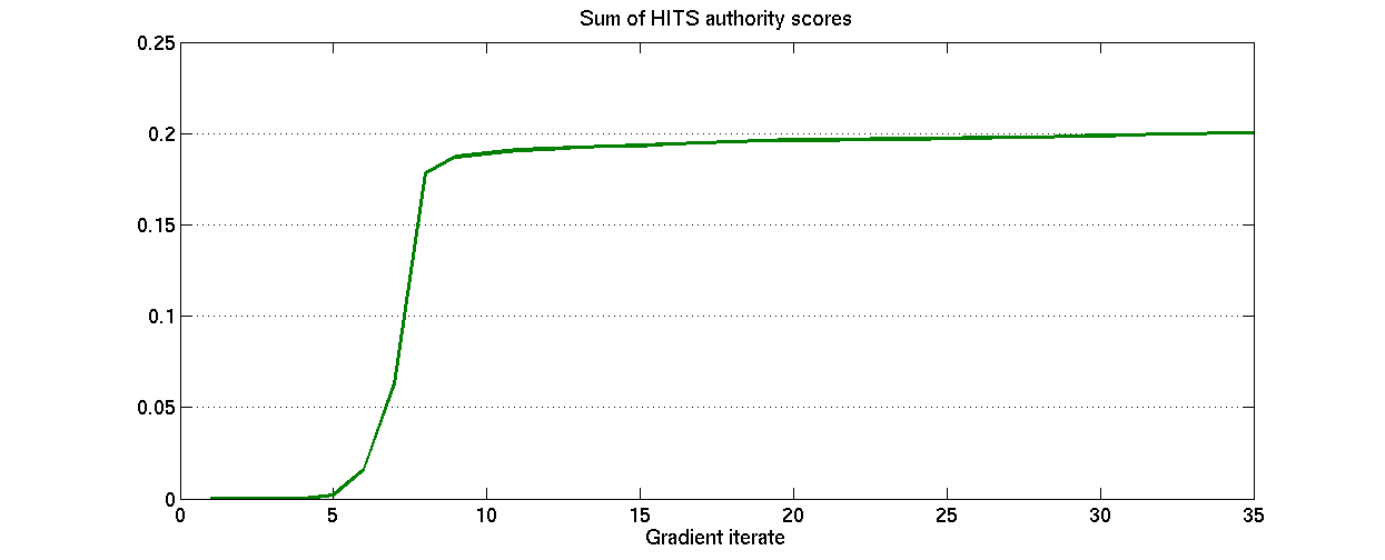
Figure 4: Optimization of the sum of HITS authority scores. The figure shows that the objective is increasing during the course of the algorithm. The sum of authority values jumps from 3.5e-6 to 0.19. However, despite this big progress at the beginning, convergence is slow. This is a typical situation with first order methods and nonconvex optimization.

	Matrix assemblings	Power iterations	Time
Gradient (Equation (4))	545	-	304 s
Gradient (Remark 4)	324	56,239	67 s
Coupled iterations (Th. 2)	589	14,289	15 s

Table 1: Comparison of gradient algorithm with the evaluation of the gradient done by direct resolution of Equation (4) by Matlab “mrdivide” function, gradient algorithm with hot started power iterations described in Remark 4 (precision $10^{-9}$) and coupled gradient and power iterations. The goal was to reach the value 0.22 on our laboratory dataset (the best value we found was 0.2285). For this problem, coupling the power and gradient iterations makes a speedup of more than four.

7.2 HOTS optimization

Here, we cannot use the coupled power and gradient iterations since we do not have any effective bound for the distance between the actual iterate and the true HOTS vector. We thus solve the HOTS optimization problem with classical gradient. We computed the derivative by assuming the conjecture at the end of Section 6.2. Indeed, the second eigenvalue of $\nabla^{2}\theta$ is small while the second eigenvalue of $\mathrm{diag}(d)\nabla^{2}\theta$ is larger. We also never encountered a case where the largest eigenvalue of $\mathrm{diag}(d)\nabla^{2}\theta$ is bigger than 4.

We consider the same website as for the numerical experiments for HITS authority. We take as objective function $f(p)=\sum_{i\in I}\exp(p_{i})$ under the normalization $N(u)=\log(\sum_{i\in[n]}\exp(p_{i}))=0$.

Here, a stationnary point is reached after 55 gradient iterations and 8.2 s. The initial value of the objective was 0.0198 and the final value returned by the optimization algorithm was 0.0567. We give a local optimal adjacency matrix on Figure 5.

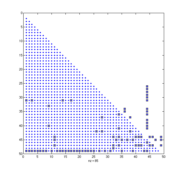
Figure 5: Strict local optimal solution of the HOTS optimization problem. We present the adjacency matrix restricted to the set of controlled pages. There are no facultative external links added. We sorted pages by their $w$ value. The rounded black dots are the obligatory links and the blue dots are the activated facultative links. We can see that the higher the $w$ value, the bigger the number of controlled pages pointing to that page and the smaller the number of pages that page points to (Proposition 12). It is worth noting that this local solution of the relaxed problem has only binary weights.

7.3 Scalability of the algorithms

	HITS (CMAP)	HOTS (CMAP)	HITS (NZU)	HOTS (NZU)
Gradient (Eq. (4))	1.01 s/it	0.82 s/it	out of memory	out of memory
Gradient (Rem. 4)	0.23 s/it	0.12 s/it	20 s/it	62 s/it
Coupled iter. (Th. 2)	0.038 s/it	0.04 s/it	1.0 s/it	2.9 s/it

Table 2: Mean execution times by gradient iterations for HITS authority and HOTS optimization for 2 fragments of the web graph: our laboratory web site and surrounding web pages (CMAP dataset, 1,500 pages) and New Zealand Universities websites (NZU dataset, 413,639 pages). The execution time with a direct resolution of Equation (4) by Matlab “mrdivide” function becomes very memory consuming when the size of the problem grows. It is still acceptable with matrices of size 1,500 but fails for larger matrices. The other two algorithms scale well. For, HOTS optimization problems, as they are not Perron vector optimization problems, Theorem 2 does not apply. However, we have implemented the algorithm anyway. The execution time mainly depends on the spectral gap of the matrix, which is similar in the four cases and on the cost by matrix-vector product, which is growing only linearly thanks to the sparsity of the matrix. The number of gradient iterations is in general not dependent on the size of the problem: in our experiments for HITS authority optimization, there were even less gradient iterations with the larger dataset. When the coupled iterations is available, it gives a speedup between 3 and 20.

We launched our algorithms on two test sets and we give the execution times on Table 2. Our laboratory’s website is described at the beginning of this section. The crawl of New Zealand Universities websites is available at [44]. We selected the 1,696 pages containing the keyword “maori” in their url and 1,807 possible destination pages for the facultative hyperlinks, which yields 3,048,798 facultative hyperlinks. In both cases, we maximize the sum of the scores of the controlled pages.

We remark that for a problem more that 300 times bigger, the computational cost does not increase that much. Indeed, the spectral gap is similar and the cost by matrix-vector product is growing only linearly thanks to the sparsity of the matrix.

References

• AL [06] Konstantin Avrachenkov and Nelly Litvak. The Effect of New Links on Google PageRank. Stochastic Models, 22(2):319–331, 2006.
• BCF+ [11] Frédérique Billy, Jean Clairambault, Olivier Fercoq, Stéphane Gaubert, Thomas Lepoutre, and Thomas Ouillon. Proliferation in cell population models with age structure. In Proceedings of ICNAAM 2011, Kallithea Chalkidis (Greece), pages 1212–1215. American Institute of Physics, 2011.
• Ber [76] Dimitri P. Bertsekas. On the Goldstein - Levitin - Polyak gradient projection method. IEEE transactions on automatic control, AC-21(2):174–184, 1976.
• Ber [95] Dimitri P. Bertsekas. Nonlinear Programming. Athena Scientific, 1995.
• BGLS [06] J.F. Bonnans, J.Ch. Gilbert, C. Lemaréchal, and C. Sagastizábal. Numerical Optimization – Theoretical and Practical Aspects. Universitext. Springer Verlag, Berlin, 2006.
• BP [94] Abraham Berman and Robert J. Plemmons. Nonnegative Matrices in the Mathematical Sciences. Number 9 in Classics in Applied Mathematics. Cambrige University Press, 1994.
• BP [98] Serguey Brin and Larry Page. The anatomy of a large-scale hypertextual web search engine. Computer Networks and ISDN Systems, 30(1-7):107–117, 1998. Proc. 17th International World Wide Web Conference.
• BS [06] Mokhtar S. Bazaraa and Hanif D Sherali. Nonlinear Programming: Theory and Algorithms, 3rd ed. Jon Wiley, New York, 2006.
• BS [07] H. Boche and M. Schubert. Multiuser interference balancing for general interference functions - a convergence analysis. In IEEE International Conference on Communications, pages 4664–4669, 2007.
• BT [00] Vincent D. Blondel and John N. Tsitsiklis. A survey of computational complexity results in systems and control. Automatica, 36(9):1249–1274, 2000.
• BTN [01] Aharon Ben-Tal and Arkadi Nemirovski. Lectures on Modern Convex Optimization, Analysis, Algorithms and Engineering Applications. MPS/SIAM Series on Optimization. SIAM, 2001.
• CDW [75] Jane Cullum, W. E. Donath, and P. Wolfe. The minimization of certain nondifferentiable sums of eigenvalues of symmetric matrices. In Nondifferentiable Optimization, volume 3 of Mathematical Programming Studies, pages 35–55. Springer Berlin Heidelberg, 1975.
• CJB [10] Balázs Csanád Csáji, Raphaël M. Jungers, and Vincent D. Blondel. Pagerank optimization in polynomial time by stochastic shortest path reformulation. In Proc. 21st International Conference on Algorithmic Learning Theory, volume 6331 of Lecture Notes in Computer Science, pages 89–103. Springer, 2010.
• dKNvD [08] Christobald de Kerchove, Laure Ninove, and Paul van Dooren. Maximizing pagerank via outlinks. Linear Algebra and its Applications, 429(5-6):1254–1276, 2008.
• DN [84] Emeric Deutsch and Michael Neumann. Derivatives of the perron root at an essentially nonnegative matrix and the group inverse of an m-matrix. Journal of Mathematical Analysis and Applications, 102(1):1–29, 1984.
• DN [85] Emeric Deutsch and Michael Neumann. On the first and second order derivatives of the perron vector. Linear algebra and its applications, 71:57–76, 1985.
• FABG [10] Olivier Fercoq, Marianne Akian, Mustapha Bouhtou, and Stéphane Gaubert. Ergodic control and polyhedral approaches to Pagerank optimization. arXiv preprint:1011.2348, 2010.
• GB [82] Eli M Gafni and Dimitri P. Bertsekas. Convergence of a gradient projection method. Technical report, LIDS, MIT, 1982.
• GLS [88] Martin Groetschel, László Lovász, and Alexander Schrijver. Geometric Algorithms and Combinatorial Optimization, volume 2 of Algorithms and Combinatorics. Springer-Verlag, 1988.
• HA [89] R. T. Haftka and H. M. Adelman. Recent developments in structural sensitivity analysis. Structural and Multidisciplinary Optimization, 1:137–151, 1989.
• HJ [90] R. A. Horn and C. R. Johnson. Matrix analysis. Cambridge University Press, 1990. Corrected reprint of the 1985 original.
• IT [09] Hideaki Ishii and Roberto Tempo. Computing the pagerank variation for fragile web data. SICE J. of Control, Measurement, and System Integration, 2(1):1–9, 2009.
• Kat [66] Tosio Kato. Perturbation Theory for Linear Operators. Springer-Verlag Berlin and Heidelberg GmbH & Co. K, 1966.
• Kee [93] James P. Keener. The perron-frobenius theorem and the ranking of football teams. SIAM Review, 35(1):80–93, 1993.
• Kin [61] JFC Kingman. A convexity property of positive matrices. The Quarterly Journal of Mathematics, 12(1):283–284, 1961.
• Kle [99] Jon Kleinberg. Authoritative sources in a hyperlinked environment. Journal of the ACM, 46:604–632, 1999.
• LM [00] R. Lempel and S. Moran. The stochastic approach for link-structure analysis (SALSA) and the TKC effect. Computer Networks, 33(1-6):387–401, 2000.
• LM [05] Amy N. Langville and Carl D. Meyer. A survey of eigenvector methods for web information retrieval. SIAM Review, 47(1):135–161, 2005.
• LM [06] Amy N. Langville and Carl D. Meyer. Google’s PageRank and beyond: the science of search engine rankings. Princeton University Press, 2006.
• LO [96] Adrian S. Lewis and Michael L. Overton. Eigenvalue optimization. Acta Numerica, 5:149–190, 1996.
• Log [08] Dmitrii O. Logofet. Convexity in projection matrices: Projection to a calibration problem. Ecological Modelling, 216(2):217–228, 2008.
• Mat [96] Tomomi Matsui. NP-hardness of linear multiplicative programming and related problems. Journal of Global Optimization, 9:113–119, 1996.
• May [94] G. Mayer. Result verification for eigenvectors and eigenvalues. In Proceedings of the IMACS-GAMM international workshop, pages 209–276. Elsevier, 1994.
• MS [88] Carl D. Meyer and G. W. Stewart. Derivatives and perturbations of eigenvectors. SIAM J. on Numerical Analysis, 25(3):679–691, 1988.
• MV [06] Fabien Mathieu and Laurent Viennot. Local aspects of the global ranking of web pages. In 6th International Workshop on Innovative Internet Community Systems (I2CS), pages 1–10, Neuchâtel, 2006.
• Nel [76] R B Nelson. Simplified calculation of eigenvector derivatives. AIAA Journal, 14:1201–1205, 1976.
• NW [99] Jorge Nocedal and Stephen J. Wright. Numerical Optimization. Nueva York, EUA : Springer, 1999.
• Ost [55] Alexander Ostrowski. über normen von matrizen. Mathematische Zeitschrift, 63:2–18, 1955.
• Ove [91] Michael L. Overton. Large-scale optimization of eigenvalues. SIAM J. on Optimization, 2(1):88–120, 1991.
• OW [88] Michael L. Overton and Robert S. Womersley. On minimizing the spectral radius of a nonsymmetric matrix function: optimality conditions and duality theory. SIAM J. on Matrix Analysis and Applications, 9:473–498, 1988.
• Pol [97] Elijah Polak. Optimization: algorithms and consistent approximations. Springer-Verlag New York, 1997.
• PP [73] B. N. Parlett and Jr. Poole, W. G. A geometric theory for the QR, LU and power iterations. SIAM J. on Numerical Analysis, 10(2):389–412, 1973.
• PP [02] Olivier Pironneau and Elijah Polak. Consistent approximations and approximate functions and gradients in optimal control. SIAM J. Control Optim., 41:487–510, 2002.
• Pro [06] Academic Web Link Database Project. New zealand university web sites, January 2006.
• RW [82] Uriel G. Rothblum and Peter Whittle. Growth optimality for branching markov decision chains. Mathematics of Operations Research, 7(4):582–601, 1982.
• Saa [87] Thomas L. Saaty. Rank according to perron: A new insight. Mathematics Magazine, 60(4):211–213, 1987.
• Sch [90] M.H. Schneider. Matrix scaling, entropy minimization and conjugate duality (ii): The dual problem. Math. Prog., 48:103–124, 1990.
• SF [95] Alexander Shapiro and Michael K. H. Fan. On eigenvalue optimization. SIAM J. on Optimization, 5(3):552–569, 1995.
• Tom [03] John A. Tomlin. A new paradigm for ranking pages on the world wide web. In Proc. 12th international conference on World Wide Web, WWW ’03, pages 350–355, New York, 2003. ACM.
• Vig [09] Sebastiano Vigna. Spectral ranking. arXiv preprint:0912.0238, 2009.