Parameter estimation in linear regression driven by a Gaussian sheet

Abstract

The problem of estimating the parameters of a linear regression model  $Z(s,t)=m_{1}g_{1}(s,t)+\cdots+m_{p}g_{p}(s,t)+U(s,t)$   based on observations of  $Z$  on a spatial domain  $G$  of special shape is considered, where the driving process  $U$  is a Gaussian random field and  $g_{1},\ldots,g_{p}$  are known functions. Explicit forms of the maximum-likelihood estimators of the parameters are derived in the cases when  $U$  is either a Wiener or a stationary or nonstationary Ornstein-Uhlenbeck sheet. Simulation results are also presented, where the driving random sheets are simulated with the help of their Karhunen-Loève expansions.

Key words: Wiener sheet, Ornstein-Uhlenbeck sheet, maximum likelihood estimation, Radon-Nikodym derivative.

2010 Mathematics Subject Classifications: 60G60; 62M10; 62M30.

1 Introduction

The Wiener sheet is one of the most important examples of Gaussian random fields. It has various applications in statistical modeling. Wiener sheet appears as limiting process of some random fields defined on the interface of the Ising model (Kuroda and Manaka,, 1987), it is used to model random polymers (Douglas,, 1996), to describe the dynamics of Heath–Jarrow–Morton type forward interest rate models (Goldstein,, 2000) or to model random mortality surfaces (Biffis and Millossovich,, 2006). Further, Carter, (2006) considers the problem of estimation of the mean in a nonparametric regression on a two-dimensional regular grid of design points and constructs a Wiener sheet process on the unit square with a drift that is almost the mean function in the nonparametric regression.

The stationary Ornstein-Uhlenbeck sheet  $\{\widetilde{X}(s,t):s,t\in{\mathbb{R}}\}$  is a zero mean Gaussian process with covariance structure

$${\mathsf{E}}\widetilde{X}(s_{1},t_{1})\widetilde{X}(s_{2},t_{2})=\frac{\sigma^{2}}{4\alpha\beta}{\mathrm{e}}^{-\alpha|s_{2}-s_{1}|-\beta|t_{2}-t_{1}|},$$ (1.1)

where  $\alpha>0$,  $\beta>0$,  $\sigma>0$,  while the random field

$$X(s,t)=\sigma\int\limits_{0}^{s}\int\limits_{0}^{t}{\mathrm{e}}^{\alpha(u-s)+\beta(v-t)}\,{\mathrm{d}}W(u,v),\qquad s,t\geq 0,$$ (1.2)

where  $\alpha\in{\mathbb{R}}$,  $\beta\in{\mathbb{R}}$,  $\sigma>0$  and  $\{W(s,t):s,t\geq 0\}$  is a standard Wiener sheet, can be considered as the Ornstein-Uhlenbeck sheet with zero initial condition on the axes.

Ornstein-Uhlenbeck sheets play role e.g. in potential theory (Feyel and de La Pradelle,, 1995) and, similarly to the Wiener sheet, they also appear as driving fields in forward interest rate models (Goldstein,, 2000; Santa-Clara and Sornette,, 2001).

In this paper we consider a linear regression model driven by a Gaussian sheet, that is a random field

$$Z(s,t):=m_{1}g_{1}(s,t)+\cdots+m_{p}g_{p}(s,t)+U(s,t)$$ (1.3)

observed on a domain  $G$,  where  $g_{1},\ldots,g_{p}$  are known functions and  $U$  is either a Wiener or an Ornstein-Uhlenbeck sheet, and we determine the maximum likelihood estimator (MLE) of the unknown parameters  $m_{1},\ldots,m_{p}$.

In principle, the Radon-Nikodym derivative of Gaussian measures might be derived from the general Feldman-Hajek theorem (Kuo,, 1975), but in most of the cases explicit calculations can not be carried out. In the case when  $U$  is a standard Wiener sheet, $p=1$  and  $g_{1}\equiv 1$  (shifted Wiener sheet),   the MLE of the unknown parameter is given e.g. in Rozanov, (1968), where the estimator is expressed as a function of a usually unknown random variable satisfying some characterizing equation. In several cases the exact form of this random variable can be derived by a method proposed by Rozanov, (1990), based on linear stochastic partial differential equations. Arató, N. M., 1997a used Rozanov’s method to find the MLE of the shift parameter of a shifted Wiener sheet observed on a special domain. Baran et al., (2004) considered the model of Arató, N. M., 1997a , and applying an essentially simpler direct discrete approximation approach the authors found the MLE of the shift parameter under much weaker conditions. Later this discrete approximation was used to determine the MLE of the unknown parameter for the model (1.3) with  $p=1$  and a more complicated domain of observations, when  $U$  is a standard Wiener sheet.

Arató, N. M., 1997b also studied the case when  $U$  is an Ornstein-Uhlenbeck sheet,  $p=1$  and  $g_{1}\equiv 1$,  and using partial stochastic differential equations found the MLE of the unknown parameter based on the observation of the random field  $Z$  on a rectangular domain. This result was generalized by Baran et al., (2003) for the case  $p=1$  and  $g_{1}$  with slight analytic restrictions.

In the present paper we consider the same type of domain  $G$  as in Baran et al., (2011) and extend their result for the general model (1.3). We also consider the cases when the driving process  $U$  is a stationary and a zero start Ornstein-Uhlenbeck sheet and generalize the results of Arató, N. M., 1997b and Baran et al., (2011). Moreover, we present some simulation results to illustrate the theoretical ones where the driving Gaussian random sheets are simulated with the help of their Karhunen-Loève expansions. The proofs of the theorems are given in the Appendix.

2 Models and estimators

Consider the model (1.3) with some given functions  $g_{1},\ldots,g_{p}:{\mathbb{R}}^{2}_{+}\to{\mathbb{R}}$  and with unknown regression parameters  $m_{1},\ldots,m_{p}\in{\mathbb{R}}$.  Let  $[a,c]\subset(0,\infty)$  and  $b_{1},b_{2}\in(a,c)$,  let  $\gamma_{1,2}:[a,b_{1}]\to{\mathbb{R}}$  and  $\gamma_{0}:[b_{2},c]\to{\mathbb{R}}$  be continuous, strictly decreasing functions and let  $\gamma_{1}:[b_{1},c]\to{\mathbb{R}}$  and  $\gamma_{2}:[a,b_{2}]\to{\mathbb{R}}$  be continuous, strictly increasing functions with  $\gamma_{1,2}(b_{1})=\gamma_{1}(b_{1})>0$,  $\gamma_{2}(b_{2})=\gamma_{0}(b_{2})$,  $\gamma_{1,2}(a)=\gamma_{2}(a)$  and  $\gamma_{1}(c)=\gamma_{0}(c)$.   Consider the curve  $\Gamma:=\Gamma_{1,2}\cup\Gamma_{1}\cup\Gamma_{2}\cup\Gamma_{0}$,  where

$$\Gamma_{1,2} :=\Big{\{}\big{(}s,\gamma_{1,2}(s)\big{)}:s\in[a,b_{1}]\Big{\}},\qquad \Gamma_{1}:=\Big{\{}\big{(}s,\gamma_{1}(s)\big{)}:s\in[b_{1},c]\Big{\}},$$

$$\Gamma_{2} :=\Big{\{}\big{(}s,\gamma_{2}(s)\big{)}:s\in[a,b_{2}]\Big{\}}, \Gamma_{0}:=\Big{\{}\big{(}s,\gamma_{0}(s)\big{)}:s\in[b_{2},c]\Big{\}},$$

and for a given  $\varepsilon>0$  let  $\Gamma_{1,2}^{\varepsilon}$,  $\Gamma_{1}^{\varepsilon}$,  $\Gamma_{2}^{\varepsilon}$  and  $\Gamma_{0}^{\varepsilon}$  denote the  inner $\varepsilon$-strip of  $\Gamma_{1,2}$,  $\Gamma_{1}$,  $\Gamma_{2}$  and  $\Gamma_{0}$,  respectively, that is e.g.

$$\Gamma_{1,2}^{\varepsilon}:=\big{\{}(s,t)\in{\mathbb{R}}^{2}:\, s\in[a,a+\varepsilon],\ t\in[\gamma_{1,2}(s),\gamma_{1,2}(a)]\ \text{or}$$

$$s\in[a+\varepsilon,b_{1}],\ t\in[\gamma_{1,2}(s),\gamma_{1,2}(s)+\varepsilon]\big{\}}.$$

Suppose that there exists an  $\varepsilon>0$  such that

$$\Gamma_{1}^{\varepsilon}\cap\Gamma_{2}^{\varepsilon}=\emptyset\quad\text{and}\quad\Gamma_{1,2}^{\varepsilon}\cap\Gamma_{0}^{\varepsilon}=\emptyset,$$ (2.1)

and consider the set  $G:=G_{1}\cup G_{2}\cup G_{3}$,  where

$$G_{1} :=\big{\{}(s,t)\in{\mathbb{R}}^{2}:s\in[a,b_{1}\land b_{2}],\,t\in[\gamma_{1,2}(s),\gamma_{2}(s)]\big{\}},$$

$$G_{2} :=\begin{cases}\big{\{}(s,t)\in{\mathbb{R}}^{2}:s\in[b_{1},b_{2}],\,t\in[\gamma_{1}(s),\gamma_{2}(s)]\big{\}},&\quad\text{if \ $b_{1}\leq b_{2}$,}\\ \big{\{}(s,t)\in{\mathbb{R}}^{2}:s\in[b_{2},b_{1}],\,t\in[\gamma_{1,2}(s),\gamma_{0}(s)]\big{\}},&\quad\text{if \ $b_{1}>b_{2}$,}\end{cases}$$

$$G_{3} :=\big{\{}(s,t)\in{\mathbb{R}}^{2}:s\in[b_{1}\lor b_{2},c],\,t\in[\gamma_{1}(s),\gamma_{0}(s)]\big{\}}.$$

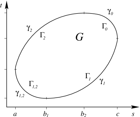
Figure 1: An example of a set of observations  $G$.

An example of such a set of observations can be seen of Figure 1.

First we study the case when  $U$  a standard Wiener sheet and consider the random field  $Z(s,t):=m_{1}g_{1}(s,t)+\cdots+m_{p}g_{p}(s,t)+W(s,t)$.  The following theorem is an obvious extension of Theorem 2.1 of Baran et al., (2011) and can be proved exactly in the same way. The proof is based on the discrete approximation method described in Baran et al., (2003, 2004, 2011), which relies on the results of Arató, (1982, Section 2.3.2).

Theorem 2.1

If  $g_{1},\ldots,g_{p}$  are twice continuously differentiable inside   $G$  and the partial derivatives  $\partial_{1}g_{i},\ \partial_{2}g_{i}$  and  $\partial_{1}\partial_{2}g_{i},\ i=1,\ldots,p$,  can be continuously extended to $G$ then the probability measures  ${\mathsf{P}}_{Z}$  and  ${\mathsf{P}}_{W}$,  generated on  $C(G)$  by the sheets  $Z$  and  $W$,  respectively, are equivalent and the Radon-Nikodym derivative of  ${\mathsf{P}}_{Z}$  with respect to  ${\mathsf{P}}_{W}$  equals

$$\frac{{\mathrm{d}}{\mathsf{P}}_{Z}}{{\mathrm{d}}{\mathsf{P}}_{W}}(Z)=\exp\left\{-\frac{1}{2}\big{(}{\mathbf{m}}^{\top}A{\mathbf{m}}-2\zeta^{\top}{\mathbf{m}}\big{)}\right\},$$

where  $A:=\big{(}A_{k,\ell}\big{)}_{k,\ell=1}^{p}$,  ${\mathbf{m}}:=(m_{1},\ldots,m_{p})^{\top}$  and  $\zeta:=\big{(}\zeta_{1},\ldots,\zeta_{p}\big{)}^{\top}$  with

$$A_{k,\ell}:= \frac{g_{k}\big{(}b_{1},\gamma_{1,2}(b_{1})\big{)}\,g_{\ell}\big{(}b_{1},\gamma_{1,2}(b_{1})\big{)}}{b_{1}\gamma_{1,2}(b_{1})}$$ (2.2)

$$+\int\limits_{a}^{b_{1}}\frac{\big{[}g_{k}\big{(}s,\gamma_{1,2}(s)\big{)}-s\partial_{1}g_{k}\big{(}s,\gamma_{1,2}(s)\big{)}\big{]}\big{[}g_{\ell}\big{(}s,\gamma_{1,2}(s)\big{)}-s\partial_{1}g_{\ell}\big{(}s,\gamma_{1,2}(s)\big{)}\big{]}}{s^{2}\gamma_{1,2}(s)}\,{\mathrm{d}}s$$

$$+\int\limits_{b_{1}}^{c}\frac{\partial_{1}g_{k}\big{(}s,\gamma_{1}(s)\big{)}\,\partial_{1}g_{\ell}\big{(}s,\gamma_{1}(s)\big{)}}{\gamma_{1}(s)}\,{\mathrm{d}}s+\int\limits_{\gamma_{2}(a)}^{\gamma_{2}(b_{2})}\frac{\partial_{2}g_{k}\big{(}\gamma_{2}^{-1}(t),t\big{)}\,\partial_{2}g_{\ell}\big{(}\gamma_{2}^{-1}(t),t\big{)}}{\gamma_{2}^{-1}(t)}\,{\mathrm{d}}t$$

$$+\int\limits_{\gamma_{1,2}(b_{1})}^{\gamma_{1,2}(a)}\frac{\partial_{2}g_{k}\big{(}\gamma_{1,2}^{-1}(t),t\big{)}\,\partial_{2}g_{\ell}\big{(}\gamma_{1,2}^{-1}(t),t\big{)}}{\gamma_{1,2}^{-1}(t)}\,{\mathrm{d}}t+\iint\limits_{G}\partial_{1}\partial_{2}g_{k}(s,t)\,\partial_{1}\partial_{2}g_{\ell}(s,t){\mathrm{d}}s\,{\mathrm{d}}t,$$

and

$$\zeta_{k}:= \frac{g_{k}\big{(}b_{1},\gamma_{1,2}(b_{1})\big{)}Z\big{(}b_{1},\gamma_{1,2}(b_{1})\big{)}}{b_{1}\gamma_{1,2}(b_{1})}+\int\limits_{b_{1}}^{c}\frac{\partial_{1}g_{k}\big{(}s,\gamma_{1}(s)\big{)}}{\gamma_{1}(s)}\,Z\big{(}{\mathrm{d}}s,\gamma_{1}(s)\big{)}$$ (2.3)

$$+\int\limits_{a}^{b_{1}}\frac{\big{[}g_{k}\big{(}s,\gamma_{1,2}(s)\big{)}-s\partial_{1}g_{k}\big{(}s,\gamma_{1,2}(s)\big{)}\big{]}}{s^{2}\gamma_{1,2}(s)}\Big{[}Z\big{(}s,\gamma_{1,2}(s)\big{)}\,{\mathrm{d}}s-sZ\big{(}{\mathrm{d}}s,\gamma_{1,2}(s)\big{)}\Big{]}$$

$$+\int\limits_{\gamma_{2}(a)}^{\gamma_{2}(b_{2})}\frac{\partial_{2}g_{k}\big{(}\gamma_{2}^{-1}(t),t\big{)}}{\gamma_{2}^{-1}(t)}\,Z\big{(}\gamma_{2}^{-1}(t),{\mathrm{d}}t\big{)}+\int\limits_{\gamma_{1,2}(b_{1})}^{\gamma_{1,2}(a)}\frac{\partial_{2}g_{k}\big{(}\gamma_{1,2}^{-1}(t),t\big{)}}{\gamma_{1,2}^{-1}(t)}\,Z\big{(}\gamma_{1,2}^{-1}(t),{\mathrm{d}}t\big{)}$$

$$+\iint\limits_{G}\partial_{1}\partial_{2}g_{k}(s,t)\,Z({\mathrm{d}}s,{\mathrm{d}}t).$$

The maximum likelihood estimator of the parameter vector  ${\mathbf{m}}$  based on the observations  $\{Z(s,t):(s,t)\in G\}$  has the form  ${\widehat{\mathbf{m}}}=A^{-1}\zeta$  and has a $p$-dimensional normal distribution with mean  ${\mathbf{m}}$  and covariance matrix  $A^{-1}$.

Remark 2.2

We remark that the weighted $L^{2}$-Riemann integrals of partial derivatives of the Wiener sheet (and of other $L^{2}$-processes) along a curve are defined in the sense of Baran et al., (2011, Definition 4.1). This means that if  $Z$  is an $L^{2}$-process given along an $\varepsilon$-neighborhood of a curve  $\Gamma:=\big{\{}(s,\gamma(s)):s\in[a,b]\big{\}}$,  where  $\gamma:[a,b]\to{\mathbb{R}}$  is strictly monotone and  $y:[a,b]\to{\mathbb{R}}$  is a function, then

$$\int\limits_{a}^{b}y(s)\,Z({\mathrm{d}}s,\gamma(s)) :=\mathop{\hbox{\rm l.i.m.}}_{h\to 0}\frac{1}{h}\int\limits_{a}^{b}y(s)\big{[}Z(s+h,\gamma(s))-Z(s,\gamma(s))\big{]}\,{\mathrm{d}}s,$$

$$\int\limits_{\gamma(a)}^{\gamma(b)}y(\gamma^{-1}(t))\,Z(\gamma^{-1}(t),{\mathrm{d}}t) :=\mathop{\hbox{\rm l.i.m.}}_{h\to 0}\frac{1}{h}\int\limits_{\gamma(a)}^{\gamma(b)}y(\gamma^{-1}(t))\big{[}Z(\gamma^{-1}(t),t+h)-Z(\gamma^{-1}(t),t)\big{]}\,{\mathrm{d}}t,$$

if the right hand sides exist.

The stationary Ornstein-Uhlenbeck sheet  $\{\widetilde{X}(s,t):s,t\in{\mathbb{R}}\}$  defined by covariance structure (1.1) can be represented as

$$\widetilde{X}(s,t)=\frac{\sigma}{2\sqrt{\alpha\beta}}\,{\mathrm{e}}^{-\alpha s-\beta t}\,W\big{(}{\mathrm{e}}^{2\alpha s},{\mathrm{e}}^{2\beta t}\big{)},\qquad s,t\in{\mathbb{R}}.$$ (2.4)

Consider the sheet  $Z(s,t):=m_{1}h_{1}(s,t)+\cdots+m_{p}h_{p}(s,t)+\widetilde{X}(s,t),\ (s,t)\in{\mathbb{R}}_{+}$.   Applying Theorem 2.1 for the functions

$$g_{k}(u,v)=\frac{2\sqrt{\alpha\beta uv}}{\sigma}\,h_{k}\left(\frac{\log{u}}{2\alpha},\frac{\log{v}}{2\beta}\right),\quad k=1,2,\ldots,p,$$ (2.5)

and for the domain  $\widetilde{G}$  bounded by the curve  $\widetilde{\Gamma}:=\widetilde{\Gamma}_{1,2}\cup\widetilde{\Gamma}_{1}\cup\widetilde{\Gamma}_{2}\cup\widetilde{\Gamma}_{0}$,  where

$$\widetilde{\Gamma}_{1,2} :=\Big{\{}\big{(}u,\widetilde{\gamma}_{1,2}(u)\big{)}:u\in\big{[}{\mathrm{e}}^{2\alpha a},{\mathrm{e}}^{2\alpha b_{1}}\big{]}\Big{\}},\qquad \widetilde{\Gamma}_{1}:=\Big{\{}\big{(}u,\widetilde{\gamma}_{1}(u)\big{)}:u\in\big{[}{\mathrm{e}}^{2\alpha b_{1}},{\mathrm{e}}^{2\alpha c}\big{]}\Big{\}},$$

$$\widetilde{\Gamma}_{2} :=\Big{\{}\big{(}u,\widetilde{\gamma}_{2}(u)\big{)}:u\in\big{[}{\mathrm{e}}^{2\alpha a},{\mathrm{e}}^{2\alpha b_{2}}\big{]}\Big{\}},\qquad \widetilde{\Gamma}_{0}:=\Big{\{}\big{(}u,\widetilde{\gamma}_{0}(u)\big{)}:u\in\big{[}{\mathrm{e}}^{2\alpha b_{2}},{\mathrm{e}}^{2\alpha c}\big{]}\Big{\}},$$

with

$$\widetilde{\gamma}_{j}(u):=\exp\Big{(}2\beta\gamma_{j}\big{(}\log(u)/2\alpha\big{)}\Big{)},\qquad j\in\big{\{}\{1,2\},\{1\},\{2\},\{0\}\big{\}},$$

we obtain the following result.

Theorem 2.3

If  $h_{1},\ldots,h_{p}$  are twice continuously differentiable inside   $G$  and the partial derivatives  $\partial_{1}h_{i},\ \partial_{2}h_{i}$  and  $\partial_{1}\partial_{2}h_{i},\ i=1,\ldots,p$,  can be continuously extended to $G$ then the probability measures  ${\mathsf{P}}_{Z}$  and  ${\mathsf{P}}_{\widetilde{X}}$,  generated on  $C(G)$  by the sheets  $Z$  and  $\widetilde{X}$,  respectively, are equivalent and the Radon-Nikodym derivative of  ${\mathsf{P}}_{Z}$  with respect to  ${\mathsf{P}}_{\widetilde{X}}$  equals

$$\frac{{\mathrm{d}}{\mathsf{P}}_{Z}}{{\mathrm{d}}{\mathsf{P}}_{\widetilde{X}}}(Z)=\exp\left\{-\frac{\alpha\beta}{2\sigma^{2}}\big{(}{\mathbf{m}}^{\top}A{\mathbf{m}}-2\zeta^{\top}{\mathbf{m}}\big{)}\right\},$$

where  $A:=\big{(}A_{k,\ell}\big{)}_{k,\ell=1}^{p}$,  ${\mathbf{m}}:=(m_{1},\ldots,m_{p})^{\top}$  and  $\zeta:=\big{(}\zeta_{1},\ldots,\zeta_{p}\big{)}^{\top}$  with

$$A_{k,\ell}:= \,h_{k}\big{(}a,\gamma_{2}(a)\big{)}h_{\ell}\big{(}a,\gamma_{2}(a)\big{)}+h_{k}\big{(}c,\gamma_{1}(c)\big{)}h_{\ell}\big{(}c,\gamma_{1}(c)\big{)}$$ (2.6)

$$+h_{k}\big{(}b_{1},\gamma_{1}(b_{1})\big{)}h_{\ell}\big{(}b_{1},\gamma_{1}(b_{1})\big{)}+h_{k}\big{(}b_{2},\gamma_{2}(b_{2})\big{)}h_{\ell}\big{(}b_{2},\gamma_{2}(b_{2})\big{)}$$

$$+\int\limits_{a}^{b_{1}}\Big{[}\alpha h_{k}\big{(}s,\gamma_{1,2}(s)\big{)}h_{\ell}\big{(}s,\gamma_{1,2}(s)\big{)}+\alpha^{-1}\partial_{1}h_{k}\big{(}s,\gamma_{1,2}(s)\big{)}\partial_{1}h_{\ell}\big{(}s,\gamma_{1,2}(s)\big{)}\Big{]}\,{\mathrm{d}}s$$

$$+\int\limits_{b_{1}}^{c}\Big{[}\alpha h_{k}\big{(}s,\gamma_{1}(s)\big{)}+\partial_{1}h_{k}\big{(}s,\gamma_{1}(s)\big{)}\Big{]}\Big{[}h_{\ell}\big{(}s,\gamma_{1}(s)\big{)}+\alpha^{-1}\partial_{1}h_{\ell}\big{(}s,\gamma_{1}(s)\big{)}\Big{]}\,{\mathrm{d}}s$$

$$+\int\limits_{a}^{b_{2}}\Big{[}\alpha h_{k}\big{(}s,\gamma_{2}(s)\big{)}-\partial_{1}h_{k}\big{(}s,\gamma_{2}(s)\big{)}\Big{]}\Big{[}h_{\ell}\big{(}s,\gamma_{2}(s)\big{)}-\alpha^{-1}\partial_{1}h_{\ell}\big{(}s,\gamma_{2}(s)\big{)}\Big{]}\,{\mathrm{d}}s$$

$$+\int\limits_{b_{2}}^{c}\Big{[}\alpha h_{k}\big{(}s,\gamma_{0}(s)\big{)}h_{\ell}\big{(}s,\gamma_{0}(s)\big{)}+\alpha^{-1}\partial_{1}h_{k}\big{(}s,\gamma_{0}(s)\big{)}\partial_{1}h_{\ell}\big{(}s,\gamma_{0}(s)\big{)}\Big{]}\,{\mathrm{d}}s$$

$$+\int\limits_{\gamma_{1,2}(b_{1})}^{\gamma_{1,2}(a)}\Big{[}\beta h_{k}\big{(}\gamma_{1,2}^{-1}(t),t\big{)}-\partial_{2}h_{k}\big{(}\gamma_{1,2}^{-1}(t),t\big{)}\Big{]}\Big{[}h_{\ell}\big{(}\gamma_{1,2}^{-1}(t),t\big{)}-\beta^{-1}\partial_{2}h_{\ell}\big{(}\gamma_{1,2}^{-1}(t),t\big{)}\Big{]}\,{\mathrm{d}}t$$

$$+\int\limits_{\gamma_{1}(b_{1})}^{\gamma_{1}(c)}\Big{[}\beta h_{k}\big{(}\gamma_{1}^{-1}(t),t\big{)}h_{\ell}\big{(}\gamma_{1}^{-1}(t),t\big{)}+\beta^{-1}\partial_{2}h_{k}\big{(}\gamma_{1}^{-1}(t),t\big{)}\partial_{2}h_{\ell}\big{(}\gamma_{1}^{-1}(t),t\big{)}\!\Big{]}\,{\mathrm{d}}t$$

$$+\int\limits_{\gamma_{2}(a)}^{\gamma_{2}(b_{2})}\Big{[}\beta h_{k}\big{(}\gamma_{2}^{-1}(t),t\big{)}h_{\ell}\big{(}\gamma_{2}^{-1}(t),t\big{)}+\beta^{-1}\partial_{2}h_{k}\big{(}\gamma_{2}^{-1}(t),t\big{)}\partial_{2}h_{\ell}\big{(}\gamma_{2}^{-1}(t),t\big{)}\Big{]}\,{\mathrm{d}}t$$

$$+\int\limits_{\gamma_{0}(c)}^{\gamma_{0}(b_{2})}\Big{[}\beta h_{k}\big{(}\gamma_{0}^{-1}(t),t\big{)}+\partial_{2}h_{k}\big{(}\gamma_{0}^{-1}(t),t\big{)}\Big{]}\Big{[}h_{\ell}\big{(}\gamma_{0}^{-1}(t),t\big{)}+\beta^{-1}\partial_{2}h_{\ell}\big{(}\gamma_{0}^{-1}(t),t\big{)}\Big{]}\,{\mathrm{d}}t$$

$$+\iint\limits_{G}\big{[}\alpha\beta h_{k}(s,t)h_{\ell}(s,t)+\alpha^{-1}\beta\partial_{1}h_{k}(s,t)\partial_{1}h_{\ell}(s,t)+\alpha\beta^{-1}\partial_{2}h_{k}(s,t)\partial_{2}h_{\ell}(s,t)$$

$$\phantom{+\iint\limits_{G}=}+\alpha^{-1}\beta^{-1}\partial_{1}\partial_{2}h_{k}(s,t)\partial_{1}\partial_{2}h_{\ell}(s,t)\big{]}\,{\mathrm{d}}s\,{\mathrm{d}}t$$

and

$$\zeta_{k}:= \,4h_{k}\big{(}b_{1},\gamma_{1}(b_{1})\big{)}Z\big{(}b_{1},\gamma_{1}(b_{1})\big{)}$$ (2.7)

$$+2\int\limits_{b_{1}}^{c}\Big{[}\alpha h_{k}\big{(}s,\gamma_{1}(s)\big{)}+\partial_{1}h_{k}\big{(}s,\gamma_{1}(s)\big{)}\Big{]}\Big{[}Z\big{(}s,\gamma_{1}(s)\big{)}{\mathrm{d}}s+\alpha^{-1}Z\big{(}{\mathrm{d}}s,\gamma_{1}(s)\big{)}\Big{]}$$

$$+2\int\limits_{a}^{b_{1}}\Big{[}\alpha h_{k}\big{(}s,\gamma_{1,2}(s)\big{)}-\partial_{1}h_{k}\big{(}s,\gamma_{1,2}(s)\big{)}\Big{]}\Big{[}Z\big{(}s,\gamma_{1,2}(s)\big{)}{\mathrm{d}}s-\alpha^{-1}Z\big{(}{\mathrm{d}}s,\gamma_{1,2}(s)\big{)}\Big{]}$$

$$+2\int\limits_{\gamma_{2}(a)}^{\gamma_{2}(b_{2})}\Big{[}\beta h_{k}\big{(}\gamma_{2}^{-1}(t),t\big{)}+\partial_{2}h_{k}\big{(}\gamma_{2}^{-1}(t),t\big{)}\Big{]}\Big{[}Z\big{(}\gamma_{2}^{-1}(t),t\big{)}{\mathrm{d}}t+\beta^{-1}Z\big{(}\gamma_{2}^{-1}(t),{\mathrm{d}}t\big{)}\Big{]}$$

$$+2\int\limits_{\gamma_{1,2}(b_{1})}^{\gamma_{1,2}(a)}\Big{[}\beta h_{k}\big{(}\gamma_{1,2}^{-1}(t),t\big{)}+\partial_{2}h_{k}\big{(}\gamma_{1,2}^{-1}(t),t\big{)}\Big{]}\Big{[}Z\big{(}\gamma_{1,2}^{-1}(t),t\big{)}{\mathrm{d}}t+\beta^{-1}Z\big{(}\gamma_{1,2}^{-1}(t),{\mathrm{d}}t\big{)}\Big{]}$$

$$+\iint\limits_{G}\big{[}\alpha\beta h_{k}(s,t)+\beta\partial_{1}h_{k}(s,t)+\alpha\partial_{2}h_{k}(s,t)+\partial_{1}\partial_{2}h_{k}(s,t)\big{]}$$

$$\phantom{+\iint\limits_{G}=}\times\big{[}Z(s,t){\mathrm{d}}s\,{\mathrm{d}}t+\alpha^{-1}Z({\mathrm{d}}s,t){\mathrm{d}}t+\beta^{-1}Z(s,{\mathrm{d}}t){\mathrm{d}}s+\alpha^{-1}\beta^{-1}Z({\mathrm{d}}s,{\mathrm{d}}t)\big{]}.$$

The maximum likelihood estimator of the parameter vector  ${\mathbf{m}}$  based on the observations  $\{Z(s,t):(s,t)\in G\}$  has the form  ${\widehat{\mathbf{m}}}=A^{-1}\zeta$  and has a $p$-dimensional normal distribution with mean  ${\mathbf{m}}$  and covariance matrix  $A^{-1}$.

Finally, consider the sheet  $Z(s,t):=m_{1}h_{1}(s,t)+\cdots+m_{p}h_{p}(s,t)+X(s,t),\ (s,t)\in{\mathbb{R}}_{+}$, where  $\{X(s,t):s,t\geq 0\}$  is the zero start Ornstein–Uhlenbeck sheet defined by (1.2). For  $\alpha\not=0$  and  $\beta\not=0$  the sheet  $\{X(s,t):s,t\geq 0\}$  can be characterized as a zero mean Gaussian process with

$${\mathsf{E}}X(s_{1},t_{1})X(s_{2},t_{2})=\frac{\sigma^{2}}{4\alpha\beta}\left({\mathrm{e}}^{-\alpha|s_{1}-s_{2}|}-{\mathrm{e}}^{-\alpha(s_{1}+s_{2})}\right)\left({\mathrm{e}}^{-\beta|t_{1}-t_{2}|}-{\mathrm{e}}^{-\beta(t_{1}+t_{2})}\right),$$

hence, for example, in case  $\alpha>0$  and  $\beta>0$  it can also be represented as

$$X(s,t)=\frac{\sigma}{2\sqrt{\alpha\beta}}\,{\mathrm{e}}^{-\alpha s-\beta t}\,W({\mathrm{e}}^{2\alpha s}-1,{\mathrm{e}}^{2\beta t}-1),\qquad s,t\geq 0.$$ (2.8)

In this way similarly to the stationary case one can apply Theorem 2.1 for the functions

$$g_{k}(u,v)=\frac{2\sqrt{\alpha\beta(u+1)(v+1)}}{\sigma}\,h_{k}\left(\frac{\log(u+1)}{2\alpha},\frac{\log(v+1)}{2\beta}\right),\quad k=1,2,\ldots,p,$$ (2.9)

and for the domain  $\widehat{G}$  bounded by the curve  $\widehat{\Gamma}:=\widehat{\Gamma}_{1,2}\cup\widehat{\Gamma}_{1}\cup\widehat{\Gamma}_{2}\cup\widehat{\Gamma}_{0}$,  where

$$\widehat{\Gamma}_{1,2} :=\!\Big{\{}\big{(}u,\widehat{\gamma}_{1,2}(u)\big{)}:u\in\big{[}{\mathrm{e}}^{2\alpha a}\!-\!1,{\mathrm{e}}^{2\alpha b_{1}}\!-\!1\big{]}\Big{\}},\quad \widehat{\Gamma}_{1}:=\!\Big{\{}\big{(}u,\widehat{\gamma}_{1}(u)\big{)}:u\in\big{[}{\mathrm{e}}^{2\alpha b_{1}}\!-\!1,{\mathrm{e}}^{2\alpha c}\!-\!1\big{]}\Big{\}},$$

$$\widehat{\Gamma}_{2} :=\!\Big{\{}\big{(}u,\widehat{\gamma}_{2}(u)\big{)}:u\in\big{[}{\mathrm{e}}^{2\alpha a}\!-\!1,{\mathrm{e}}^{2\alpha b_{2}}\!-\!1\big{]}\Big{\}},\quad \widehat{\Gamma}_{0}:=\!\Big{\{}\big{(}u,\widehat{\gamma}_{0}(u)\big{)}:u\in\big{[}{\mathrm{e}}^{2\alpha b_{2}}\!-\!1,{\mathrm{e}}^{2\alpha c}\!-\!1\big{]}\Big{\}},$$

with

$$\widehat{\gamma}_{j}(u):=\exp\Big{(}2\beta\gamma_{j}\big{(}\log(u+1)/2\alpha\big{)}\Big{)}-1,\qquad j\in\big{\{}\{1,2\},\{1\},\{2\},\{0\}\big{\}},$$

and obtain the following result.

Theorem 2.4

If  $\alpha\not=0$  and  $\beta\not=0$,  functions  $h_{1},\ldots,h_{p}$  are twice continuously differentiable inside   $G$  and the partial derivatives  $\partial_{1}h_{i},\ \partial_{2}h_{i}$  and  $\partial_{1}\partial_{2}h_{i},\ i=1,\ldots,p$,  can be continuously extended to $G$ then the probability measures  ${\mathsf{P}}_{Z}$  and  ${\mathsf{P}}_{X}$,  generated on  $C(G)$  by the sheets  $Z$  and  $X$,  respectively, are equivalent and the Radon-Nikodym derivative of  ${\mathsf{P}}_{Z}$  with respect to  ${\mathsf{P}}_{X}$  equals

$$\frac{{\mathrm{d}}{\mathsf{P}}_{Z}}{{\mathrm{d}}{\mathsf{P}}_{X}}(Z)=\exp\left\{-\frac{\alpha\beta}{2\sigma^{2}}\big{(}{\mathbf{m}}^{\top}A{\mathbf{m}}-2\zeta^{\top}{\mathbf{m}}\big{)}\right\},$$

where  $A:=\big{(}A_{k,\ell}\big{)}_{k,\ell=1}^{p}$,  ${\mathbf{m}}:=(m_{1},\ldots,m_{p})^{\top}$  and  $\zeta:=\big{(}\zeta_{1},\ldots,\zeta_{p}\big{)}^{\top}$  with

$$A_{k,\ell}:\! =\coth\big{(}\alpha a\big{)}\coth\big{(}\beta\gamma_{2}(a)\big{)}h_{k}\big{(}a,\gamma_{2}(a)\big{)}h_{\ell}\big{(}a,\gamma_{2}(a)\big{)}+h_{k}\big{(}c,\gamma_{1}(c)\big{)}h_{\ell}\big{(}c,\gamma_{1}(c)\big{)}$$ (2.10)

$$+\coth\big{(}\beta\gamma_{1}(b_{1})\big{)}h_{k}\big{(}b_{1},\gamma_{1}(b_{1})\big{)}h_{\ell}\big{(}b_{1},\gamma_{1}(b_{1})\big{)}+\coth\big{(}\alpha b_{2}\big{)}h_{k}\big{(}b_{2},\gamma_{2}(b_{2})\big{)}h_{\ell}\big{(}b_{2},\gamma_{2}(b_{2})\big{)}$$

$$+\!\int\limits_{a}^{b_{1}}\!\!\coth\big{(}\beta\gamma_{1,2}(s)\big{)}\!\Big{[}\alpha h_{k}\big{(}s,\gamma_{1,2}(s)\big{)}h_{\ell}\big{(}s,\gamma_{1,2}(s)\big{)}\!+\!\alpha^{-1}\!\partial_{1}h_{k}\big{(}s,\gamma_{1,2}(s)\big{)}\partial_{1}h_{\ell}\big{(}s,\gamma_{1,2}(s)\big{)}\Big{]}{\mathrm{d}}s$$

$$+\int\limits_{b_{1}}^{c}\!\!\coth\big{(}\beta\gamma_{1}(s)\big{)}\Big{[}\alpha h_{k}\big{(}s,\gamma_{1}(s)\big{)}\!+\!\partial_{1}h_{k}\big{(}s,\gamma_{1}(s)\big{)}\Big{]}\Big{[}h_{\ell}\big{(}s,\gamma_{1}(s)\big{)}\!+\!\alpha^{-1}\partial_{1}h_{\ell}\big{(}s,\gamma_{1}(s)\big{)}\Big{]}{\mathrm{d}}s$$

$$+\int\limits_{a}^{b_{2}}\Big{[}\alpha\coth\big{(}\alpha s\big{)}h_{k}\big{(}s,\gamma_{2}(s)\big{)}-\partial_{1}h_{k}\big{(}s,\gamma_{2}(s)\big{)}\Big{]}$$

$$\phantom{+\int\limits_{a}^{b_{2}}}\times\Big{[}\coth\big{(}\alpha s\big{)}h_{\ell}\big{(}s,\gamma_{2}(s)\big{)}-\alpha^{-1}\partial_{1}h_{\ell}\big{(}s,\gamma_{2}(s)\big{)}\Big{]}{\mathrm{d}}s$$

$$+\int\limits_{b_{2}}^{c}\Big{[}\alpha h_{k}\big{(}s,\gamma_{0}(s)\big{)}h_{\ell}\big{(}s,\gamma_{0}(s)\big{)}+\alpha^{-1}\partial_{1}h_{k}\big{(}s,\gamma_{0}(s)\big{)}\partial_{1}h_{\ell}\big{(}s,\gamma_{0}(s)\big{)}\Big{]}{\mathrm{d}}s$$

$$+\int\limits_{\gamma_{1,2}(b_{1})}^{\gamma_{1,2}(a)}\coth\big{(}\alpha\gamma_{1,2}^{-1}(t)\big{)}\Big{[}\beta\coth\big{(}\beta t\big{)}h_{k}\big{(}\gamma_{1,2}^{-1}(t),t\big{)}-\partial_{2}h_{k}\big{(}\gamma_{1,2}^{-1}(t),t\big{)}\Big{]}$$

$$\phantom{===========.}\times\Big{[}\coth\big{(}\beta t\big{)}h_{\ell}\big{(}\gamma_{1,2}^{-1}(t),t\big{)}-\beta^{-1}\partial_{2}h_{\ell}\big{(}\gamma_{1,2}^{-1}(t),t\big{)}\Big{]}{\mathrm{d}}t$$

$$+\int\limits_{\gamma_{1}(b_{1})}^{\gamma_{1}(c)}\Big{[}\beta h_{k}\big{(}\gamma_{1}^{-1}(t),t\big{)}h_{\ell}\big{(}\gamma_{1}^{-1}(t),t\big{)}+\beta^{-1}\partial_{2}h_{k}\big{(}\gamma_{1}^{-1}(t),t\big{)}\partial_{2}h_{\ell}\big{(}\gamma_{1}^{-1}(t),t\big{)}\!\Big{]}{\mathrm{d}}t$$

$$+\!\!\int\limits_{\gamma_{2}(a)}^{\gamma_{2}(b_{2})}\!\!\!\!\coth\big{(}\alpha\gamma_{2}^{-1}(t)\big{)}\!\Big{[}\beta h_{k}\big{(}\gamma_{2}^{-1}(t),t\big{)}h_{\ell}\big{(}\gamma_{2}^{-1}(t),t\big{)}\!+\!\beta^{-1}\partial_{2}h_{k}\big{(}\gamma_{2}^{-1}(t),t\big{)}\partial_{2}h_{\ell}\big{(}\gamma_{2}^{-1}(t),t\big{)}\Big{]}{\mathrm{d}}t$$

$$+\int\limits_{\gamma_{0}(c)}^{\gamma_{0}(b_{2})}\Big{[}\beta h_{k}\big{(}\gamma_{0}^{-1}(t),t\big{)}+\partial_{2}h_{k}\big{(}\gamma_{0}^{-1}(t),t\big{)}\Big{]}\Big{[}h_{\ell}\big{(}\gamma_{0}^{-1}(t),t\big{)}+\beta^{-1}\partial_{2}h_{\ell}\big{(}\gamma_{0}^{-1}(t),t\big{)}\Big{]}{\mathrm{d}}t$$

$$+\iint\limits_{G}\big{[}\alpha\beta h_{k}(s,t)h_{\ell}(s,t)+\alpha^{-1}\beta\partial_{1}h_{k}(s,t)\partial_{1}h_{\ell}(s,t)+\alpha\beta^{-1}\partial_{2}h_{k}(s,t)\partial_{2}h_{\ell}(s,t)$$

$$\phantom{======}+\alpha^{-1}\beta^{-1}\partial_{1}\partial_{2}h_{k}(s,t)\partial_{1}\partial_{2}h_{\ell}(s,t)\big{]}{\mathrm{d}}s\,{\mathrm{d}}t$$

and

$$\zeta_{k}:= \,\Big{[}1+\coth(\alpha b_{1})\Big{]}\Big{[}1+\coth\big{(}\beta\gamma_{1}(b_{1})\big{)}\Big{]}h_{k}\big{(}b_{1},\gamma_{1}(b_{1})\big{)}Z\big{(}b_{1},\gamma_{1}(b_{1})\big{)}$$ (2.11)

$$+\int\limits_{b_{1}}^{c}\Big{[}1+\coth\big{(}\beta\gamma_{1}(s)\big{)}\Big{]}\Big{[}\alpha h_{k}\big{(}s,\gamma_{1}(s)\big{)}+\partial_{1}h_{k}\big{(}s,\gamma_{1}(s)\big{)}\Big{]}$$

$$\phantom{====}\times\Big{[}Z\big{(}s,\gamma_{1}(s)\big{)}{\mathrm{d}}s+\alpha^{-1}Z\big{(}{\mathrm{d}}s,\gamma_{1}(s)\big{)}\Big{]}$$

$$+\int\limits_{a}^{b_{1}}\Big{[}1+\coth\big{(}\beta\gamma_{1,2}(s)\big{)}\Big{]}\Big{[}\alpha\coth(\alpha s)h_{k}\big{(}s,\gamma_{1,2}(s)\big{)}-\partial_{1}h_{k}\big{(}s,\gamma_{1,2}(s)\big{)}\Big{]}$$

$$\phantom{====}\times\Big{[}\coth(\alpha s)Z\big{(}s,\gamma_{1,2}(s)\big{)}{\mathrm{d}}s-\alpha^{-1}Z\big{(}{\mathrm{d}}s,\gamma_{1,2}(s)\big{)}\Big{]}$$

$$+\int\limits_{\gamma_{2}(a)}^{\gamma_{2}(b_{2})}\Big{[}1+\coth\big{(}\alpha\gamma_{2}^{-1}(t)\big{)}\Big{]}\Big{[}\beta h_{k}\big{(}\gamma_{2}^{-1}(t),t\big{)}+\partial_{2}h_{k}\big{(}\gamma_{2}^{-1}(t),t\big{)}\Big{]}$$

$$\phantom{====}\times\Big{[}Z\big{(}\gamma_{2}^{-1}(t),t\big{)}{\mathrm{d}}t+\beta^{-1}Z\big{(}\gamma_{2}^{-1}(t),{\mathrm{d}}t\big{)}\Big{]}$$

$$+\int\limits_{\gamma_{1,2}(b_{1})}^{\gamma_{1,2}(a)}\Big{[}1+\coth\big{(}\alpha\gamma_{1,2}^{-1}(t)\big{)}\Big{]}\Big{[}\beta h_{k}\big{(}\gamma_{1,2}^{-1}(t),t\big{)}+\partial_{2}h_{k}\big{(}\gamma_{1,2}^{-1}(t),t\big{)}\Big{]}$$

$$\phantom{====}\times\Big{[}Z\big{(}\gamma_{1,2}^{-1}(t),t\big{)}{\mathrm{d}}t+\beta^{-1}Z\big{(}\gamma_{1,2}^{-1}(t),{\mathrm{d}}t\big{)}\Big{]}$$

$$+\iint\limits_{G}\big{[}\alpha\beta h_{k}(s,t)+\beta\partial_{1}h_{k}(s,t)+\alpha\partial_{2}h_{k}(s,t)+\partial_{1}\partial_{2}h_{k}(s,t)\big{]}$$

$$\phantom{====}\times\big{[}Z(s,t){\mathrm{d}}s\,{\mathrm{d}}t+\alpha^{-1}Z({\mathrm{d}}s,t){\mathrm{d}}t+\beta^{-1}Z(s,{\mathrm{d}}t){\mathrm{d}}s+\alpha^{-1}\beta^{-1}Z({\mathrm{d}}s,{\mathrm{d}}t)\big{]}.$$

The maximum likelihood estimator of the parameter vector  ${\mathbf{m}}$  based on the observations  $\{Z(s,t):(s,t)\in G\}$  has the form  ${\widehat{\mathbf{m}}}=A^{-1}\zeta$  and has a $p$-dimensional normal distribution with mean  ${\mathbf{m}}$  and covariance matrix  $A^{-1}$.

Remark 2.5

Observe that Theorems 2.1, 2.3 and 2.4 are generalizations of Theorems 4, 5 and 6 of Baran et al., (2003), respectively, where  $G=[S_{1},S_{2}]\times[T_{1},T_{2}]$,  with  $[S_{1},S_{2}],\ [T_{1},T_{2}]\subset(0,\infty)$.   Hence, from these theorems one can also derive the results of Arató, N. M., 1997a ; Arató, N. M., 1997b .

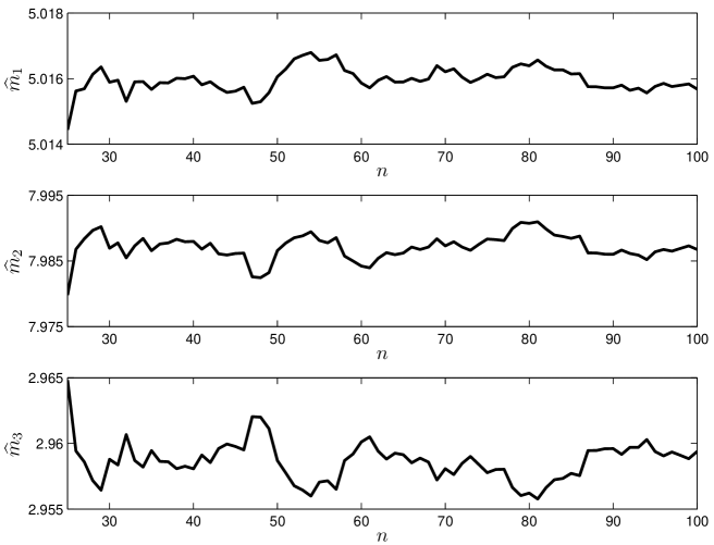
Figure 2: Means of the estimates of the components of  ${\mathbf{m}}$   in Example 3.1 for  $25\leq n\leq 100$.

3 Simulation results

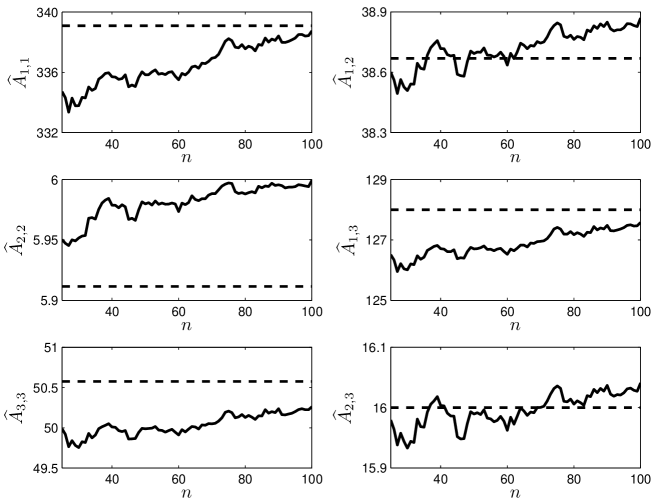
Figure 3: Estimated covariances of  $\zeta$  in Example 3.1 for  $25\leq n\leq 100$.

To illustrate our theoretical results we performed computer simulations using Matlab 2010a. In order to simulate the Gaussian random fields considered above their Karhunen-Loève expansions are applied. For the Wiener sheet  $W(s,t),\ 0\leq s\leq S,\ 0\leq t\leq T$  we have

$$W(s,t)\approx\sum\limits_{j,k=1}^{n}\omega_{j,k}\frac{8\sqrt{ST}}{\pi^{2}(2k-1)(2j-1)}\sin\left(\frac{\pi(2j-1)t}{2T}\right)\sin\left(\frac{\pi(2k-1)s}{2S}\right),$$ (3.1)

where  $\{\omega_{j,k}:1\leq j,k\leq n\}$  are independent standard normal random variables (Deheuvels et al.,, 2006). The expansions for stationary and zero start Ornstein-Uhlenbeck sheets  $\widetilde{X}(s,t)$  and  $X(s,t)$  with  $0\leq s\leq S,\ 0\leq t\leq T$  can directly be derived from (3.1) using representations (2.4) and (2.8), respectively (see e.g. Jaimez and Bonnet, (1987)), yielding

$$\widetilde{X}(s,t)\approx \sum\limits_{j,k=1}^{n}\omega_{j,k}\frac{4\sigma{\mathrm{e}}^{\alpha(S-s)+\beta(T-t)}}{\pi^{2}\sqrt{\alpha\beta}(2k-1)(2j-1)}\sin\left(\frac{\pi(2j-1){\mathrm{e}}^{2\beta(t-T)}}{2}\right)\sin\left(\frac{\pi(2k-1){\mathrm{e}}^{2\alpha(s-S)}}{2}\right),$$

$$X(s,t)\approx \sum\limits_{j,k=1}^{n}\omega_{j,k}\frac{4\sigma\sqrt{({\mathrm{e}}^{2\alpha S}-1)({\mathrm{e}}^{2\beta T}\!-\!1)}}{\pi^{2}{\mathrm{e}}^{\alpha s+\beta t}\sqrt{\alpha\beta}(2k-1)(2j-1)}\sin\left(\frac{\pi(2j-1)({\mathrm{e}}^{2\beta t}-1)}{2({\mathrm{e}}^{2\beta T}-1)}\right)$$

$$\phantom{=====================}\times\sin\left(\frac{\pi(2k-1)({\mathrm{e}}^{2\alpha s}-1)}{2({\mathrm{e}}^{2\alpha S}-1)}\right).$$

In each of the following examples  $1000$  independent samples of the driving Gaussian sheet were simulated with $n$ varying between $25$ and $100$ and the means of the estimates of the parameter vector  ${\mathbf{m}}$  and the empirical covariance matrices of the vectors  $\zeta$  defined by (2.3), (2.7) and (2.11), respectively, were calculated.

Example 3.1

Consider the model

$$Z(s,t)=m_{1}(s^{2}+t^{2})+m_{2}(s+t)+m_{3}(s\cdot t)+W(s,t),\qquad(s,t)\in G,$$

where  $W(s,t),\ (s,t)\in[0,8]^{2}$,  is a standard Wiener sheet and  $G$  is a circle with center at  $(6,6)$  and radius  $r=2$.  In this case the entries of the matrix  $A$  defined by (2.2) and the approximations of the components of  $\zeta=\big{(}\zeta_{1},\zeta_{2},\zeta_{3})^{\top}$  defined by (2.3) can be calculated using numerical integration, where Matlab function quad is applied (recursive adaptive Simpson quadrature).

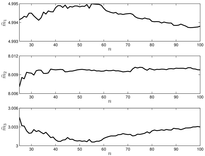
Figure 4: Means of the estimates of the components of  ${\mathbf{m}}$   in Example 3.2 for  $25\leq n\leq 100$.

The theoretical parameter values are  $m_{1}=5,\ m_{2}=8$  and  $m_{3}=3$,  while the theoretical covariance matrix of  $\zeta$  equals

$$A =\begin{pmatrix}339.0895&38.6688&128.0000\\ 38.6688&5.9115&16.0000\\ 128.0000&16.0000&50.5752\end{pmatrix}.$$

On Figure 2 the means of the estimates of the three parameters, while on Figure 3 the estimated covariances of  $\zeta$  are plotted versus the rate  $n$  of the approximation (3.1). In case of  $n=100$  we have  $(5.0157,\ 7.9868,\ 2.9594)$  for the mean and

$$\widehat{A} =\begin{pmatrix}338.7473&38.8697&127.5784\\ 38.8697&5.9995&16.0409\\ 127.5784&16.0409&50.2610\end{pmatrix}$$

for the covariance matrix.

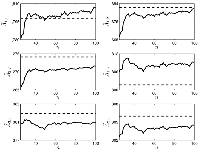
Figure 5: Estimated covariances of  $\zeta$  in Example 3.2 for   $25\leq n\leq 100$.

Example 3.2

Consider the model

$$Z(s,t)=m_{1}(s^{2}+t^{2})+m_{2}(s+t)+m_{3}(s\cdot t)+\widetilde{X}(s,t),\qquad(s,t)\in G,$$

where  $\widetilde{X}(s,t),\ (s,t)\in[0,3]^{2}$,  is a stationary Ornstein-Uhlenbeck sheet with parameters $\alpha=1,\ \beta=1,\ \sigma=1$ and  $G$  is a circle with center at  $(2,2)$  and radius  $r=1$.  Similarly to Example 3.1 the entries of the matrix  $A$  defined by (2.6) and the approximations of the components of  $\zeta=\big{(}\zeta_{1},\zeta_{2},\zeta_{3})^{\top}$  defined by (2.7) can be calculated using numerical integration, where Matlab functions quad and quad2d (Shampine,, 2008) are applied.

The theoretical parameter values are the same as before, that is  $m_{1}=5,\ m_{2}=8$  and  $m_{3}=3$,  while the theoretical covariance matrix of  $\zeta$  equals

$$A =\begin{pmatrix}1797.8554&682.2301&801.6460\\ 682.2301&274.1195&305.9734\\ 801.6460&305.9734&382.9247\end{pmatrix}.$$

On Figure 4 the means of the estimates of the three parameters, while on Figure 5 the estimated covariances of  $\zeta$  are plotted versus the rate  $n$  of the Karhunen-Loève approximation. In case of  $n=100$  we have  $(4.9938,\ 8.0098,\ 3.0030)$  for the mean and

$$\widehat{A} =\begin{pmatrix}1806.4240&681.5420&809.0529\\ 681.5420&271.5779&304.4110\\ 809.0529&304.4110&380.8634\end{pmatrix}$$

for the covariance matrix.

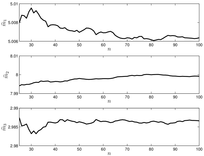
Figure 6: Means of the estimates of the components of  ${\mathbf{m}}$  in Example 3.3 for  $25\leq n\leq 100$.

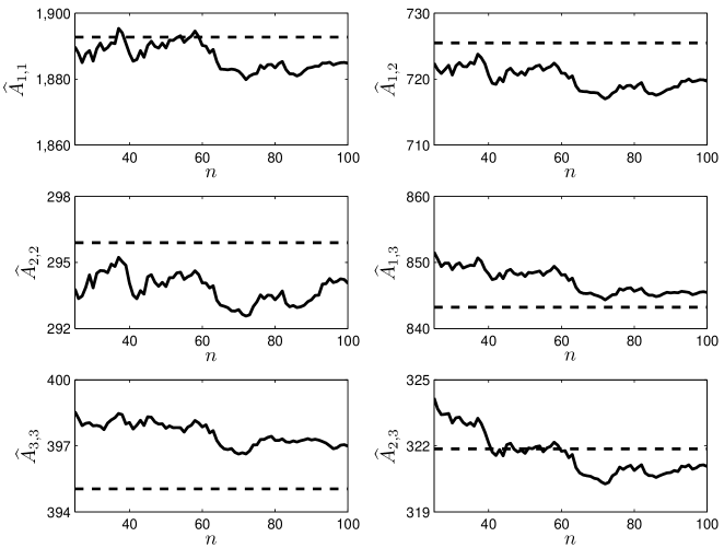
Figure 7: Estimated covariances of  $\zeta$  in Example 3.3 for  $25\leq n\leq 100$.

Example 3.3

Consider the same regression

$$Z(s,t)=m_{1}(s^{2}+t^{2})+m_{2}(s+t)+m_{3}(s\cdot t)+X(s,t),\qquad(s,t)\in G,$$

as in Examples 3.1 and 3.2, but now the driving process  $X(s,t),\ (s,t)\in[0,3]^{2}$,  is a zero start Ornstein-Uhlenbeck sheet with parameters $\alpha=1,\ \beta=1,\ \sigma=1$.  Similarly to Example 3.2,  $G$  is a circle with center at  $(2,2)$  and radius  $r=1$.  Again, the entries of the matrix  $A$  defined by (2.10) and the approximations of the components of  $\zeta=\big{(}\zeta_{1},\zeta_{2},\zeta_{3})^{\top}$  defined by (2.11) can only be calculated with the help of numerical integration.

The theoretical parameter values are the same as before, that is  $m_{1}=5,\ m_{2}=8$  and  $m_{3}=3$,  while the theoretical covariance matrix of  $\zeta$  equals

$$A =\begin{pmatrix}1892.7035&725.4822&843.2301\\ 725.4822&295.8952&321.8680\\ 843.2301&321.8680&395.0477\end{pmatrix}.$$

Similarly to the previous examples, on Figure 6 the means of the estimates of the three parameters, while on Figure 7 the estimated covariances of  $\zeta$  are plotted versus the rate  $n$  of the Karhunen-Loève approximation. In case of  $n=100$  we have  $(5.0067,\ 7.9992,\ 2.9866)$  for the mean and

$$\widehat{A} =\begin{pmatrix}1884.8293&719.6687&845.4606\\ 719.6687&294.0491&321.0663\\ 840.0300&321.0663&396.9913\end{pmatrix}$$

for the covariance matrix.

Appendix A Appendix

A.1 Proof of Theorem 2.3

To prove Theorem 2.3 one has to use representation (2.4) and apply Theorem 2.1 for the random field

$$Y(u,v):=\frac{2\sqrt{\alpha\beta uv}}{\sigma}Z\Big{(}\frac{\log u}{2\alpha},\frac{\log v}{2\beta}\Big{)}=m_{1}g_{1}(u,v)+\ldots+m_{p}g_{p}(u,v)+W(u,v)$$

observed on  $\widetilde{G}$,  where functions  $g_{k}$  are defined by (2.5). As

$$\partial_{1}g_{k}(u,v) =\frac{\sqrt{\beta v}}{\sigma\sqrt{\alpha u}}(\alpha+\partial_{1})h_{k}\Big{(}\frac{\log u}{2\alpha},\frac{\log v}{2\beta}\Big{)},$$

$$\partial_{2}g_{k}(u,v) =\frac{\sqrt{\alpha u}}{\sigma\sqrt{\beta v}}(\beta+\partial_{2})h_{k}\Big{(}\frac{\log u}{2\alpha},\frac{\log v}{2\beta}\Big{)},$$ (A.1)

$$\partial_{1}\partial_{2}g_{k}(u,v) =\frac{1}{2\sigma\sqrt{\alpha\beta uv}}(\alpha+\partial_{1})(\beta+\partial_{2})h_{k}\Big{(}\frac{\log u}{2\alpha},\frac{\log v}{2\beta}\Big{)},$$

short calculations show

$$A_{k,\ell}= \,4h_{k}\big{(}b_{1},\gamma_{1,2}(b_{1})\big{)}\,h_{\ell}\big{(}b_{1},\gamma_{1,2}(b_{1})\big{)}$$

$$+2\int\limits_{a}^{b_{1}}\Big{[}(\alpha-\partial_{1})h_{k}\big{(}s,\gamma_{1,2}(s)\big{)}\Big{]}\Big{[}(1-\alpha^{-1}\partial_{1})h_{\ell}\big{(}s,\gamma_{1,2}(s)\big{)}\Big{]}\,{\mathrm{d}}s$$

$$+2\int\limits_{b_{1}}^{c}\Big{[}(\alpha+\partial_{1})h_{k}\big{(}s,\gamma_{1}(s)\big{)}\Big{]}\Big{[}(1+\alpha^{-1}\partial_{1})h_{\ell}\big{(}s,\gamma_{1}(s)\big{)}\Big{]}\,{\mathrm{d}}s$$

$$+2\int\limits_{\gamma_{2}(a)}^{\gamma_{2}(b_{2})}\Big{[}(\beta+\partial_{2})h_{k}\big{(}\gamma_{2}^{-1}(t),t\big{)}\Big{]}\Big{[}(1+\beta^{-1}\partial_{2})h_{\ell}\big{(}\gamma_{2}^{-1}(t),t\big{)}\Big{]}\,{\mathrm{d}}t$$

$$+2\int\limits_{\gamma_{1,2}(b_{1})}^{\gamma_{1,2}(a)}\Big{[}(\beta+\partial_{2})h_{k}\big{(}\gamma_{1,2}^{-1}(t),t\big{)}\Big{]}\Big{[}(1+\beta^{-1}\partial_{2})h_{\ell}\big{(}\gamma_{1,2}^{-1}(t),t\big{)}\Big{]}\,{\mathrm{d}}t$$

$$+\iint\limits_{G}\Big{[}(\alpha+\partial_{1})(\beta+\partial_{2})h_{k}(s,t)\Big{]}\Big{[}(1+\alpha^{-1}\partial_{1})(1+\beta^{-1}\partial_{2})h_{\ell}(s,t)\Big{]}\,{\mathrm{d}}s\,{\mathrm{d}}t$$

$$= A_{k,\ell}^{(1)}+\alpha A_{k,\ell}^{(2)}+\beta A_{k,\ell}^{(3)}+\alpha^{-1}A_{k,\ell}^{(4)}+\beta^{-1}A_{k,\ell}^{(5)}+A_{k,\ell}^{(6)},$$

where

$$A_{k,\ell}^{(1)}:= \,4h_{k}\big{(}b_{1},\gamma_{1,2}(b_{1})h_{\ell}\big{(}b_{1},\gamma_{1,2}(b_{1})\big{)}+2\int\limits_{b_{1}}^{c}\partial_{1}\Big{[}h_{k}\big{(}s,\gamma_{1}(s)\big{)}h_{\ell}\big{(}s,\gamma_{1}(s)\big{)}\Big{]}\,{\mathrm{d}}s$$

$$-2\int\limits_{a}^{b_{1}}\partial_{1}\Big{[}h_{k}\big{(}s,\gamma_{1,2}(s)\big{)}h_{\ell}\big{(}s,\gamma_{1,2}(s)\big{)}\Big{]}\,{\mathrm{d}}s+2\int\limits_{\gamma_{2}(a)}^{\gamma_{2}(b_{2})}\partial_{2}\Big{[}h_{k}\big{(}\gamma_{2}^{-1}(t),t\big{)}h_{\ell}\big{(}\gamma_{2}^{-1}(t),t\big{)}\Big{]}\,{\mathrm{d}}t$$

$$+2\int\limits_{\gamma_{1,2}(b_{1})}^{\gamma_{1,2}(a)}\partial_{2}\Big{[}h_{k}\big{(}\gamma_{1,2}^{-1}(t),t\big{)}h_{\ell}\big{(}\gamma_{1,2}^{-1}(t),t\big{)}\Big{]}\,{\mathrm{d}}t+\iint\limits_{G}\partial_{1}\partial_{2}\big{[}h_{k}(s,t)h_{\ell}(s,t)\big{]}\,{\mathrm{d}}s\,{\mathrm{d}}t,$$

$$A_{k,\ell}^{(2)}:= \,2\int\limits_{b_{1}}^{c}h_{k}\big{(}s,\gamma_{1}(s)\big{)}h_{\ell}\big{(}s,\gamma_{1}(s)\big{)}\,{\mathrm{d}}s+2\int\limits_{a}^{b_{1}}h_{k}\big{(}s,\gamma_{1,2}(s)\big{)}h_{\ell}\big{(}s,\gamma_{1,2}(s)\big{)}\,{\mathrm{d}}s$$

$$+\iint\limits_{G}\partial_{2}\big{[}h_{k}(s,t)h_{\ell}(s,t)\big{]}\,{\mathrm{d}}s\,{\mathrm{d}}t,$$

$$A_{k,\ell}^{(3)}:= 2\int\limits_{\gamma_{2}(a)}^{\gamma_{2}(b_{2})}h_{k}\big{(}\gamma_{2}^{-1}(t),t\big{)}h_{\ell}\big{(}\gamma_{2}^{-1}(t),t\big{)}\,{\mathrm{d}}t+2\int\limits_{\gamma_{1,2}(b_{1})}^{\gamma_{1,2}(a)}h_{k}\big{(}\gamma_{1,2}^{-1}(t),t\big{)}h_{\ell}\big{(}\gamma_{1,2}^{-1}(t),t\big{)}\,{\mathrm{d}}t$$

$$+\iint\limits_{G}\partial_{1}\big{[}h_{k}(s,t)h_{\ell}(s,t)\big{]}\,{\mathrm{d}}s\,{\mathrm{d}}t,$$

$$A_{k,\ell}^{(4)}:= \,2\int\limits_{b_{1}}^{c}\partial_{1}h_{k}\big{(}s,\gamma_{1}(s)\big{)}\,\partial_{1}h_{\ell}\big{(}s,\gamma_{1}(s)\big{)}\,{\mathrm{d}}s+2\int\limits_{a}^{b_{1}}\partial_{1}h_{k}\big{(}s,\gamma_{1,2}(s)\big{)}\,\partial_{1}h_{\ell}\big{(}s,\gamma_{1,2}(s)\big{)}\,{\mathrm{d}}s$$

$$+\iint\limits_{G}\partial_{2}\big{[}\partial_{1}h_{k}(s,t)\,\partial_{1}h_{\ell}(s,t)\big{]}\,{\mathrm{d}}s\,{\mathrm{d}}t,$$

$$A_{k,\ell}^{(5)}:= 2\int\limits_{\gamma_{2}(a)}^{\gamma_{2}(b_{1})}\partial_{2}h_{k}\big{(}\gamma_{2}^{-1}(t),t\big{)}\,\partial_{2}h_{\ell}\big{(}\gamma_{2}^{-1}(t),t\big{)}\,{\mathrm{d}}t+2\int\limits_{\gamma_{1,2}(b_{1})}^{\gamma_{1,2}(a)}\partial_{2}h_{k}\big{(}\gamma_{1,2}^{-1}(t),t\big{)}\,\partial_{2}h_{\ell}\big{(}\gamma_{1,2}^{-1}(t),t\big{)}\,{\mathrm{d}}t$$

$$+\iint\limits_{G}\partial_{1}\big{[}\partial_{2}h_{k}(s,t)\,\partial_{2}h_{\ell}(s,t)\big{]}\,{\mathrm{d}}s\,{\mathrm{d}}t,$$

$$A_{k,\ell}^{(6)}:= \iint\limits_{G}\big{[}\alpha\beta h_{k}(s,t)h_{\ell}(s,t)+\alpha^{-1}\beta\partial_{1}h_{k}(s,t)\partial_{1}h_{\ell}(s,t)+\alpha\beta^{-1}\partial_{2}h_{k}(s,t)\partial_{2}h_{\ell}(s,t)$$

$$\phantom{+\iint\limits_{G}=}+\alpha^{-1}\beta^{-1}\partial_{1}\partial_{2}h_{k}(s,t)\partial_{1}\partial_{2}h_{\ell}(s,t)\big{]}\,{\mathrm{d}}s\,{\mathrm{d}}t.$$

Obviously

$$\iint\limits_{G}\partial_{2}\big{[}h_{k}(s,t) \,h_{\ell}(s,t)\big{]}{\mathrm{d}}s\,{\mathrm{d}}t=\!\int\limits_{a}^{b_{2}}\!h_{k}\big{(}s,\gamma_{2}(s)\big{)}h_{\ell}\big{(}s,\gamma_{2}(s)\big{)}\,{\mathrm{d}}s-\!\int\limits_{a}^{b_{1}}\!h_{k}\big{(}s,\gamma_{1,2}(s)\big{)}h_{\ell}\big{(}s,\gamma_{1,2}(s)\big{)}\,{\mathrm{d}}s$$

$$-\!\int\limits_{b_{1}}^{c}\!h_{k}\big{(}s,\gamma_{1}(s)\big{)}h_{\ell}\big{(}s,\gamma_{1}(s)\big{)}\,{\mathrm{d}}s+\!\int\limits_{b_{2}}^{c}\!h_{k}\big{(}s,\gamma_{0}(s)\big{)}h_{\ell}\big{(}s,\gamma_{0}(s)\big{)}\,{\mathrm{d}}s,$$ (A.2)

$$\iint\limits_{G}\partial_{1}\big{[}h_{k}(s,t) \,h_{\ell}(s,t)\big{]}{\mathrm{d}}s\,{\mathrm{d}}t=\!\!\!\int\limits_{\gamma_{1}(b_{1})}^{\gamma_{1}(c)}\!\!\!h_{k}\big{(}\gamma_{1}^{-1}(t),t\big{)}h_{\ell}\big{(}\gamma_{1}^{-1}(t),t\big{)}\,{\mathrm{d}}t-\!\!\!\!\!\!\int\limits_{\gamma_{1,2}(b_{1})}^{\gamma_{1,2}(a)}\!\!\!\!\!h_{k}\big{(}\gamma_{1,2}^{-1}(t),t\big{)}h_{\ell}\big{(}\gamma_{1,2}^{-1}(t),t\big{)}\,{\mathrm{d}}t$$

$$-\!\!\int\limits_{\gamma_{2}(a)}^{\gamma_{2}(b_{2})}\!\!h_{k}\big{(}\gamma_{2}^{-1}(t),t\big{)}h_{\ell}\big{(}\gamma_{2}^{-1}(t),t\big{)}\,{\mathrm{d}}t+\!\!\!\int\limits_{\gamma_{0}(c)}^{\gamma_{0}(b_{2})}\!\!h_{k}\big{(}\gamma_{0}^{-1}(t),t\big{)}h_{\ell}\big{(}\gamma_{0}^{-1}(t),t\big{)}\,{\mathrm{d}}t,$$ (A.3)

and similar expressions can be derived for

$$\iint\limits_{G}\partial_{2}\big{[}\partial_{1}h_{k}(s,t)\,\partial_{1}h_{\ell}(s,t)\big{]}\,{\mathrm{d}}s\,{\mathrm{d}}t\qquad\text{and}\qquad\iint\limits_{G}\partial_{1}\big{[}\partial_{2}h_{k}(s,t)\,\partial_{2}h_{\ell}(s,t)\big{]}\,{\mathrm{d}}s\,{\mathrm{d}}t,$$

respectively. Hence, using also that

$$2\iint\limits_{G} \partial_{1}\partial_{2}\big{[}h_{k}(s,t)h_{\ell}(s,t)\big{]}\,{\mathrm{d}}s\,{\mathrm{d}}t$$ (A.4)

$$= \int\limits_{a}^{b_{2}}\partial_{1}\Big{[}h_{k}\big{(}s,\gamma_{2}(s)\big{)}h_{\ell}\big{(}s,\gamma_{2}(s)\big{)}\Big{]}\,{\mathrm{d}}s-\int\limits_{\gamma_{2}(a)}^{\gamma_{2}(b_{2})}\partial_{2}\Big{[}h_{k}\big{(}\gamma_{2}^{-1}(t),t\big{)}h_{\ell}\big{(}\gamma_{2}^{-1}(t),t\big{)}\Big{]}\,{\mathrm{d}}t$$

$$-\int\limits_{b_{1}}^{c}\partial_{1}\Big{[}h_{k}\big{(}s,\gamma_{1}(s)\big{)}h_{\ell}\big{(}s,\gamma_{1}(s)\big{)}\Big{]}\,{\mathrm{d}}s+\int\limits_{\gamma_{1}(b_{1})}^{\gamma_{1}(c)}\partial_{2}\Big{[}h_{k}\big{(}\gamma_{1}^{-1}(t),t\big{)}h_{\ell}\big{(}\gamma_{1}^{-1}(t),t\big{)}\Big{]}\,{\mathrm{d}}t$$

$$-\int\limits_{a}^{b_{1}}\partial_{1}\Big{[}h_{k}\big{(}s,\gamma_{1,2}(s)\big{)}h_{\ell}\big{(}s,\gamma_{1,2}(s)\big{)}\Big{]}\,{\mathrm{d}}s+\int\limits_{\gamma_{1,2}(a)}^{\gamma_{1,2}(b_{1})}\partial_{2}\Big{[}h_{k}\big{(}\gamma_{1,2}^{-1}(t),t\big{)}h_{\ell}\big{(}\gamma_{1,2}^{-1}(t),t\big{)}\Big{]}\,{\mathrm{d}}t$$

$$+\int\limits_{b_{2}}^{c}\partial_{1}\Big{[}h_{k}\big{(}s,\gamma_{0}(s)\big{)}h_{\ell}\big{(}s,\gamma_{0}(s)\big{)}\Big{]}\,{\mathrm{d}}s-\int\limits_{\gamma_{0}(b_{2})}^{\gamma_{0}(c)}\partial_{2}\Big{[}h_{k}\big{(}\gamma_{0}^{-1}(t),t\big{)}h_{\ell}\big{(}\gamma_{0}^{-1}(t),t\big{)}\Big{]}\,{\mathrm{d}}t,$$

after tedious but straightforward calculations we obtain (2.6).

Further, using again (A.1) and Remark 2.2 we have

$$\zeta_{k}=\zeta_{k}^{(1)}+\zeta_{k}^{(2)}+\zeta_{k}^{(3)}+\zeta_{k}^{(4)}+\zeta_{k}^{(5)}+\zeta_{k}^{(6)},$$

where

$$\zeta_{k}^{(1)}:= \,4h_{k}\big{(}b_{1},\gamma_{1,2}(b_{1})\big{)}Z\big{(}b_{1},\gamma_{1,2}(b_{1})\big{)}$$

$$\zeta_{k}^{(2)}:= \,\mathop{\hbox{\rm l.i.m.}}_{\varrho\to 0}\frac{4}{\varrho}\int\limits_{b_{1}}^{c}{\mathrm{e}}^{\alpha s}(\alpha+\partial_{1})h_{k}\big{(}s,\gamma_{1}(s)\big{)}$$

$$\phantom{\,\mathop{\hbox{\rm l.i.m.}}_{\varrho\to 0}\frac{1}{\varrho}\int\limits_{b_{1}}^{c}}\times\bigg{[}\big{(}{\mathrm{e}}^{2\alpha s}+\varrho\big{)}^{1/2}Z\Big{(}\frac{\log({\mathrm{e}}^{2\alpha s}+\varrho)}{2\alpha},\gamma_{1}(s)\Big{)}-{\mathrm{e}}^{\alpha s}Z\big{(}s,\gamma_{1}(s)\big{)}\bigg{]}\,{\mathrm{d}}s,$$

$$\zeta_{k}^{(3)}:= \,4\int\limits_{a}^{b_{1}}\big{(}\alpha-\partial_{1}\big{)}h_{k}\big{(}s,\gamma_{1,2}(s)\big{)}Z\big{(}s,\gamma_{1,2}(s)\big{)}{\mathrm{d}}s$$

$$-\mathop{\hbox{\rm l.i.m.}}_{\varrho\to 0}\frac{4}{\varrho}\int\limits_{a}^{b_{1}}{\mathrm{e}}^{\alpha s}(\alpha-\partial_{1})h_{k}\big{(}s,\gamma_{1,2}(s)\big{)}$$

$$\phantom{\,\mathop{\hbox{\rm l.i.m.}}_{\varrho\to 0}\frac{1}{\varrho}\int\limits_{a}^{b_{1}}}\times\bigg{[}\big{(}{\mathrm{e}}^{2\alpha s}+\varrho\big{)}^{1/2}Z\Big{(}\frac{\log({\mathrm{e}}^{2\alpha s}+\varrho)}{2\alpha},\gamma_{1,2}(s)\Big{)}-{\mathrm{e}}^{\alpha s}Z\big{(}s,\gamma_{1,2}(s)\big{)}\bigg{]}\,{\mathrm{d}}s,$$

$$\zeta_{k}^{(4)}:= \,\mathop{\hbox{\rm l.i.m.}}_{\delta\to 0}\frac{4}{\delta}\int\limits_{\gamma_{2}(a)}^{\gamma_{2}(b_{2})}{\mathrm{e}}^{\beta t}(\beta+\partial_{2})h_{k}\big{(}\gamma_{2}^{-1}(t),t\big{)}$$

$$\phantom{\,\mathop{\hbox{\rm l.i.m.}}_{\varrho\to 0}\frac{1}{\varrho}\int\limits_{\gamma_{2}(a)}^{\gamma_{2}(b_{2})}}\times\bigg{[}\big{(}{\mathrm{e}}^{2\beta t}+\delta\big{)}^{1/2}Z\Big{(}\gamma_{2}^{-1}(t),\frac{\log({\mathrm{e}}^{2\beta t}+\delta)}{2\beta}\Big{)}-{\mathrm{e}}^{\beta t}Z\big{(}\gamma_{2}^{-1}(t),t\big{)}\bigg{]}\,{\mathrm{d}}t,$$

$$\zeta_{k}^{(5)}:= \,\mathop{\hbox{\rm l.i.m.}}_{\delta\to 0}\frac{4}{\delta}\int\limits_{\gamma_{1,2}(b_{1})}^{\gamma_{1,2}(a)}{\mathrm{e}}^{\beta t}(\beta+\partial_{2})h_{k}\big{(}\gamma_{1,2}^{-1}(t),t\big{)}$$

$$\phantom{\,\mathop{\hbox{\rm l.i.m.}}_{\varrho\to 0}\frac{1}{\varrho}\int\limits_{\gamma_{1,2}(b_{1})}^{\gamma_{1,2}(1)}}\times\bigg{[}\big{(}{\mathrm{e}}^{2\beta t}+\delta\big{)}^{1/2}Z\Big{(}\gamma_{1,2}^{-1}(t),\frac{\log({\mathrm{e}}^{2\beta t}+\delta)}{2\beta}\Big{)}-{\mathrm{e}}^{\beta t}Z\big{(}\gamma_{1,2}^{-1}(t),t\big{)}\bigg{]}\,{\mathrm{d}}t,$$

$$\zeta_{k}^{(6)}:= \,\mathop{\hbox{\rm l.i.m.}}_{\varrho,\delta\to 0}\frac{4}{\varrho\delta}\iint\limits_{G}{\mathrm{e}}^{\alpha s+\beta t}(\alpha+\partial_{1})(\beta+\partial_{2})h_{k}\big{(}s,t\big{)}\bigg{[}{\mathrm{e}}^{\alpha s+\beta t}Z(s,t)$$

$$\phantom{,\mathop{\hbox{\rm l.i.m.}}_{\varrho,\delta\to 0}\frac{4}{\varrho\delta}\iint\limits_{G}}-\!\big{(}{\mathrm{e}}^{2\alpha s}\!+\!\varrho\big{)}^{1/2}{\mathrm{e}}^{\beta t}Z\Big{(}\frac{\log({\mathrm{e}}^{2\alpha s}\!+\!\varrho)}{2\alpha},t\Big{)}\!-\!{\mathrm{e}}^{\alpha s}\big{(}{\mathrm{e}}^{2\beta t}\!+\!\delta\big{)}^{1/2}Z\Big{(}s,\frac{\log({\mathrm{e}}^{2\beta t}\!+\!\delta)}{2\beta}\Big{)}$$

$$\phantom{,\mathop{\hbox{\rm l.i.m.}}_{\varrho,\delta\to 0}\frac{4}{\varrho\delta}\iint\limits_{G}}+\!\big{(}{\mathrm{e}}^{2\alpha s}+\varrho\big{)}^{1/2}\big{(}{\mathrm{e}}^{2\beta t}+\delta\big{)}^{1/2}Z\Big{(}\frac{\log({\mathrm{e}}^{2\alpha s}+\varrho)}{2\alpha},\frac{\log({\mathrm{e}}^{2\beta t}+\delta)}{2\beta}\Big{)}\bigg{]}{\mathrm{d}}s\,{\mathrm{d}}t,$$

implying (2.7). $\square$

A.2 Proof of Theorem 2.4

The proof, which we give only in the case  $\alpha>0,\ \beta>0$,  is similar to the proof of Theorem 2.3. Here one has to use representation (2.8) and apply Theorem 2.1 for the random field

$$Y(u,v):= \,\frac{2\sqrt{\alpha\beta(u+1)(v+1)}}{\sigma}Z\Big{(}\frac{\log(u+1)}{2\alpha},\frac{\log(v+1)}{2\beta}\Big{)}$$

$$= \,m_{1}g_{1}(u,v)+\ldots+m_{p}g_{p}(u,v)+W(u,v)$$

observed on  $\widehat{G}$,  and functions  $g_{k}$  should be defined by (2.9). In this way

$$\partial_{1}g_{k}(u,v) =\frac{\sqrt{\beta(v+1)}}{\sigma\sqrt{\alpha(u+1)}}(\alpha+\partial_{1})h_{k}\Big{(}\frac{\log(u+1)}{2\alpha},\frac{\log(v+1)}{2\beta}\Big{)},$$

$$\partial_{2}g_{k}(u,v) =\frac{\sqrt{\alpha(u+1)}}{\sigma\sqrt{\beta(v+1)}}(\beta+\partial_{2})h_{k}\Big{(}\frac{\log(u+1)}{2\alpha},\frac{\log(v+1)}{2\beta}\Big{)},$$ (A.5)

$$\partial_{1}\partial_{2}g_{k}(u,v) =\frac{1}{2\sigma\sqrt{\alpha\beta(u+1)(v+1)}}(\alpha+\partial_{1})(\beta+\partial_{2})h_{k}\Big{(}\frac{\log(u+1)}{2\alpha},\frac{\log(v+1)}{2\beta}\Big{)},$$

so

$$A_{k,\ell}=\,4\frac{{\mathrm{e}}^{2\alpha b_{1}}}{{\mathrm{e}}^{2\alpha b_{1}}-1}\frac{{\mathrm{e}}^{2\beta\gamma_{1,2}(b_{1})}}{{\mathrm{e}}^{2\beta\gamma_{1,2}(b_{1})}-1}h_{k}\big{(}b_{1},\gamma_{1,2}(b_{1})\big{)}\,h_{\ell}\big{(}b_{1},\gamma_{1,2}(b_{1})\big{)}$$

$$\phantom{=}+2\!\int\limits_{a}^{b_{1}}\!\frac{{\mathrm{e}}^{2\beta\gamma_{1,2}(s)}}{{\mathrm{e}}^{2\beta\gamma_{1,2}(s)}\!-\!1}\Big{[}\big{(}\alpha\coth(\alpha s)\!-\!\partial_{1}\big{)}h_{k}\big{(}s,\gamma_{1,2}(s)\big{)}\Big{]}\Big{[}\big{(}\coth(\alpha s)\!-\!\alpha^{-1}\partial_{1}\big{)}h_{\ell}\big{(}s,\gamma_{1,2}(s)\big{)}\Big{]}\,{\mathrm{d}}s$$

$$\phantom{=}+2\int\limits_{b_{1}}^{c}\frac{{\mathrm{e}}^{2\beta\gamma_{1}(s)}}{{\mathrm{e}}^{2\beta\gamma_{1}(s)}\!-\!1}\Big{[}(\alpha+\partial_{1})h_{k}\big{(}s,\gamma_{1}(s)\big{)}\Big{]}\Big{[}(1+\alpha^{-1}\partial_{1})h_{\ell}\big{(}s,\gamma_{1}(s)\big{)}\Big{]}\,{\mathrm{d}}s$$

$$\phantom{=}+2\int\limits_{\gamma_{2}(a)}^{\gamma_{2}(b_{2})}\frac{{\mathrm{e}}^{2\alpha\gamma_{2}^{-1}(t)}}{{\mathrm{e}}^{2\alpha\gamma_{2}^{-1}(t)}\!-\!1}\Big{[}(\beta+\partial_{2})h_{k}\big{(}\gamma_{2}^{-1}(t),t\big{)}\Big{]}\Big{[}(1+\beta^{-1}\partial_{2})h_{\ell}\big{(}\gamma_{2}^{-1}(t),t\big{)}\Big{]}\,{\mathrm{d}}t$$

$$\phantom{=}+2\int\limits_{\gamma_{1,2}(b_{1})}^{\gamma_{1,2}(a)}\frac{{\mathrm{e}}^{2\alpha\gamma_{1,2}^{-1}(t)}}{{\mathrm{e}}^{2\alpha\gamma_{1,2}^{-1}(t)}\!-\!1}\Big{[}(\beta+\partial_{2})h_{k}\big{(}\gamma_{1,2}^{-1}(t),t\big{)}\Big{]}\Big{[}(1+\beta^{-1}\partial_{2})h_{\ell}\big{(}\gamma_{1,2}^{-1}(t),t\big{)}\Big{]}\,{\mathrm{d}}t$$

$$\phantom{=}+\iint\limits_{G}\Big{[}(\alpha+\partial_{1})(\beta+\partial_{2})h_{k}(s,t)\Big{]}\Big{[}(1+\alpha^{-1}\partial_{1})(1+\beta^{-1}\partial_{2})h_{\ell}(s,t)\Big{]}\,{\mathrm{d}}s\,{\mathrm{d}}t.$$

Collecting separately the terms containing  $\gamma_{1,2},\ \gamma_{1},\ \gamma_{2}$  and  $\gamma_{0}$,  after long straightforward calculations using again (A.2)–(A.4) we obtain

$$A_{k,\ell}=A_{k,\ell}^{(1)}+A_{k,\ell}^{(2)}+A_{k,\ell}^{(3)}+A_{k,\ell}^{(4)}+A_{k,\ell}^{(5)},$$

where

$$A_{k,\ell}^{(1)}:= \,\frac{1}{2}h_{k}\big{(}b_{1},\gamma_{1,2}(b_{1})\big{)}h_{\ell}\big{(}b_{1},\gamma_{1,2}(b_{1})\big{)}-\frac{1}{2}h_{k}\big{(}a,\gamma_{1,2}(a)\big{)}h_{\ell}\big{(}a,\gamma_{1,2}(a)\big{)}$$

$$+\coth\big{(}\alpha a\big{)}\coth\big{(}\beta\gamma_{1,2}(a)\big{)}h_{k}\big{(}a,\gamma_{1,2}(a)\big{)}h_{\ell}\big{(}a,\gamma_{1,2}(a)\big{)}$$

$$+\coth\big{(}\beta\gamma_{1,2}(b_{1})\big{)}h_{k}\big{(}b_{1},\gamma_{1,2}(b_{1})\big{)}h_{\ell}\big{(}b_{1},\gamma_{1,2}(b_{1})\big{)}+\coth\big{(}\alpha a\big{)}h_{k}\big{(}a,\gamma_{1,2}(a)\big{)}h_{\ell}\big{(}a,\gamma_{1,2}(a)\big{)}$$

$$+\int\limits_{a}^{b_{1}}\coth\big{(}\beta\gamma_{1,2}(s)\big{)}\Big{[}\alpha h_{k}\big{(}s,\gamma_{1,2}(s)\big{)}h_{\ell}\big{(}s,\gamma_{1,2}(s)\big{)}+\alpha^{-1}\partial_{1}h_{k}\big{(}s,\gamma_{1,2}(s)\big{)}\partial_{1}h_{\ell}\big{(}s,\gamma_{1,2}(s)\big{)}\Big{]}{\mathrm{d}}s$$

$$+\int\limits_{\gamma_{1,2}(b_{1})}^{\gamma_{1,2}(a)}\coth\big{(}\alpha\gamma_{1,2}^{-1}(t)\big{)}\Big{[}\big{(}\beta\coth(\beta t)-\partial_{2}\big{)}h_{k}\big{(}\gamma_{1,2}^{-1}(t),t\big{)}\Big{]}$$

$$\phantom{============}\times\Big{[}\big{(}\coth(\beta t)-\beta^{-1}\partial_{2}\big{)}h_{\ell}\big{(}\gamma_{1,2}^{-1}(t),t\big{)}\Big{]}{\mathrm{d}}t,$$

$$A_{k,\ell}^{(2)}:= \,\frac{1}{2}h_{k}\big{(}c,\gamma_{1}(c)\big{)}h_{\ell}\big{(}c,\gamma_{1}(c)\big{)}-\frac{1}{2}h_{k}\big{(}b_{1},\gamma_{1}(b_{1})\big{)}h_{\ell}\big{(}b_{1},\gamma_{1}(b_{1})\big{)}$$

$$+\int\limits_{b_{1}}^{c}\coth\big{(}\beta\gamma_{1}(s)\big{)}\Big{[}\big{(}\alpha+\partial_{1}\big{)}h_{k}\big{(}s,\gamma_{1}(s)\big{)}\Big{]}\Big{[}\big{(}1+\alpha^{-1}\partial_{1}\big{)}h_{\ell}\big{(}s,\gamma_{1}(s)\big{)}\Big{]}{\mathrm{d}}s$$

$$+\int\limits_{\gamma_{1}(b_{1})}^{\gamma_{1}(c)}\Big{[}\beta h_{k}\big{(}\gamma_{1}^{-1}(t),t\big{)}h_{\ell}\big{(}\gamma_{1}^{-1}(t),t\big{)}+\beta^{-1}\partial_{2}h_{k}\big{(}\gamma_{1}^{-1}(t),t\big{)}\partial_{2}h_{\ell}\big{(}\gamma_{1}^{-1}(t),t\big{)}\Big{]}{\mathrm{d}}t,$$

$$A_{k,\ell}^{(3)}:= \,\frac{1}{2}h_{k}\big{(}b_{2},\gamma_{2}(b_{2})\big{)}h_{\ell}\big{(}b_{2},\gamma_{2}(b_{2})\big{)}-\frac{1}{2}h_{k}\big{(}a,\gamma_{2}(a)\big{)}h_{\ell}\big{(}a,\gamma_{2}(a)\big{)}$$

$$+\coth\big{(}\alpha b_{2}\big{)}h_{k}\big{(}b_{2},\gamma_{2}(b_{2})\big{)}h_{\ell}\big{(}b_{2},\gamma_{2}(b_{2})\big{)}-\coth\big{(}\alpha a\big{)}h_{k}\big{(}a,\gamma_{2}(a)\big{)}h_{\ell}\big{(}a,\gamma_{2}(a)\big{)}$$

$$+\int\limits_{a}^{b_{2}}\Big{[}\big{(}\alpha\coth(\alpha s)-\partial_{1}\big{)}h_{k}\big{(}s,\gamma_{2}(s)\big{)}\Big{]}\Big{[}\big{(}\coth(\alpha s)-\alpha^{-1}\partial_{1}\big{)}h_{\ell}\big{(}s,\gamma_{2}(s)\big{)}\Big{]}{\mathrm{d}}s$$

$$+\!\!\!\!\!\int\limits_{\gamma_{2}(a)}^{\gamma_{2}(b_{2})}\!\!\!\!\coth\big{(}\alpha\gamma_{2}^{-1}(t)\big{)}\Big{[}\beta h_{k}\big{(}\gamma_{2}^{-1}(t),t\big{)}h_{\ell}\big{(}\gamma_{2}^{-1}(t),t\big{)}+\beta^{-1}\partial_{2}h_{k}\big{(}\gamma_{2}^{-1}(t),t\big{)}\partial_{2}h_{\ell}\big{(}\gamma_{2}^{-1}(t),t\big{)}\Big{]}{\mathrm{d}}t,$$

$$A_{k,\ell}^{(4)}:= \frac{1}{2}h_{k}\big{(}c,\gamma_{0}(c)\big{)}h_{\ell}\big{(}c,\gamma_{0}(c)\big{)}-\frac{1}{2}h_{k}\big{(}b_{2},\gamma_{0}(b_{2})\big{)}h_{\ell}\big{(}b_{2},\gamma_{0}(b_{2})\big{)}$$

$$+\int\limits_{b_{2}}^{c}\Big{[}\alpha h_{k}\big{(}s,\gamma_{0}(s)\big{)}h_{\ell}\big{(}s,\gamma_{0}(s)\big{)}+\alpha^{-1}\partial_{1}h_{k}\big{(}s,\gamma_{0}(s)\big{)}\partial_{1}h_{\ell}\big{(}s,\gamma_{0}(s)\big{)}\Big{]}{\mathrm{d}}s$$

$$+\int\limits_{\gamma_{0}(c)}^{\gamma_{0}(b_{2})}\Big{[}\big{(}\beta+\partial_{2}\big{)}h_{k}\big{(}\gamma_{0}^{-1}(t),t\big{)}\Big{]}\Big{[}\big{(}1+\beta^{-1}\partial_{2}\big{)}h_{\ell}\big{(}\gamma_{0}^{-1}(t),t\big{)}\Big{]}{\mathrm{d}}t,$$

$$A_{k,\ell}^{(5)}:= \iint\limits_{G}\big{[}\alpha\beta h_{k}(s,t)h_{\ell}(s,t)+\alpha^{-1}\beta\partial_{1}h_{k}(s,t)\partial_{1}h_{\ell}(s,t)+\alpha\beta^{-1}\partial_{2}h_{k}(s,t)\partial_{2}h_{\ell}(s,t)$$

$$\phantom{+\iint\limits_{G}=}+\alpha^{-1}\beta^{-1}\partial_{1}\partial_{2}h_{k}(s,t)\partial_{1}\partial_{2}h_{\ell}(s,t)\big{]}\,{\mathrm{d}}s\,{\mathrm{d}}t,$$

which equals (2.10).

At the end, using again (A.5) and Remark 2.2 we have

$$\zeta_{k}=\zeta_{k}^{(1)}+\zeta_{k}^{(2)}+\zeta_{k}^{(3)}+\zeta_{k}^{(4)}+\zeta_{k}^{(5)}+\zeta_{k}^{(6)},$$

where

$$\zeta_{k}^{(1)}:= \,\frac{4{\mathrm{e}}^{2\alpha b_{1}+2\beta\gamma_{1,2}(b_{1})}}{({\mathrm{e}}^{2\alpha b_{1}}-1)({\mathrm{e}}^{2\beta\gamma_{1,2}(b_{1})}-1)}h_{k}\big{(}b_{1},\gamma_{1,2}(b_{1})\big{)}Z\big{(}b_{1},\gamma_{1,2}(b_{1})\big{)}$$

$$\zeta_{k}^{(2)}:= \,\mathop{\hbox{\rm l.i.m.}}_{\varrho\to 0}\frac{1}{\varrho}\int\limits_{b_{1}}^{c}\frac{4{\mathrm{e}}^{\alpha s+2\beta\gamma_{1}(s)}}{{\mathrm{e}}^{2\beta\gamma_{1}(s)}-1}(\alpha+\partial_{1})h_{k}\big{(}s,\gamma_{1}(s)\big{)}$$

$$\phantom{\,\mathop{\hbox{\rm l.i.m.}}_{\varrho\to 0}\frac{1}{\varrho}\int\limits_{b_{1}}^{c}}\times\bigg{[}\big{(}{\mathrm{e}}^{2\alpha s}+\varrho\big{)}^{1/2}Z\Big{(}\frac{\log({\mathrm{e}}^{2\alpha s}+\varrho)}{2\alpha},\gamma_{1}(s)\Big{)}-{\mathrm{e}}^{\alpha s}Z\big{(}s,\gamma_{1}(s)\big{)}\bigg{]}\,{\mathrm{d}}s,$$

$$\zeta_{k}^{(3)}:= \,\int\limits_{a}^{b_{1}}\frac{4{\mathrm{e}}^{2\alpha s+2\beta\gamma_{1,2}(s)}}{({\mathrm{e}}^{2\alpha s}-1)({\mathrm{e}}^{2\beta\gamma_{1,2}(s)}-1)}\big{(}\alpha\coth(\alpha s)-\partial_{1}\big{)}h_{k}\big{(}s,\gamma_{1,2}(s)\big{)}Z\big{(}s,\gamma_{1,2}(s)\big{)}{\mathrm{d}}s$$

$$-\mathop{\hbox{\rm l.i.m.}}_{\varrho\to 0}\frac{1}{\varrho}\int\limits_{a}^{b_{1}}\frac{4{\mathrm{e}}^{\alpha s+2\beta\gamma_{1,2}(s)}}{{\mathrm{e}}^{2\beta\gamma_{1,2}(s)}-1}\big{(}\alpha\coth(\alpha s)-\partial_{1})h_{k}\big{(}s,\gamma_{1,2}(s)\big{)}$$

$$\phantom{\,\mathop{\hbox{\rm l.i.m.}}_{\varrho\to 0}\frac{1}{\varrho}\int\limits_{a}^{b_{1}}}\times\bigg{[}\big{(}{\mathrm{e}}^{2\alpha s}+\varrho\big{)}^{1/2}Z\Big{(}\frac{\log({\mathrm{e}}^{2\alpha s}+\varrho)}{2\alpha},\gamma_{1,2}(s)\Big{)}-{\mathrm{e}}^{\alpha s}Z\big{(}s,\gamma_{1,2}(s)\big{)}\bigg{]}\,{\mathrm{d}}s,$$

$$\zeta_{k}^{(4)}:= \,\mathop{\hbox{\rm l.i.m.}}_{\delta\to 0}\frac{1}{\delta}\int\limits_{\gamma_{2}(a)}^{\gamma_{2}(b_{2})}\frac{4{\mathrm{e}}^{\beta t+2\alpha\gamma_{2}^{-1}(t)}}{{\mathrm{e}}^{2\alpha\gamma_{2}^{-1}(t)}-1}(\beta+\partial_{2})h_{k}\big{(}\gamma_{2}^{-1}(t),t\big{)}$$

$$\phantom{\,\mathop{\hbox{\rm l.i.m.}}_{\varrho\to 0}\frac{1}{\varrho}\int\limits_{\gamma_{2}(a)}^{\gamma_{2}(b_{2})}}\times\bigg{[}\big{(}{\mathrm{e}}^{2\beta t}+\delta\big{)}^{1/2}Z\Big{(}\gamma_{2}^{-1}(t),\frac{\log({\mathrm{e}}^{2\beta t}+\delta)}{2\beta}\Big{)}-{\mathrm{e}}^{\beta t}Z\big{(}\gamma_{2}^{-1}(t),t\big{)}\bigg{]}\,{\mathrm{d}}t,$$

$$\zeta_{k}^{(5)}:= \,\mathop{\hbox{\rm l.i.m.}}_{\delta\to 0}\frac{1}{\delta}\int\limits_{\gamma_{1,2}(b_{1})}^{\gamma_{1,2}(a)}\frac{4{\mathrm{e}}^{\beta t+2\alpha\gamma_{1,2}^{-1}(t)}}{{\mathrm{e}}^{2\alpha\gamma_{1,2}^{-1}(t)}-1}(\beta+\partial_{2})h_{k}\big{(}\gamma_{1,2}^{-1}(t),t\big{)}$$

$$\phantom{\,\mathop{\hbox{\rm l.i.m.}}_{\varrho\to 0}\frac{1}{\varrho}\int\limits_{\gamma_{1,2}(b_{1})}^{\gamma_{1,2}(1)}}\times\bigg{[}\big{(}{\mathrm{e}}^{2\beta t}+\delta\big{)}^{1/2}Z\Big{(}\gamma_{1,2}^{-1}(t),\frac{\log({\mathrm{e}}^{2\beta t}+\delta)}{2\beta}\Big{)}-{\mathrm{e}}^{\beta t}Z\big{(}\gamma_{1,2}^{-1}(t),t\big{)}\bigg{]}\,{\mathrm{d}}t,$$

$$\zeta_{k}^{(6)}:= \,\mathop{\hbox{\rm l.i.m.}}_{\varrho,\delta\to 0}\frac{4}{\varrho\delta}\iint\limits_{G}{\mathrm{e}}^{\alpha s+\beta t}(\alpha+\partial_{1})(\beta+\partial_{2})h_{k}\big{(}s,t\big{)}\bigg{[}{\mathrm{e}}^{\alpha s+\beta t}Z(s,t)$$

$$\phantom{,\mathop{\hbox{\rm l.i.m.}}_{\varrho,\delta\to 0}\frac{4}{\varrho\delta}\iint\limits_{G}}-\!\big{(}{\mathrm{e}}^{2\alpha s}\!+\!\varrho\big{)}^{1/2}{\mathrm{e}}^{\beta t}Z\Big{(}\frac{\log({\mathrm{e}}^{2\alpha s}\!+\!\varrho)}{2\alpha},t\Big{)}\!-\!{\mathrm{e}}^{\alpha s}\big{(}{\mathrm{e}}^{2\beta t}\!+\!\delta\big{)}^{1/2}Z\Big{(}s,\frac{\log({\mathrm{e}}^{2\beta t}\!+\!\delta)}{2\beta}\Big{)}$$

$$\phantom{,\mathop{\hbox{\rm l.i.m.}}_{\varrho,\delta\to 0}\frac{4}{\varrho\delta}\iint\limits_{G}}+\!\big{(}{\mathrm{e}}^{2\alpha s}+\varrho\big{)}^{1/2}\big{(}{\mathrm{e}}^{2\beta t}+\delta\big{)}^{1/2}Z\Big{(}\frac{\log({\mathrm{e}}^{2\alpha s}+\varrho)}{2\alpha},\frac{\log({\mathrm{e}}^{2\beta t}+\delta)}{2\beta}\Big{)}\bigg{]}{\mathrm{d}}s\,{\mathrm{d}}t,$$

implying (2.11). $\square$

Acknowledgments.  Research has been supported by the Hungarian Scientific Research Fund under Grant No. OTKA T079128/2009 and partially supported by TÁMOP 4.2.1./B-09/1/KONV-2010-0007/IK/IT project. The project is implemented through the New Hungary Development Plan co-financed by the European Social Fund, and the European Regional Development Fund.

References

Arató, (1982)
Arató, M. (1982) Linear stochastic systems with
constant coefficients. A statistical approach. Springer-Verlag,
Berlin; in Russian: Nauka, Moscow, 1989.
(2)
Arató, N. M. (1997a) Mean estimation of Brownian sheet. Comput. Math. Appl.33, no. 8, 13–25.
(3)