Lattice Determination of the Anomalous Magnetic Moment of the Muon

Abstract:

a MKPH-T-11-21
a HIM-2011-11
a CERN-PH-TH-2011-280

We compute the leading hadronic contribution to the anomalous magnetic moment of the muon $a_{\mu}^{\mathrm{HLO}}$ using two dynamical flavours of non-perturbatively $\mathcal{O}(a)$ improved Wilson fermions. By applying partially twisted boundary conditions we are able to improve the momentum resolution of the vacuum polarisation, an important ingredient for the determination of the leading hadronic contribution. We check systematic uncertainties by studying several ensembles, which allows us to discuss finite size effects and lattice artefacts. The chiral behavior of $a_{\mu}^{\mathrm{HLO}}$ turns out to be non-trivial, especially for small pion masses.

1 Introduction

The anomalous magnetic moment of the muon is defined as half the difference between the gyromagnetic factor of the muon $g_{\mu}$ and 2: $a_{\mu}=(g_{\mu}-2)/2$. This quantity is commonly used to test the Standard Model of particle physics, since it can be measured and computed to a very high precision. Currently a discrepancy of $3.2$ standard deviations between experiment and theory is observed [1], which might be a hint for physics beyond the Standard Model. The hadronic contributions, especially the hadronic vacuum polarisation $a_{\mu}^{\mathrm{HLO}}$, dominate the theoretical uncertainties. Currently the Standard Model prediction of $a_{\mu}^{\mathrm{HLO}}$ is determined using the optical theorem to relate the cross-section $e^{+}e^{-}\,\rightarrow\,\mathit{hadrons}$ data to the vacuum polarisation. A calculation from first principles is clearly desirable. Here we report on our current effort towards a precise determination of the leading hadronic contribution to the anomalous magnetic moment of the muon using Lattice QCD.

2 Lattice Setup

$\beta$	$a$ $[\mathrm{fm}]$	lattice	$L$ $[\mathrm{fm}]$	$m_{\pi}$ $[\mathrm{MeV}]$	$m_{\pi}L$	Labels
$5.20$	$0.079$	$64\times 32^{3}$	$2.5$	$471$ - $317$	$6.0$ - $4.0$	A3 - A5
$5.30$	$0.063$	$64\times 32^{3}$	$2.0$	$644$ - $447$	$7.9$ - $4.7$	E3 - E5
$5.30$	$0.063$	$96\times 48^{3}$	$3.0$	$323$, $277$	$5.0$, $4.2$	F6, F7
$5.50$	$0.050$	$96\times 48^{3}$	$2.4$	$541$, $431$	$6.5$, $5.2$	N4, N5

Table 1: Summary of simulations parameters. Measurements are performed on configurations separated by $8$ units of molecular dynamics time at least. The scale and pion masses are still preliminary and taken from [10,11].

We use two dynamical flavours of non-perturbatively $\mathcal{O}(a)$ improved Wilson fermions [2] and include a partially quenched strange quark. Similar studies have been performed in the quenched approximation [3,4] and in the theory with two [5,6] and three dynamical flavours [7,8]. Our measurements are performed on a subset of the gauge configurations generated as part of the CLS project [9]. The simulations parameters are listed in Table 1. On the lattice the vacuum polarisation tensor is defined by a Fourier-transformation of a current-current correlator

$$\Pi_{\mu\nu}(q)=a^{4}\sum_{x}e^{iq(x+a\hat{\mu}/2-a\hat{\nu}/2)}\left<J^{\mathrm{c}}_{\mu}(x)J^{\mathrm{c}}_{\nu}(0)\right>,$$ (1)

where we use the conserved point-split current $J^{\mathrm{c}}_{\mu}(x)$ [4] given in the case of Wilson fermions by

$$J^{\mathrm{c}}_{\mu}(x)=\frac{1}{2}\bigg{(}\bar{q}(x+a\hat{\mu})(1+\gamma_{\mu})U_{\mu}^{+}(x)q(x)-\bar{q}(x)(1-\gamma_{\mu})U_{\mu}(x)q(x+a\hat{\mu})\bigg{)}.$$ (2)

Preforming the Wick contractions in Equation 1 produces connected as well as disconnected contributions. Disconnected diagrams are computationally expensive and neglected in this study. Nevertheless two-flavour chiral perturbation theory of NLO allows us to estimate the disconnected contributions to be $-10\%$ of the connected one [12].

Current conservation implies that the vacuum polarisation tensor $\Pi_{\mu\nu}(q)$ can be related to the vacuum polarisation $\Pi(q^{2})$ in the following way:

$$\Pi_{\mu\nu}(q)=\left(\delta_{\mu\nu}q^{2}-q_{\mu}q_{\nu}\right)\Pi(q^{2}).$$ (3)

For space-like momenta, the relation between the vacuum polarisation $\Pi(q^{2})$ and the lowest order hadronic contribution to the anomalous magnetic moment of the muon $a_{\mu}^{\mathrm{HLO}}$ has been derived in [3,4,13]

$$a_{\mu}=\left(\frac{\alpha}{\pi}\right)^{2}\int_{0}^{\infty}dq^{2}\,f(q^{2})\hat{\Pi}(q^{2}),$$ (4)

where the kernel of this integral is given by

$$f(q^{2})=\frac{m_{\mu}^{2}q^{2}Z^{3}(1-q^{2}Z)}{1+m_{\mu}^{2}q^{2}Z^{2}},\qquad Z=\frac{q^{2}-\sqrt{q^{4}-4m_{\mu}^{2}q^{2}}}{2m_{\mu}^{2}q^{2}}$$ (5)

and $\hat{\Pi}(q^{2})=4\pi\left(\Pi(q^{2})-\Pi(0)\right)$. We have implemented partially twisted boundary conditions [14]

$$q(x+L\,\hat{k})=e^{i\theta_{k}}q(x),$$ (6)

which allow us to access any value of the momentum $\frac{2\pi}{L}\vec{n}-\frac{\vec{\theta}}{L}$, where $\vec{n}$ is a vector of integers. In this way we are able to improve the sampling with data points, in particular the kinematical region $q^{2}<\left(\frac{2\pi}{L}\right)^{2}$ where the kernel of the integral in Equation 4 is peaked. Partially twisted boundary conditions can be applied to the connected diagram by reinterpreting the correlator as flavour non-diagonal (see [15]).

3 Determination of $a_{\mu}^{\mathrm{HLO}}$

In order to determine the leading order hadronic contribution to $a_{\mu}$ via the integral in Equation 4, we need a continuous description of the vacuum polarisation $\Pi(q^{2})$. Therefore we perform correlated least square fits to our simulation data. Perturbation theory including $\mathcal{O}(\alpha_{s})$ terms [16] is incorporated into the fitting procedure to constrain the fit at large momentum by demanding that the fit-function and perturbation theory are matched at some high momentum. To ensure a smooth function, we also imply a matching of the first derivative at the same point. This procedure reduces the number of free fit coefficients by two. To evaluate the perturbative formula we use the non-perturbative, two-flavour Lambda-parameter $\Lambda_{\overline{MS}}$ parameter from [17] and the non-perturbative renormalization factors in [18,19,20]. We study systematic effects introduced by the choice of the fit procedure, by varying the fit ansatz and the matching point of perturbation theory. We chose 4 different fit-ansätze and checked for systematic differences:

1. a model independent Padé with degree $2$ over degree $3$

   $$\Pi(q^{2})=\frac{a(q^{2}+b^{2})(q^{2}+c^{2})}{(q^{2}+d^{2})(q^{2}+e^{2})(q^{2}+f^{2})},$$ (7)

2. vector dominance model including a single vector

   $$\Pi(q^{2})=a+\frac{b}{(q^{2}+c^{2})},$$ (8)

3. vector dominance model with two vectors and one mass fixed to $m_{V}$ as proposed in [7,8]

   $$\Pi(q^{2})=a+\frac{b}{(q^{2}+c^{2})}+\frac{d}{(q^{2}+m_{V}^{2})},$$ (9)

4. vector dominance model with two free vector masses

   $$\Pi(q^{2})=a+\frac{b}{(q^{2}+c^{2})}+\frac{d}{(q^{2}+e^{2})}.$$ (10)

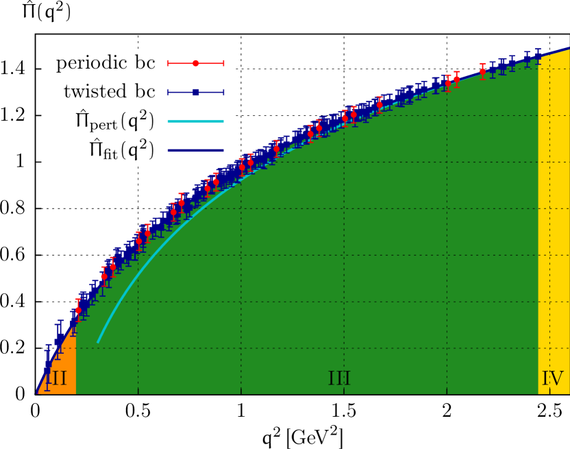
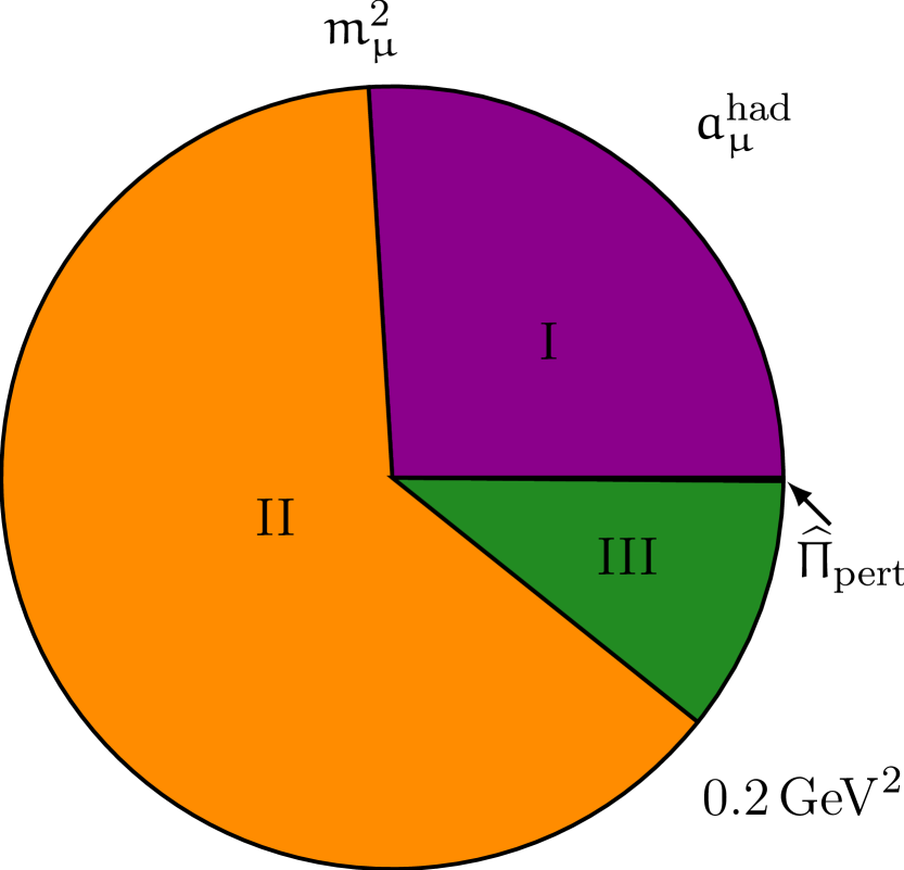
Figure 1: Left: The subtracted vacuum polarisation $\hat{\Pi}(q^{2})$ computed on the F6 ensemble ($\beta=\leavevmode\nobreak\ 5.3;$ $L=\leavevmode\nobreak\ 3.0\,\mathrm{fm};$ $m_{\pi}=\leavevmode\nobreak\ 323\,\mathrm{MeV}$) using twisted and periodic boundary conditions. The blue solid line shows the fit to the double vector ansatz c) matched to perturbation theory (light blue line). Right: The different contributions to $a_{\mu}^{\mathrm{HLO}}$ from the dispersion integral broken down to several momentum ranges, shown in both figures indicated by different colours.

The fits, except the vector dominance model fit, turn out to give consistent values within the statistical uncertainties, when the matching point of perturbation theory is chosen larger than $\approx 1\,\mathrm{GeV}$. In Figure 1 we show the subtracted vacuum polarisation together with the perturbation theory and fit c) (i.e. double vector). The effect of twisting is illustrated by showing periodic and twisted data in the same plot, which demonstrate a clear improvement on the momentum resolution of $\hat{\Pi}(q^{2})$. The remaining integration of Equation 4 is performed numerically. The right panel of Figure 1 shows the individual contributions to $a_{\mu}^{\mathrm{HLO}}$ separated into different momentum regions. Part I shows the area for $0$ to $m_{\mu}^{2}$, in which no data points occur. Nevertheless this small momentum range is constrained by the condition that $\hat{\Pi}(q^{2})\rightarrow 0$ for $q\rightarrow 0$ and the smooth behaviour of the fit curve. The second momentum range (II) displays the region in which twisted data points begin to contribute. In the third region (III) periodic and twisted data points give a perfect description of the momentum behaviour. The final section (IV) shows the contribution from perturbation theory, which turns out to be negligible. The overall statistical error, estimated via a bootstrap procedure, is dominated by regions I and II and ranges from $2\%$ to $7\%$ for the different ensembles.

4 Results

In Figure 2 we show the result for $a_{\mu}^{\mathrm{HLO}}$ computed for the ensembles listed in Table 1 as a function of $m_{\pi}^{2}$. We observe a clear curvature and steep rise for small pion masses. To obtain $a_{\mu}^{\mathrm{HLO}}$ at the physical point we need to perform a chiral extrapolation. In addition to a linear behaviour in $m_{\pi}^{2}$ we also include a logarithmic term, which is motivated by chiral perturbation theory

$$a_{\mu}^{\mathrm{HLO}}(m_{\pi}^{2})=a_{\mu}^{\mathrm{HLO}}+B\,m_{\pi}^{2}+C\,m_{\pi}^{2}\,\log(m_{\pi}^{2}).$$ (11)

We restrict the fit to the four most chiral $\beta=5.3$ data only to avoid mixing of cutoff effects and the chiral extrapolation.

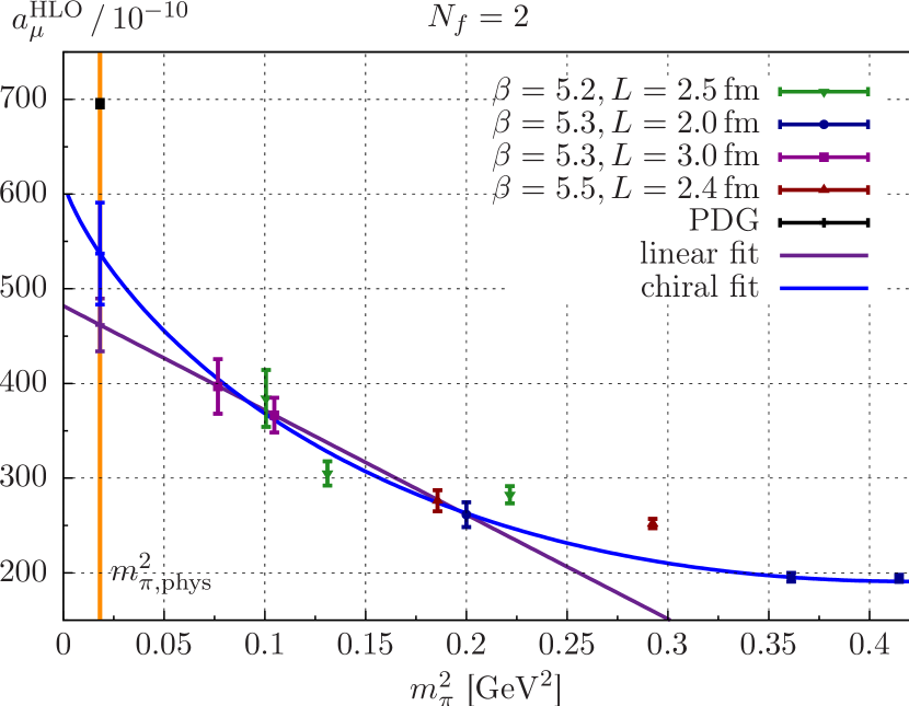
Figure 2: Left: The simulation results for the hadronic contribution to $a_{\mu}$ computed using two flavours, shown as function of $m_{\pi}^{2}$. The chiral extrapolation (blue curve) is performed using an ansatz motivated by chiral perturbation theory. Right: Corresponding results for $a_{\mu}^{\mathrm{HLO}}$ including a partially quenched strange quark.

We find that this extrapolation describes the whole set of data points quite well even those which not included in the fit. If we use this extrapolation, we obtain for $a_{\mu}^{\mathrm{HLO}}$ in the two-flavour case

$$a_{\mu}^{\mathrm{HLO}}(N_{f}=2)=537.1\,(53.8)_{\mathrm{stat}}\,(37.6)_{\mathrm{chiral}}\cdot 10^{-10}.$$ (12)

For the case of an additional quenched strange quark we end up with

$$a_{\mu}^{\mathrm{HLO}}(N_{f}=2+1_{Q})=612.4\,(49.9)_{\mathrm{stat}}\,(48.5)_{\mathrm{chiral}}\cdot 10^{-10}.$$ (13)

We repeat the analysis using a linear extrapolation for the $3$ most chiral $\beta=5.3$ data points to estimate the uncertainties from the chiral extrapolation by using half the difference of the central values.

Since finite size effects and cutoff effects rather depend on $q^{2}$, it is more instructive to study them using the subtracted vacuum polarisation $\hat{\Pi}(q^{2})$ than $a_{\mu}^{\mathrm{HLO}}$. The left panel of Figure 3 shows the quantity $\hat{\Pi}(q^{2})$ for two different ensembles which have roughly the same pion mass and volume. This allows us to look for cutoff effects, which turn out to be below $3\%$ in the momentum range $q^{2}<1\,\mathrm{GeV}^{2}$. The right panel of Figure 3 offers an insight to finite size effects and cutoff effects, showing two ensemble which differ in volume and lattice spacing. It turns out that these two effects are around $5\%$ and within our statistical precision.

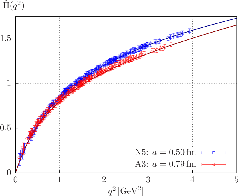
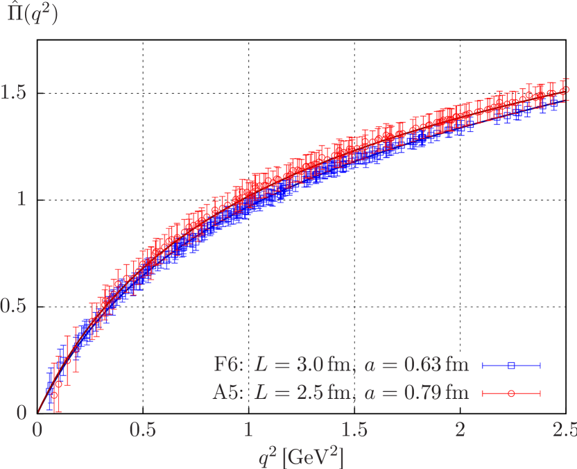
Figure 3: Left: A study of cutoff effects comparing the subtracted vacuum polarisation for two ensemble with roughly the same pion mass $m_{\pi}\approx 450\,\mathrm{MeV}$ and volume $L=2.5\,\mathrm{fm}$. Right: A comparison of $\hat{\Pi}(q^{2})$ for two ensemble with the same pion mass $m_{\pi}=320\,\mathrm{MeV}$.

5 Conclusions and Outlook

The determination of $a_{\mu}^{\mathrm{HLO}}$ using Lattice QCD is feasible, but still requires further improvements to make an impact on phenomenology. Partially twisted boundary conditions extend the accessible momentum range for the vacuum polarisation and thereby reduce the statistical and systematic uncertainties. At present the individual data points for $a_{\mu}^{\mathrm{HLO}}$ have statistical precision of $2\%$ to $7\%$. Summing up all individual uncertainties in quadrature we end up with an overall uncertainty of $\approx 12\%$ for the extrapolated value at the physical point. Our study of residual systematics indicate that finite size effects and cutoff effects change $a_{\mu}^{\mathrm{HLO}}$ slightly. The value will in any case decrease after the inclusion of the disconnected diagrams. Further details of our study will be published soon [21]. In the future we will study ensembles with smaller pion masses to improve the extrapolation to the physical point and reduce the systematics, such as finite size effects and cutoff effects. Once we are confident that we can control these effects to the required level of accuracy, we will include a dynamical strange and charm quarks into our calculations.

TEST

Acknowledgments: We thank Gilberto Colangelo, Achim Denig, Fred Jegerlehner, Harvey B. Meyer and Rainer Sommer for useful discussions. We are grateful to our colleagues within the CLS project for sharing gauge ensembles. Calculations of correlation functions were performed on the dedicated QCD platform "Wilson" at the Institute for Nuclear Physics, University of Mainz. This work was supported by DFG (SFB443) and the Research Center EMG funded by Forschungsinitiative Rheinland-Pfalz.

References

- [1] F. Jegerlehner and A. Nyffeler, The muon , Physics Reports 477 (2009) 1.
- [2] K. Jansen and R. Sommer, improvement of lattice QCD with two flavors of Wilson quarks , Nucl. Phys. B530 (1998) 185.
- [3] T. Blum, Lattice calculation of the lowest-order hadronic contribution to the muon anomalous magnetic moment, Phys. Rev. 91 (2003) 52001.
- [4] M. Göckeler, R. Horsley, W. Kürzinger, D. Pleiter, P.E.L. Rakow, and G. Schierholz, Vacuum polarization and hadronic contribution to muon from lattice QCD, Nucl. Phys. B688 (2004) 135.
- [5] X. Feng, M. Petschlies, K. Jansen, and D.B. Renner, Two-flavor QCD correction to lepton magnetic moments at leading-order in the electromagnetic coupling, arXiv:1103.4818 (2011).
- [6] D.B. Renner, these proceedings.
- [7] P. Boyle, L. Del Debbio, E. Kerrane, and J. Zanotti, Lattice determination of the hadronic contribution to the muon using dynamical domain wall fermions, arXiv:1107.1497 (2011).
- [8] E. Kerrane, these proceedings.
- [9] https://twiki.cern.ch/twiki/bin/view/CLS/WebIntro (2011).
- [10] G. von Hippel, these proceedings.
- [11] B. Knippschild, PhD Thesis (2011).
- [12] M. Della Morte and A. Jüttner, Quark disconnected diagrams in chiral perturbation theory, JHEP 11 (2010) 154.
- [13] E. De Rafael, Hadronic contributions to the muon and low-energy QCD, Phys. Lett. B322 (1994) 239.
- [14] C.T. Sachrajda and G. Villadoro, Twisted boundary conditions in lattice simulations, Phys. Lett. B609 (2005) 73.
- [15] M. Della Morte and A. Jüttner, New ideas for g-2 on the lattice, PoS LAT2009 (2009) 143.
- [16] K.G. Chetyrkin, J.H. Kühn, and M. Steinhauser, Three-loop polarization function and corrections to the production of heavy quarks, Nucl. Phys. B482 (1996) 213.
- [17] M. Della Morte, R. Frezzotti, J. Heitger, J. Rolf, R. Sommer, and U. Wolff, Computation of the strong coupling in QCD with two dynamical flavors, Nucl, Phys. B713 (2005) 378.
- [18] M. Della Morte, R. Hoffmann, F. Knechtli, J. Rolf, R. Sommer, I. Wetzorke, and U. Wolff, Non-perturbative quark mass renormalization in two-flavor QCD, Nucl. Phys. B729 (2005) 117.
- [19] M. Della Morte, R. Sommer, and S. Takeda, On cutoff effects in lattice QCD from short to long distances, Phys. Lett. B672 (2009) 407.
- [20] P. Fritzsch, J. Heitger, and N. Tantalo, Non-perturbative improvement of quark mass renormalization in two-flavour lattice QCD, JHEP, 08 (2010) 74.
- [21] M. Della Morte, B. Jäger, A. Jüttner and H. Wittig, in preparation.