Kelvin-Helmholtz instability in two-component Bose gases on a lattice

Abstract

We explore the stability of the interface between two phase-separated Bose gases in relative motion on a lattice. Gross-Pitaevskii-Bogoliubov theory and the Gutzwiller ansatz are employed to study the short- and long-time stability properties. The underlying lattice introduces effects of discreteness, broken spatial symmetry, and strong correlations, all three of which are seen to have considerable qualitative effects on the Kelvin-Helmholtz instability. Discreteness is found to stabilize low flow velocities, because of the finite energy associated with displacing the interface. Broken spatial symmetry introduces a dependence not only on the relative flow velocity, but on the absolute velocities. Strong correlations close to a Mott transition will stop the Kelvin-Helmholtz instability from affecting the bulk density and creating turbulence; instead, the instability will excite vortices with Mott-insulator filled cores.

I Introduction

The Kelvin-Helmholtz instability is a dynamical instability of the interface between two fluids that move relative to one another. This hydrodynamical instability can occur in very different settings, for example when the wind is blowing over the surface of the smooth ocean or in plasma flows in the Earth’s magnetic field Hasegawa2004a , or at the $AB$-phase boundary in superfluid ${}^{3}{\rm He}$ Blaauwgeers2002a ; Volovik2002a . The creation of degenerate mixtures of weakly interacting different bosonic gases Hall1998b ; Stenger1998a ; Modugno2001a enables studies of the Kelvin-Helmholtz instability in quantum systems which are more controllable as well as easier to measure in detail than more strongly interacting superfluids such as liquid ${}^{3}{\rm He}$. Takeuchi, Suzuki et al. takeuchi2010 ; suzuki2010 performed theoretical studies of the Kelvin-Helmholtz instability in a two-component condensate. Essentially, Ref. takeuchi2010 confirmed the expectation that Bose-Einstein condensed atomic gases provide an ideal setting to study the classic Kelvin-Helmholtz instability without viscosity complicating the picture. Ref.  suzuki2010 found a considerably altered instability dispersion relation in the case of a wide interface with large overlap between the two condensates; this was classified as a counter-superflow instability.

Putting a Bose gas in an optical lattice introduces several new features. Most dramatically, the gas exhibits a quantum phase transition between a superfluid and a Mott insulating state when the ratio between the tunneling and interaction energies passes a critical value jaksch1998 . In a binary condensate the phase diagram is richer, displaying different combinations of Mott insulator and superfluid in coexisting or phase separated configurations powell2009 ; iskin2010 . Moreover, even in the superfluid state where a significant portion of the atoms are Bose-Einstein condensed, the discreteness and the broken translational symmetry can have decisive effect on the motion of the bosons, as we shall see.

In this paper, we study the Kelvin-Helmholtz-type instabilities of a phase separated binary condensate on a lattice. In Sec. II, we present the equations that we work with. In Sec. III.1, we study a weakly segregated pair of condensates in order to explore the effects of broken translational symmetry on the interface dynamics. In Sec. III.2, we study instead a strongly segregated pair of condensates to see the effects of discreteness of the lattice. Sec. IV presents a heuristic derivation of a closed-form expression for the numerically obtained instabilities. In Sec. V, we study the system close to a Mott transition in order to explore the effects of strong correlations. Finally, in Sec. VI, we summarize and conclude.

II Theory of a two-component lattice Bose gas

The system is assumed to consist of two species of bosons at nearly zero temperature hopping on a square lattice, as can be realized with evaporatively cooled atoms in an optical lattice Hall1998b ; Stenger1998a ; Modugno2001a . If the lattice is deep enough, the tight-binding approximation is valid and the bosons can be assumed to occupy the lowest band only. For simplicity, we assume the two species to have equal masses, interaction constant and tunneling properties; this can be realized by choosing the two components to be two spin states of the same element. The many-body Hamiltonian governing this system is

$$\hat{H} = -\sum_{j=1}^{2}\sum_{<rr^{\prime}>}J_{j}\hat{a}^{\dagger}_{jr}\hat{a}_{jr^{\prime}}$$ (1)

$$+ \frac{1}{2}\sum_{j=1}^{2}U_{jj}\sum_{r}\hat{a}^{\dagger}_{jr}\hat{a}^{\dagger}_{jr}\hat{a}_{jr}\hat{a}_{jr}$$

$$+ U_{12}\sum_{r}\hat{a}^{\dagger}_{1r}\hat{a}_{1r}\hat{a}^{\dagger}_{2r}\hat{a}_{2r}-\sum_{j=1}^{2}\mu_{j}\sum_{r}\hat{a}^{\dagger}_{jr}\hat{a}_{jr}.$$

Here, $J_{j}$ are the tunneling matrix elements, $U_{jj}$ are the in-species interaction parameters and $U_{12}$ is the inter-species interaction parameter. $\mu_{j}$ is the chemical potential of species $j$. The summation index $j=1,2$ denotes the different species and the index $r$ runs over the lattice sites. We will be studying a two-dimensional square lattice in this paper, and we therefore pass to a vector notation, ${\bf r}=(x,z)$, where we let the dimensionless Cartesian coordinates $x$ and $z$ take on integer values.

For strong enough hopping and for high enough density, the lattice gases are almost entirely Bose-Einstein condensed and the problem can be treated using Gross-Pitaevskii and Bogoliubov analysis. This regime is suitable for identifying effects of the discreteness and broken translational invariance of the lattice, effects that do not depend on quantum fluctuations. In this regime, the lattice gas is accurately described using condensate wavefunctions $\Phi_{j}({\bf r},t)=\langle\hat{a}_{jr}\rangle$, whose dynamics follows from the discrete two-component Gross-Pitaevskii (GP) equation

$$i\frac{\partial\Phi_{1}({\bf r},t)}{\partial t} = -J_{1}\nabla^{2}\Phi_{1}({\bf r},t)+\left[U_{11}|\Phi_{1}|^{2}+U_{12}|\Phi_{2}|^{2}\right]\Phi_{1}({\bf r},t),$$

$$i\frac{\partial\Phi_{2}({\bf r},t)}{\partial t} = -J_{2}\nabla^{2}\Phi_{2}({\bf r},t)+\left[U_{22}|\Phi_{2}|^{2}+U_{12}|\Phi_{1}|^{2}\right]\Phi_{2}({\bf r},t),$$ (2)

where the discrete Laplacian is defined as

$$\nabla^{2}\Phi({\bf r})=\sum_{{\bf r}^{\prime}}\Phi({\bf r^{\prime}}),$$ (3)

and the sum over ${\bf r}^{\prime}$ runs over the nearest neighbors to the site ${\bf r}$.

II.1 Bogoliubov approach

In the Bogoliubov approximation one assumes for each component a stationary wavefunction with a small time-dependent perturbation,

$$\Phi_{1}({\bf r},t)=\left[\Psi_{1}(z,t)+\delta\Psi_{1}(x,z,t)\right]\exp(-i\mu t),$$

$$\Phi_{2}({\bf r},t)=\left[\Psi_{2}(z,t)+\delta\Psi_{2}(x,z,t)\right]\exp(-i\mu t).$$ (4)

The equation of motion to zeroth order is the time-independent 1D GP equation that is used to calculate the interface profile,

$$-J_{1}\frac{\partial^{2}\Psi_{1}(z)}{\partial z^{2}}+\left[U_{11}|\Psi_{1}(z)|^{2}+U_{12}|\Psi_{2}(z)|^{2}\right]\Psi_{1}(z) = \mu_{1}\Psi_{1}(z),$$

$$-J_{2}\frac{\partial^{2}\Psi_{2}(z)}{\partial z^{2}}+\left[U_{22}|\Psi_{2}(z)|^{2}+U_{12}|\Psi_{1}(z)|^{2}\right]\Psi_{2}(z) = \mu_{2}\Psi_{2}(z),$$ (5)

where we introduced notation analogous to Eq. (3),

$$\frac{\partial^{2}\Psi_{j}(z)}{\partial z^{2}}=\Psi_{j}(z+1)+\Psi_{j}(z-1).$$ (6)

Anticipating that the nonlinear term in the GP equation will couple positive- and negative-frequency modes, we define in a standard way

$$\delta\Psi_{i}({\bf r},t)=\left[u_{i}({\bf r},t)\exp(-i\omega t)+v_{i}^{*}({\bf r},t)\exp(i\omega t)\right]\exp(-i\mu t).$$

Ignoring the second order terms in the perturbations we get the Bogoliubov equations for the discrete double condensate system,

$${\hat{M}}{\bf v}=\omega{\hat{\eta}}{\bf v},$$ (7)

where

$${\hat{M}}=\left(\begin{array}[]{cccc}H_{1}&U\Psi_{1}^{2}&C&D\\ U\Psi_{1}^{*2}&H_{1}&D^{*}&C^{*}\\ C^{*}&D&H_{2}&U\Psi_{2}^{2}\\ D^{*}&C&U\Psi_{2}^{*2}&H_{2}\end{array}\right),$$ (8)

$${\hat{\eta}}=\left(\begin{array}[]{cccc}1&0&0&0\\ 0&-1&0&0\\ 0&0&1&0\\ 0&0&0&-1\end{array}\right),$$ (9)

and

$${\bf v}=\left(\begin{array}[]{c}u_{1}({\bf r})\\ v_{1}({\bf r})\\ u_{2}({\bf r})\\ v_{2}({\bf r})\end{array}\right).$$ (10)

The coefficients are defined through $C=U_{12}\Psi_{1}\Psi_{2}^{*}$, $D=U_{12}\Psi_{1}\Psi_{2}$, and $n_{i}=|\Psi_{i}|^{2}$,

$$H_{1}=-J_{1}\nabla^{2}+2U_{11}n_{1}+U_{12}n_{2}-\mu_{1},$$ (11)

and

$$H_{2}=-J_{2}\nabla^{2}+2U_{22}n_{2}+U_{12}n_{1}-\mu_{2}.$$ (12)

Let us repeat some common terminology and standard results fetter1972 : The norm of a Bogoliubov mode is defined as

$$||{\bf v}||=\sum_{r}{\bf v}^{{\dagger}}({\bf r})\hat{\eta}{\bf v}({\bf r}).$$ (13)

Unless the norm is zero, we are free to rescale the Bogoliubov vector so that its absolute value is unity. A mode with $||{\bf v}||=1$ is called a quasiparticle mode and a mode with $||{\bf v}||=-1$ is called a quasihole mode. If $\Psi$ is the ground state, then all the quasiparticle modes have positive eigenfrequencies and all quasihole modes have negative eigenfrequencies; otherwise, no such rule applies. A mode with complex eigenfrequency has zero norm. Such modes will grow exponentially in time and thus they signal a dynamical instability. We will therefore be interested in the imaginary parts of the Bogoliubov eigenfrequencies in this article.

The symmetries of the problem give rise to degeneracies in the Bogoliubov spectrum. First, the well-known quasiparticle-quasihole symmetry of the Bogoliubov equations fetter1972 carries over to the two-component case: Each real eigenvalue $\omega$ with an eigenvector ${\bf v}=\left(u_{1}({\bf r}),v_{1}({\bf r}),u_{2}({\bf r}),v_{2}({\bf r})\right)^{T}$ has a corresponding solution with an eigenvalue $-\omega$ and an eigenvector

$${\bf v}=-\left(v_{1}({\bf r})^{*},u_{1}({\bf r})^{*},v_{2}({\bf r})^{*},u_{2}({\bf r})^{*}\right)^{T}.$$ (14)

In addition, imaginary eigenvalues appear in pairs of $\omega$ and $\omega^{*}$. Since we will be mostly interested in a symmetric interface where $\Psi_{1}({\bf r})=\Psi_{2}(-{\bf r})$, we have an additional degenerate solution

$$\left(u_{2}(-{\bf r}),v_{2}(-{\bf r}),u_{1}(-{\bf r}),v_{1}(-{\bf r})\right)^{T},$$ (15)

with eigenvalue $\omega$. Combining Eqs. (14-15) to obtain

$$\left(v_{2}^{*}(-{\bf r}),u_{2}^{*}(-{\bf r}),v_{1}^{*}(-{\bf r}),u_{1}^{*}(-{\bf r})\right)^{T},$$ (16)

with eigenvalue $-\omega$. The latter two symmetries hold strictly only when equal and opposite currents are induced in the two components, as we will discuss further below.

II.1.1 One moving condensate

The discrete system is not translationally invariant, and we can therefore not use the relative velocity of the condensates as a unique parameter; also the absolute individual currents are physically relevant. In particular, we will study two different cases: the case where only one of the condensates carries a current, and that where the condensates support equal but counter-flowing currents.

We first assume that component $2$ is moving along the $x$ direction and that all other position dependence of the stationary solutions is along $z$. Furthermore, the stationary wavefunctions can be taken as real. This means $\Psi_{1}({\bf r})=\Psi_{1}(z)$ and $\Psi_{2}({\bf r})=\Psi_{2}(z)\exp(ikx)$, with $-\pi<k\leq\pi$. We then have $C=U_{12}\Psi_{1}(z)\Psi_{2}(z)\exp(-ikx)$, $D=U_{12}\Psi_{1}(z)\Psi_{2}(z)\exp(ikx)$, and

$$H_{2}=-J_{2}\nabla^{2}+2U_{22}n_{2}+U_{12}n_{1}-\mu_{2}-2J_{2}(1-\cos k),$$ (17)

where $\mu$ is the chemical potential of the second component in the absence of a current; the term $2J(1-\cos k)$ due to the current is made explicit for convenience. The excitations can be expanded as plane waves along the $x$ direction. Dependency on the $x$ coordinate is eliminated with the choice

$$u_{1}({\bf r})=u_{1}(z)\exp(ik_{e}x-ikx/2),$$

$$v_{1}({\bf r})=v_{1}(z)\exp(ik_{e}x-ikx/2),$$

$$u_{2}({\bf r})=u_{2}(z)\exp(ik_{e}x+ikx/2),$$

$$v_{2}({\bf r})=v_{2}(z)\exp(ik_{e}x-3ikx/2).$$ (18)

The Bogoliubov equations now reduce to a 1D problem, and the Bogoliubov matrix takes the form

$${\hat{M}}_{\rm 1D}=\left(\begin{array}[]{cccc}H_{1u}&U\Psi_{1}^{2}&C&D\\ U\Psi_{1}^{*2}&H_{1v}&D^{*}&C^{*}\\ C^{*}&D&H_{2u}&U\Psi_{2}^{2}\\ D^{*}&C&U\Psi_{2}^{*2}&H_{2v}\end{array}\right),$$ (19)

where the diagonal elements are

$$H_{1u}=H_{1v}=-J_{1}\frac{\partial^{2}}{\partial z^{2}}+2J_{1}\left[1-\cos(k_{e}-k/2)\right]+2U_{11}n_{1}+U_{12}n_{2}-\mu_{1},$$

$$H_{2,u_{2}}=-J_{2}\frac{\partial^{2}}{\partial z^{2}}-2J_{2}(1-\cos k)+2J_{2}\left[1-\cos(k_{e}+k/2)\right]+2U_{22}n_{2}+U_{12}n_{1}-\mu_{2},$$

$$H_{2,v_{2}}=-J_{2}\frac{\partial^{2}}{\partial z^{2}}+-2J_{2}(1-\cos k)+2J_{2}\left[1-\cos(k_{e}-3k/2)\right)]+2U_{22}n_{2}+U_{12}n_{1}-\mu_{2}.$$ (20)

II.1.2 Counter-directed currents

In the case of equal and opposite currents in the respective components, we write $\Psi_{1}(x,z)=\Psi_{1}(z)e^{ikx/2}$ and $\Psi_{2}(x,z)=\Psi_{2}(z)e^{-ikx/2}$. The excitations can now be written

$$u_{1}({\bf r}) = u_{1}(z)e^{ik_{e}x+ikx/2},$$

$$v_{1}({\bf r}) = v_{1}(z)e^{ik_{e}x-ikx/2},$$

$$u_{2}({\bf r}) = u_{2}(z)e^{ik_{e}x-ikx/2},$$

$$v_{2}({\bf r}) = v_{2}(z)e^{ik_{e}x+ikx/2}.$$ (21)

We find that the off-diagonal terms of the matrix $\hat{M}_{\rm 1D}$ are the same as before, but to the diagonal we get

$$H_{1,u_{1}}=-J_{1}\frac{\partial^{2}}{\partial z^{2}}-2J_{1}(1-\cos k/2)+2J_{1}\left[1-\cos(k_{e}+k/2)\right]+2U_{11}n_{1}+U_{12}n_{2}-\mu_{1},$$

$$H_{1,v_{1}}=-J_{1}\frac{\partial^{2}}{\partial z^{2}}-2J_{1}(1-\cos k/2)+2J_{1}\left[1-\cos(k_{e}-k/2)\right]+2U_{11}n_{1}+U_{12}n_{2}-\mu_{1},$$

$$H_{2,u_{2}}=-J_{2}\frac{\partial^{2}}{\partial z^{2}}-2J_{2}(1-\cos k/2)+2J_{2}\left[1-\cos(k_{e}-k/2)\right]+2U_{22}n_{2}+U_{12}n_{1}-\mu_{2},$$

$$H_{2,v_{2}}=-J_{2}\frac{\partial^{2}}{\partial z^{2}}-2J_{2}(1-\cos k/2)+2J_{2}\left[1-\cos(k_{e}+k/2)\right]+2U_{22}n_{2}+U_{12}n_{1}-\mu_{2}.$$ (22)

Expressed in the reduced 1D Bogoliubov amplitudes $u_{j}(z),v_{j}(z)$, the symmetries (14-16) acquire new forms, since the effective Hamiltonians appearing in the diagonal of the Bogoliubov eigenvalue problem are different. The symmetry of greatest interest to us is that for a given $k$ and $k_{e}$, each real eigenvalue $\omega$ with a reduced eigenvector $\left(u_{1}(z),v_{1}(z),u_{2}(z),v_{2}(z)\right)^{T}$ now has a corresponding hole mode with eigenvalue $-\omega$ and reduced eigenvector

$$\left(v_{2}(-z),u_{2}(-z),v_{1}(-z),u_{1}(-z)\right)^{T}.$$ (23)

III Kelvin-Helmholtz instability in a discrete system

After assuming that the two condensates have equal chemical potentials $\mu_{1}=\mu_{2}=\mu$, tunneling $J_{1}=J_{2}=J$, and interaction strengths $U_{11}=U_{22}=U$, the system can be characterized by three parameters. These are chosen to be the ratios $J/U$ and $U_{12}/U$, and the number density per site far from the interface, $\bar{n}$. The chemical potential $\mu$ can then be calculated for given $J$, $U_{12}$, and $\bar{n}$. In addition, the problem is characterized by the wave vectors for the flow in each of the components, $(k_{1},k_{2})$. In Sec. II, we derived the detailed form of the Bogoliubov equations for one moving condensate, $(k_{1},k_{2})=(0,-k)$; and opposite currents, $(k_{1},k_{2})=(k/2,-k/2)$.

III.1 Weak coupling and broken translational symmetry

We first consider the case $J/U=1$, $U_{12}/U=1.1$, $\bar{n}=1$. Figure 1 shows the stability properties of the system in the case of one moving condensate, $(k_{1},k_{2})=(0,-k)$.

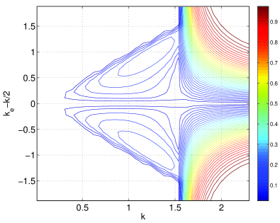
Figure 1: (Color online) Growth rate of the dynamically most unstable mode (i.e. the imaginary part of the mode with the largest imaginary frequency) as a function of flow wavevector $k$ and and mode wavevector $k_{e}$ (note that a shift $k_{e}-k/2$ has been applied to the y-axis to make the symmetry around $k_{e}=k/2$ more transparent). Here, one component is in motion with wavevector $k$ and the other is stationary. The lattice has $256$ sites, the parameter values are $J/U=1$, $U_{12}/U=1.1$, and the asymptotic density is $\bar{n}=1$.

The figure plots the largest imaginary excitation frequency as a function of flow wavevector $k$ and excitation wavevector $k_{e}$; thus, a vertical cross-section in the figure at a fixed $k$ gives the imaginary part of the spectrum for a given current. The lattice is of finite size, $256$ sites, in the numerics (in fact, real-life lattices may be of similar dimensions) and this influences the numerical value of the imaginary part somewhat. The effect is such that the imaginary part becomes larger as the lattice size is reduced to $128$. The physics at low wavevector $k$ is clearly recognized from the case of a pair of classical fluids or a homogeneous two-component BEC takeuchi2010 ; suzuki2010 ; chandrasekhar1961book ; gerwin1968RMP . For a given $k$, not too large, a range of excitations with wavevectors $0<|k_{e}-k/2|\lesssim k$ become unstable. The amplitudes of the unstable modes are localized at the interface, indicating that these are indeed interface modes.

We compare to the case of a continuous, i.e., non-lattice system. In Ref. suzuki2010 , it was observed that in the case of a narrow interface, the binary condensate displays the classical dispersion relation chandrasekhar1961book

$$\omega=\sqrt{\frac{\alpha}{2\rho}k_{e}^{3}-v^{2}k^{2}}\quad{\rm(classically),}$$ (24)

where $v$ is the velocity of the unperturbed flow and $\alpha$ is the surface tension. However, if the interface is wider, the upper stability line lies close to the line $|k_{e}-k/2|=k$; this was in Ref. suzuki2010 termed the counter-superflow instability. Apparently, Fig. 1 is in this latter regime, and the discreteness is not seen to cause considerable deviations from the linear stability line.

We note a few curious features in Fig. 1. For very small $k$, the instability seems to be absent; this will be discussed further in Sec. III.2. For wavevectors exceeding a critical value, $k>k_{c}=\pi/2$, it is seen in Fig. 1 that all excitation wavevectors become unstable. This is no longer an interface mode, but an instability known to occur also in single-component discrete BECs desarlo2005 . The physics behind the instability is that the single-particle dispersion relation, $\epsilon_{k}=J(1-\cos k)$, has an inflection point at $k_{c}$, and thus the effective mass goes from positive, to diverging, to negative. This is well understood and studied in single-component BECs and we will not dwell on it further, but only conclude that the interesting range of $k$ values for the case $(k_{1},k_{2})=(0,-k)$ ranges between $-\pi/2$ and $\pi/2$.

To illustrate the long time behavior of Kelvin-Helmholtz instability, we simulate the time development of the discrete GP equation. A series of snapshots are shown in Fig. 2 for the case $k=5\pi/64\approx 0.245$.

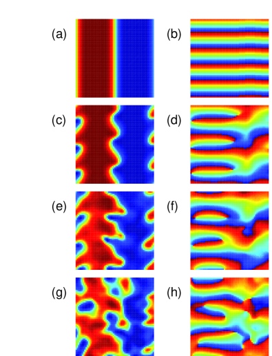
Figure 2: (Color online) Time development of the instability for the case $k=5\pi/64$, and remaining parameter values as in Fig. 1. Panels (a),(c),(e),(g) show the density of the 1 component, where red indicates high density and blue is zero density; panels (b), (d), (f), (h) show the corresponding phase. Snapshots are taken at times $t=44$ for (a)-(b); $t=176$ for (c)-(d); $t=265$ for (e)-(f); and $t=400$ for (g)-(h).

The time development is simulated using a split-step Fourier technique, with a grid of size 64$\times$64 sites and periodic boundary conditions along both directions. For the chosen wavevector $k=5\pi/64$, a surface wave with a dominant wavevector $k_{e}=3\pi/64$ can be seen to grow exponentially until the nonlinear stage is reached, where the condensates break up into smaller fragments.

For the case of counterflow, $(k/2,-k/2)$, the result for the imaginary parts of the modes is shown in Fig. 3.

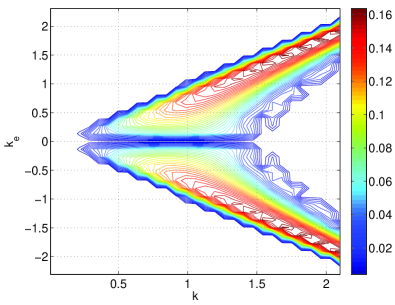
Figure 3: (Color online) Largest imaginary part of the excitation frequency as in Fig. 1, but with counter-flowing condensates having wavevectors $(k/2,-k/2)$. The lattice has $256$ sites, parameter values are $J/U=1$, $U_{12}/U=1.1$, and the asymptotic density is $\bar{n}=1$.

By definition of $k$, the critical relative wavevector for negative effective mass is in this case $k_{c}=\pi$. For large enough $k$, it is seen that the modes with small wavevectors $k_{e}$ are actually stabilized. We thus define a second critical wavenumber for the flow, $k_{s}$, above which long-wavelength excitations are stabilized. The corresponding flow velocity is denoted $v_{s}$. From Figure 3, we read off $k_{s}\approx 1.5$ (the closeness to $\pi/2$ is suggestive but, in fact, a coincidence). This is a counterpart to the classically known stabilization of long wavelengths when the flow velocity exceeds $\sqrt{8}$ times the sound speed $c$ gerwin1968RMP ,

$$v_{s}=\sqrt{8}c\quad{\rm(classically).}$$ (25)

However, in the discrete case, there seems to be no simple relationship between the onset of long-wavelength stability and sound speed. In this particular case, the flow velocity in each component is $v_{s}=2J\sin(k_{s}/2)\approx 1.4U$ in dimensionless units, whereas the sound speed is $c=\sqrt{JU\bar{n}}=U$, but further numerical experimentation shows only a weak dependence of $v_{s}$ on $c$; this puzzle will be resolved in Sec. IV.

Since the system lacks Galilean invariance, the spectrum for a given flow wavevector $k$ is not invariant under a transformation $(k_{1},k_{1})\to(k_{1}-q,k_{2}+q)$. We plot as an example in Fig. 4 the imaginary frequency for the same parameters as above, for two choices of $k$, comparing the cases $(k,0)$ and $(k/2,-k/2)$.

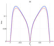
Figure 4: (Color online) Comparison of the largest imaginary part of the excitation frequency as a function of the excitation wavenumber $k_{e}$, in the cases of one flowing component, $(k,0)$ (dashed red), and counterflow, $(k/2,-k/2)$ (solid blue). Parameter values are as in Fig. 1, but the wavevector is fixed at $k=1.3$ in (a), and $k=1.0$ in (b). For the case of one flowing component, the $k_{e}$ axis is shifted by $k_{e}\to k_{e}-k/2$. The lattice has $256$ sites, parameter values are $J/U=1$, $U_{12}/U=1.1$, and the asymptotic density is $\bar{n}=1$.

It is seen that the curves are similar, but the symmetric case $(k/2,-k/2)$ is more unstable, in the sense that it has a higher maximum imaginary frequency. Further numerical experimentation (not shown here) indicates that this observation holds quite generally.

III.2 Narrow interface physics: Effects of discreteness

Figure 5 shows the stability spectrum of a system at a higher density, $\bar{n}=4$, and a stronger repulsion between the components, $U_{12}=1.5U$.

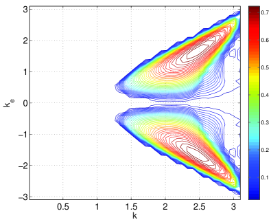
Figure 5: (Color online) Growth rate of the dynamically most unstable mode (i.e. the imaginary part of the mode with the largest imaginary frequency) as a function of flow wavevector $k$ and and mode wavevector $k_{e}$. Here, both components are in motion with counter-directed wavevectors $(k/2,-k/2)$. The parameters are $J/U=1$, $U_{12}/U=1.5$, and the asymptotic density is $\bar{n}=4$.

The combined effect of increased density, which means larger interaction energy, and increased inter-species repulsion, implies a narrower interface ao1998 . Already in the case $\bar{n}=1,U_{12}=1.1U$, we saw that low flow velocities appeared to be stable, and here the effect is more pronounced. This feature of the instability is not seen in simulations of homogeneous BECs takeuchi2010 ; suzuki2010 , nor in classical fluids, in the absence of external forces chandrasekhar1961book . We attribute this to the discrete density profile at the interface, as will be detailed below.

In the figure, we note also that there is a stable region for large flow wavevectors $k>k_{s}$, just as in the case $\bar{n}=1$, but now $k_{s}\approx 2.8$. We will return to this in Sec. IV. Finally, we observe that the upper instability line at large $k$ values is still approximately linear with unit slope, indicating that we are in the counter-superflow regime despite the narrower interface.

We now turn to the stability of slow flow wavevectors $k$. First recall how a dynamical instability in the Bogoliubov equations result from a collision between a quasiparticle mode and a quasihole mode lundh2006b . Starting from a reference point in phase space – here, take $k=0$ – we consider a quasiparticle mode ${\bf v}_{a}$ and a quasihole mode ${\bf v}_{b}$ with real, nearly degenerate eigenfrequencies $\omega_{0a}$ and $\omega_{0b}$. We then slightly increase a control parameter – in this case, $k$ – and thus transform the Bogoliubov matrix $M\to M^{\prime}=M+\delta M$. Writing ${\bf v}=a{\bf v}_{a}+b{\bf v}_{b}$ and solving the Bogoliubov equations for the new eigenfrequencies $\omega$, we find in the general case

$$\omega=\frac{\omega_{0a}+\omega_{0b}+\delta\omega_{a}+\delta\omega_{b}}{2}\pm\sqrt{\left(\frac{\omega_{0a}-\omega_{0b}+\delta\omega_{a}-\delta\omega_{b}}{2}\right)^{2}-|X|^{2}},$$ (26)

where $\delta\omega_{a}={\bf v}_{a}^{{\dagger}}\delta M{\bf v}_{a}$, $\delta\omega_{b}=-{\bf v}_{b}^{{\dagger}}\delta M{\bf v}_{b}$, and $X={\bf v}_{a}^{{\dagger}}\delta M{\bf v}_{b}$. In other words, when the two modes become degenerate, the cross-term makes them unstable.

In the present case, we consider two modes related by the symmetry of Eq. (23); thus, we have $\omega_{0a}+\delta\omega_{a}=-\omega_{0b}-\delta\omega_{b}$, and

$$\omega=\pm\sqrt{\left(\omega_{0a}+\delta\omega_{a}\right)^{2}-|X|^{2}}.$$ (27)

In a homogeneous, i.e., non-discrete system, the lowest-lying surface mode corresponds to a uniform translation of the boundary and is thus a Goldstone mode; at $k=k_{e}=0$ it has zero energy, i.e., $\omega_{0a}=0$ in the limit $k_{e}=0$. With increasing $k_{e}$, its energy increases from zero. A finite $k$ results in a shift in the Bogoliubov matrix $\delta M$ as discussed above and the Kelvin-Helmholtz instability comes about because $|X|$ is always greater than $\delta\omega_{a}$ in these systems. The onset of instability therefore tends towards $k=0$ as $k_{e}$ tends to zero.

In a discrete system, however, translational symmetry is lost and there is no Goldstone mode: A small shift of the boundary profile costs a finite amount of energy. This translates into $\omega_{0a}=\epsilon>0$ at $k_{e}=0$, which in turn creates a threshold value of $k$ for the onset of instability. For stronger interactions or higher densities, the interface is thinner, and the effects of discreteness are more pronounced. This explains the increased threshold value for higher density.

Figure 6 displays some of the lowest-lying Bogoliubov eigenvalues for a fixed $k_{e}=0.3$, as functions of $k$, at $\bar{n}=4$.

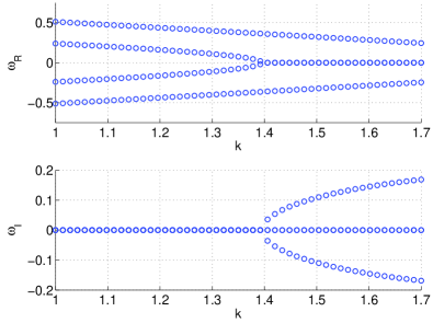
Figure 6: Few Bogoliubov eigenvalues for a fixed excitation wavevector $k_{e}=0.3$, as functions of the flow wavevector $k$. Parameters are as in Fig. 5. Upper panel: Real parts, lower panel: Imaginary parts.

It is clearly seen how instabilities result from a merging of two eigenstates with equal but opposite energies, thus related by the symmetry in Eq. (23). For large $k$ similar instabilities happen for many other modes and here, for clarity, we plot just the appearance of the first instability. The modes responsible for the dominant instability start out at a small but finite energy for $k=0$; this energy does not tend to zero as $k_{e}\to 0$ (although the latter fact cannot be inferred from the figure). The mode functions $u_{i},v_{i}$ are plotted in Fig. 7.

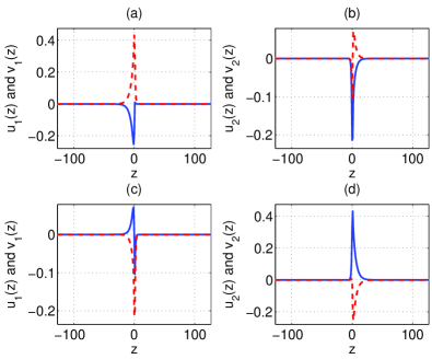
Figure 7: Bogoliubov eigenstates for the lowest-lying surface modes, functions $u_{j}(z)$ (blue solid lines) and $v_{j}(z)$ (red dashed) at $k_{e}=0.3$ and $k=1.25$, which is below the instability threshold. Upper panels: Quasiparticle mode; Lower panels: Quasihole mode. Left panels: mode functions $u_{1}(z),v_{1}(z)$ associated with component 1, and right panels: mode functions $u_{2}(z),v_{2}(z)$. The lattice has $256$ sites, parameter values are $J/U=1$, $U_{12}/U=1.5$, and the asymptotic density is $\bar{n}=4$.

These are the lowest-lying surface modes corresponding to translation of the surface; notice how the symmetry (23) is manifest in the plots.

IV Towards an analytical description

In order to obtain a feeling for the mathematics and physics behind the Kelvin-Helmholtz instability, we show here a heuristic derivation of an approximate analytical formula for the excitation frequencies. In effect, we replace the spatially dependent coefficients in Eq. (19) by c-numbers. This can be justified by expanding the solution $\mathbf{v}$ in a suitable basis nilsen2008 . It can also be effected by simply assuming a local-density approximation at the center of the interface. We discuss the more symmetric case with counter-directed currents, $(k_{1},k_{2})=(k/2,-k/2)$, since it allows for solutions on closed form. The matrix is approximated as

$${\hat{M}}=\left(\begin{array}[]{cccc}\epsilon+\Delta_{+}+g&g&C&C\\ g&\epsilon+\Delta_{-}+g&C&C\\ C&C&\epsilon+\Delta_{-}+g&g\\ C&C&g&\epsilon+\Delta_{+}+g\end{array}\right),$$

where $g$ is proportional to the in-species interaction energy, and $C$ is a measure of the inter-species repulsion. $\epsilon$ is a self-energy associated with bending in the $z$ direction of the respective mode function, which is to be identified with the finite energy $\omega_{0a}$ of the almost-Goldstone modes dicussed above. Finally, $\Delta_{\pm}$ are the relative kinetic energies. In the discrete lattice case,

$$\Delta_{\pm}=-2J(1-\cos k/2)+2J\left[1-\cos(k_{e}\pm k/2)\right],$$ (28)

and in the continuous case without a lattice,

$$\Delta_{\pm}=\frac{\hbar^{2}}{2m}(k_{e}^{2}\pm k_{e}k).$$ (29)

The continuous case is simplest: Inserting the dispersion, putting $\hbar=m=1$ for convenience, we obtain the eigenfrequencies

$$\omega^{2}=(2g+\frac{1}{2}k_{e}^{2}+\epsilon)(\epsilon+\frac{1}{2}k_{e}^{2})+\frac{1}{4}k_{e}^{2}k^{2}\pm 2\sqrt{\epsilon+\frac{1}{2}k_{e}^{2}}\sqrt{(2g+\epsilon+\frac{1}{2}k_{e}^{2})\frac{1}{4}k_{e}^{2}k^{2}+C^{2}(\epsilon+\frac{1}{2}k_{e}^{2})}.$$ (30)

This equation is of the same form as that in Ref. suzuki2010 , describing the counter-superflow instability. Clearly, the case with a minus sign lets $\omega^{2}$ become negative for certain parameter values, and thus describes the unstable modes. The discrete case yields somewhat clumsier expressions, but can be solved; we discuss the differences below.

The choice of parameters can be done with the benefit of hindsight; however, assuming a local-density approximation in the midpoint of the interface, where in the limit of a broad interface the densities $n_{1}$ and $n_{2}$ are half their bulk values, we readily obtain $g=U{\bar{n}}/2=\mu/2$, and $C=U_{12}\bar{n}/2=(U_{12}/U)g$. The self-energy $\epsilon$ is smaller than the other energies, and so is $C-g$, so we first put $\epsilon=0$ and $C=g$ in Eq. (30) and find the points where $\omega^{2}$ turns negative; these are the boundaries for instability. We obtain the solutions

$$k_{e}=0,$$

$$k=k_{e},$$

$$k^{2}-k_{e}^{2}-4\mu=0.$$ (31)

Linearizing around the first instability, we obtain

$$\omega^{2}=\frac{1}{2}k_{e}^{2}\left(\epsilon-\frac{1}{2}k^{2}\right)+{\mathcal{O}}(k_{e}^{4}),$$ (32)

which is the well-known linearly increasing imaginary frequency, existing for $k^{2}<4\mu$. The modes are stabilized again when $k_{e}>k$. The upper stability limit lies at $k_{e}=k$ as observed in Ref. suzuki2010 . However, when $k^{2}>4\mu$, small wavevectors $k_{e}$ are stabilized. This is similar to the well known classical stabilization at relative flow velocities exceeding $\sqrt{8}$ times the sound velocity, as we discussed in Sec. III.1 gerwin1968RMP . However, even in the continuous case, the prefactor does not match with the classical result (nor with Ref. suzuki2010 ); we simply attribute this to the quite different kind of dispersion relation.

A small but finite $\epsilon$ will introduce small corrections to the above. In order to salvage the linear dispersion at small excitation wavevectors $k_{e}$ – which is observed to be the case numerically – we must put $C=g+\epsilon/2$. With a finite $\epsilon$, slow flow velocities are stabilized. This happens only in the discrete case, but in order to bring out the qualitative features while displaying reasonably compact formulas, we show here the bastardized expression resulting from using a continuous-case dispersion relation together with a finite self-energy. Expanding the eigenfrequency in powers of $k$ and $k_{e}$, one obtains

$$\omega^{2}=\frac{1}{2}k_{e}^{2}(\frac{1}{2}k_{e}^{2}+\epsilon)-\frac{1}{4}k^{2}k_{e}^{2}+{\mathcal{O}}(k^{6},k_{e}^{6},k^{2}k_{e}^{4},k^{4}k_{e}^{2}),$$ (33)

which is positive for $k^{2}<q^{2}+2\epsilon$. Thus, slow flow velocities are seen to be absolutely stable. Classically, this only happens in the presence of gravity or an equivalent asymmetric force chandrasekhar1961book ; takeuchi2010 , but in the discrete system, there is stabilization even in the absence of forces.

The discrete-case dispersion relation leads to more complicated algebra, but all the qualitative conclusions remain the same. When $\epsilon=0$ and $g=C$, the frequency is again zero for $k_{e}=0$ and $k_{e}=k$; a finite $\epsilon$ stabilizes small $k$. The most important modification is that of the sound-speed limit, where we now obtain stability at small $k_{e}$ if $k>k_{s}$, with $k_{s}$ given by

$$2J\cos(\frac{k_{s}}{2})=-\mu/2+\sqrt{\mu^{2}/4+4J^{2}},$$ (34)

whose solution is always real. The continuous-case expression is recovered when $\mu/J$ is small; then the flow velocity is $v_{s}=2J\sin k_{s}\approx\sqrt{4\mu}$, similar to the continuous case.

Furthermore, for $k>\pi/2$, the spectrum changes character completely and a wide range of excitation wavevectors $k_{e}$ become unstable; this is again a manifestation of the bulk instability associated with negative effective mass of Ref. desarlo2005 .

Thus, a heuristic constant-amplitude calculation has managed to bring out all the features present in the numerical results. The familiar linear increase of imaginary frequency at small $k_{e}$ for a given flow wavevector $k$; the stabilization at excitation wavevectors $k_{e}$ exceeding $k$; the absolute stabilization of slow relative velocities; the stabilization of small $k_{e}$ for $k$ above a cutoff depending on the sound velocity; and even the bulk instability when the effective mass becomes negative, could all be described.

V Strongly correlated regime

The discussion so far has been limited to the case of two Bose gases in the Bose-Einstein condensed state. This is the state of the system when the ratio $J/U$ is not very small and when the density is not very small. In the general case, one must account for quantum fluctuations whose most striking effect is to drive a quantum phase transition between the superfluid and Mott insulating phases jaksch1998 . In addition, quantum fluctuations are seen to shift the transition line between mixed and phase-segregated phases, as we shall see below.

The many-body Hamiltonian (1) has been seen to display a rich phase diagram powell2009 ; iskin2010 . In Figure 8, we display the portion of greatest interest for our purposes.

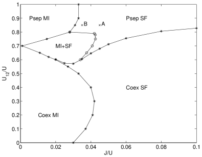
Figure 8: Phase diagram for a mixture of two identical Bose gases, calculated in the Gutzwiller approximation. The chemical potential is taken to be $\mu=0.7U$. The points A and B mark the parameters for which the two simulations described in the text are done.

The phase diagram is calculated in the Gutzwiller approximation, which is explained below. The general picture is that for weak enough hopping $J$, except in degenerate cases, both gases are in the Mott insulating state (marked MI in Fig. (8)) with suppressed on-site number fluctuations and zero superfluid density; conversely, for large enough $J$ the bosons are always superfluid (SF). If the inter-component interaction $U_{12}$ is large enough compared with the chemical potential $\mu$, then the two components are phase separated (marked Psep), either Mott insulating or superfluid; and if $U_{12}$ is small enough or $\mu$ big enough, the two components coexist (marked Coex). There exists one further phase close to the line $U_{12}=\mu$ at weak hopping, where one component is Mott insulating and the other one is superfluid with a lower density (marked SF+MI in the phase diagram). Finally, note that for a pair of Bose-Einstein condensed gases, the transition between phase separated and coexisting phases takes place at $U_{12}=U$. In contrast, in the limit of weak $J$, phase separation takes place at $U_{12}=\mu$.

The Gutzwiller approximation is based on a mean-field ansatz for the many-body state,

$$|\psi_{G}(t)\rangle=\prod_{r}\prod_{j=1}^{2}|\phi_{r,j}(t)\rangle.$$ (35)

This ansatz amounts to treating both the hopping between sites and the inter-species interaction in a mean-field fashion. This can be done since on-site entanglement between the two species is not expected to be important. For computations, it is convenient to expand the on-site states in a local Fock basis with an upper cutoff $n_{\rm max}$,

$$|\phi_{r,j}(t)\rangle=\sum_{n=0}^{n_{\rm max}}C_{r,j,n}(t)|n\rangle_{r,j}.$$ (36)

In the Gutzwiller approximation, the local total density $n$ and condensate wave function $z$ for each of the components is readily computed. We characterize the system by studying the behavior of local density $n_{j}$, the local condensate density $n_{cj}=|\Phi_{j}|^{2}$, and phase $\varphi_{j}={\rm arg}\Phi_{j}$. In order to calculate the ground state, the Hamiltonian (1) is minimized with respect to the complex coefficients $C_{r,j,n}$. To simulate dynamics, we propagate the coupled equations of motion zakrzewski2005 ; lundh2011

$$i\frac{\partial C_{r,j,n}}{\partial t}=\frac{\delta}{\delta C_{r,j,n}^{*}}\langle\psi_{G}(t)|H|\psi_{G}(t)\rangle.$$ (37)

For the present simulation of Kelvin-Helmholtz physics, the initial condition was constructed by calculating the phase separated ground state, then imprinting counter-directed currents on the two components, and finally adding a small amount of random noise onto each of the complex coefficients $C_{r,j,n}$.

We simulate interface dynamics in the “Psep SF” phase. In the Mott insulating phase, dynamics is quite trivially absent. In the “SF+MI” phase, there is also no interface dynamics: Since the Mott-superfluid phase transition is second order, there is no surface tension and hence no capillary waves are expected to form between superfluid and Mott insulating regions. Phenomena connected to melting of Mott insulators are conceivable at high enough energies (cf. lundh2011 ; krutitsky2011 ), but we will not pursue this here.

The first simulation is done at the point marked A in the phase diagram of Fig 8: $J=0.045U,U_{12}=0.85U$, and $\mu=0.7U$. Here, we have two phase separated superfluids, and as seen in Fig. 9, the Bose-Einstein condensed part of the fluid is less than half the total density.

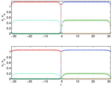
Figure 9: (Color online) Cross sections of the density profile of two phase segregated Bose gases at points A (upper panel) and B (lower panel) in the phase diagram, respectively. Squares denote the density for component 1 $n_{1}$; crosses denote $n_{c1}$; asterisks $n_{2}$, and circles $n_{c2}$. Lines are to guide the eye.

Also the superfluid density is expected to be small close to the Mott transition rey2003 . Figure 10 shows the dynamics of a system with symmetrically imprinted wavevectors $(k/2,-k/2)$, where $k=7\pi/16\approx 1.3744$.

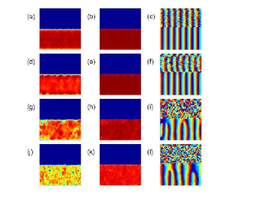
Figure 10: (Color online) Time development in the Gutzwiller approximation of a system with $J=0.045U$, $U_{12}=0.85U$, and $\mu=0.7U$, with wave vectors $(k/2,-k/2)$ where $k=7\pi/16$. Snapshots displayed in the different rows are taken at times (from top to bottom) $100/U$, $200/U$, $300/U$, and $4000/U$. Left column indicates total density $n$, middle column condensate density $n_{c}$, and right column the phase $\varphi$, of bosons of component 1. The corresponding quantities for component 2 are not shown, but are similar to the ones shown mirrored in the $x$ axis.

It is seen that the condensate densities behave very much like in the pure-condensate case. The time scale is vastly different due to the difference in tunneling matrix element $J$. In addition, it is seen that the total density is affected very little, and on the time scales we have simulated the system seems to be settling down into a phase separated steady state. The two fluids do not mix; the main effect of the KH instability is to excite vortices within the respective components. In the phase plots one can see vortices as phase singularities; they show up as zeros of the condensate density but the total density is not depleted. These are vortices filled with Mott insulating atoms, as previously described in Refs. wu2004 ; lundh2008b .

We next show a simulation at the point marked B in the phase diagram of Fig 8: $J=0.035U,U_{12}=0.85U$, and $\mu=0.7U$. This is still in the regime of two phase separated superfluids, but even closer to the Mott transition. Figure 11 shows the dynamics.

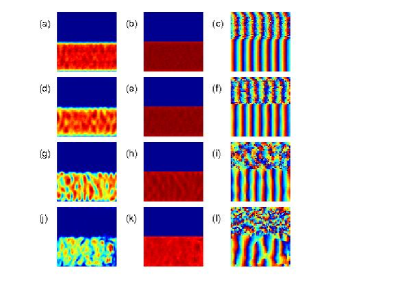
Figure 11: (Color online) Time development in the Gutzwiller approximation of a system with $J=0.035U$, $U_{12}=0.85U$, and $\mu=0.7U$, with wave vectors $(k/2,-k/2)$ where $k=7\pi/16$. Snapshots displayed in the different rows are taken at times (from top to bottom) $100/U$, $200/U$, $300/U$, and $4000/U$. Left column indicates total density $n$, middle column condensate density $n_{c}$, and right column the phase $\varphi$, of bosons of component 1. The corresponding quantities for component 2 are not shown, but are similar to the ones shown mirrored in the $x$ axis.

We see that the dynamics is in fact more rapid here than in the case of larger $J$. At times $t=200/U$ and $t=300/U$, a significant wave pattern develops in the condensate component, and at $t=1000/U$, the system contains many more vortices than in the case in Fig. 10. The total density is less affected, but exhibits some protruding features at the surface. Clearly, with a smaller condensate fraction, the threshold energy is smaller for modulation of condensate density and formation of vortices. Close to the transition, where the condensate density decreases rapidly towards zero, this overcomes the effect of the modest reduction of $J$.

VI Conclusions

In summary, we have studied the Kelvin-Helmholtz instability on the interface between two lattice Bose gases in relative motion. The instability is seen to be affected by three effects introduced by the lattice potential: broken translational symmetry, discreteness, and quantum fluctuations. Broken translational symmetry affects the instability in such a way that the excitation frequencies do not depend only on the relative velocity, but on the flow velocities of the two gases separately; the symmetric case of two counter-flowing gases is seen to be the most unstable situation. Second, the discreteness will stabilize slow relative currents, so that the instability is prevented if the relative velocity is low enough. Finally, strongly correlated physics affects the physics in such a way that a neighboring Mott insulating phase will prevent the two Bose systems from mixing after the Kelvin-Helmholtz instability is first excited. Close to the Mott phase transition, only the superfluid density will take part in the instability, but the total density will hardly be affected.

- (1) H. Hasegawa et al., Nature 430, 755 (2004).
- (2) R. Blaauwgeers et al., Phys. Rev. Lett. 89, 155301 (2002).
- (3) G. E. Volovik, JETP Lett. 75, 418 (2002).
- (4) D. S. Hall, M. R. Matthews, C. E. Wieman, and E. A. Cornell, Phys. Rev. Lett. 81, 1543 (1998).
- (5) J. Stenger et al., Nature 396, 345 (1998).
- (6) G. Modugno et al., Science 294, 1320 (2001).
- (7) H. Takeuchi et al., Phys. Rev. B 81, 094517 (2010).
- (8) N. Suzuki et al., Phys. Rev. A 82, 063604 (2010).
- (9) D. Jaksch et al., Phys. Rev. Lett. 81, 3108 (1998).
- (10) S. Powell, Phys. Rev. A 79, 053614 (2009).
- (11) M. Iskin, Phys. Rev. A 82, 033630 (2010).
- (12) A. L. Fetter, Annals of Physics 70, 67 (1972).
- (13) S. Chandrasekhar, Hydrodynamic and hydromagnetic stability, International series of monographs on physics (Dover Publications, New York, 1961).
- (14) R. A. Gerwin, Rev. Mod. Phys. 40, 652 (1968).
- (15) L. De Sarlo et al., Phys. Rev. A 72, 013603 (2005).
- (16) P. Ao and S. T. Chui, Phys. Rev. A 58, 4836 (1998).
- (17) E. Lundh and H. M. Nilsen, Phys. Rev. A 74, 063620 (2006).
- (18) H. M. Nilsen and E. Lundh, Phys. Rev. A 77, 013604 (2008).
- (19) J. Zakrzewski, Phys. Rev. A 71, 043601 (2005).
- (20) E. Lundh, Phys. Rev. A 84, 033603 (2011).
- (21) K. V. Krutitsky and P. Navez, Phys. Rev. A 84, 033602 (2011).
- (22) A. M. Rey et al., Journal of Physics B: Atomic, Molecular and Optical Physics 36, 825 (2003).
- (23) C. Wu, H. dong Chen, J. piang Hu, and S.-C. Zhang, Phys. Rev. A 69, 043609 (2004).
- (24) E. Lundh, EPL (Europhysics Letters) 84, 10007 (2008).