Computation of exterior moduli of quadrilaterals

Abstract.

We study the problem of computing the exterior modulus of a bounded quadrilateral. We reduce this problem to the numerical solution of the Dirichlet-Neumann problem for the Laplace equation. Several experimental results, with error estimates, are reported. Our main method makes use of an $hp$-FEM algorithm, which enables computations in the case of complicated geometry. For simple geometries, good agreement with computational results based on the SC Toolbox, is observed. We also use the reciprocal error estimation method introduced in our earlier paper to validate our numerical results. In particular, exponential convergence, in accordance with the theory of Babuška and Guo, is demonstrated.

1. Introduction

A bounded Jordan curve in the complex plane divides the extended complex plane $\mathbb{C}_{\infty}=\mathbb{C}\cup\{\infty\}$ into two domains $D_{1}$ and $D_{2}$, whose common boundary it is. One of these domains, say $D_{1}\,,$ is bounded and the other one is unbounded. The domain $D_{1}\,$ together with four distinct points $z_{1},z_{2},z_{3},z_{4}$ in $\partial D_{1}\,,$ which occur in this order when traversing the boundary in the positive direction, is called a quadrilateral and denoted by $(D_{1};z_{1},z_{2},z_{3},z_{4})\,$ [1, 17, 20, 22].

By Riemann’s mapping theorem, the domain $D_{1}\,$ can be mapped conformally onto a rectangle $f\colon D_{1}\to(0,1)\times(0,h)\,$ such that the four distinguished points are mapped onto the vertices of the rectangle $f(z_{1})=0\,,$ $f(z_{2})=1,$ $f(z_{3})=1+ih,$ $f(z_{4})=ih\,.$ The unique number $h$ is called the (conformal) modulus of the quadrilateral $(D_{1};z_{1},z_{2},z_{3},z_{4})\,$ [1, 17, 20, 22]. Apart from its theoretical significance in geometric function theory, the conformal modulus is closely related to certain physical quantities which also occur in engineering applications. In particular, the conformal modulus plays an important role in determining resistance values of integrated circuit networks (see e.g. [27, 28]). Similarly, one can map $D_{2}\,,$ the complementary domain, conformally $g\colon D_{2}\to(0,1)\times(0,k)\,$ such that the four boundary points are mapped onto the vertices of the rectangle $g(z_{1})=0\,,$ $g(z_{2})=1,$ $g(z_{3})=1+ik,g(z_{4})=ik\,$, reversing the orientation. Again the number $k$ is unique and it is called the exterior modulus of $(D_{1};z_{1},z_{2},z_{3},z_{4})\,.$ In practice, the computation of both the modulus and the exterior modulus is carried out by using numerical methods such as numerical conformal mapping. Mapping problems involving unbounded domains likewise are related to some well known engineering applications such as determining two dimensional potential flow around a cylinder, or an airfoil.

In the case of domains with polygonal boundary, numerical methods based on the Schwarz-Christoffel formula have been extensively studied, see [10]. One of the pioneers of numerical conformal mapping was D. Gaier [12], [26]. The literature and software dealing with numerical conformal mapping problems is very wide, see e.g. [10] and [27]. In our earlier paper [15] we applied an alternative approach which reduces the problem to the Dirichlet-Neumann problem for the Laplace equation. Thus any software capable of solving this problem may be used. We use the $hp$-FEM method for computing the modulus of a bounded quadrilateral and here we will apply the same method for the exterior modulus and another method, AFEM [7], for the sake of comparison, as in [15]. Our approach also applies to the case of domains bounded by circular arc boundaries as we will see below. It should be noted that while our method does not require finding the canonical conformal mapping, it is possible to construct the mapping from the potential function. An algorithm, with several numerical examples, is presented in [14]. An alternative to FEM would be to use numerical methods for integral equations. For recent work on numerical conformal mapping based on such an approach, see Nasser [24].

In particular, an important example of a quadrilateral $(D_{1};z_{1},z_{2},z_{3},z_{4})\,$ is the case when $D_{1}$ is a polygon with $z_{1},z_{2},z_{3},z_{4}\,$ as the vertices and its modulus was computed in [16] and this formula was also applied in [15]. Here we reduce its exterior modulus to the (interior) modulus by carrying out a suitable inversion which keep three vertices invariant and maps the exterior to the interior of a bounded plane region whose boundary consists of four circular arcs.

We apply here three methods to study our basic problem:

• The $hp$-FEM method introduced in [15] and its implementation by H. Hakula.

• The AFEM method of K. Samuelsson, see e.g. [7] and [15].

• The Schwarz-Christoffel Toolbox of T. Driscoll and N. Trefethen [9, 10, 31, 32].

The methods (1) and (2) are based on a reduction of the exterior modulus problem to the solution of the Dirichlet-Neumann problem for the Laplace equation in the same way as in [1] and [15] whereas (3) makes use of numerical conformal mapping methods. Note that [1] also provides a connection between the extremal length of a family of curves and its reciprocal, the modulus of a curve family, both of which are widely used in the geometric function theory.

We describe the high-order $p$-, and $hp$-finite element methods and report the results of numerical computation of the exterior moduli of a number of quadrilaterals. In the $p$-method, the unknowns are coefficients of some polynomials that are associated with topological entities of elements, nodes, sides, and the interior. Thus, in addition to increasing accuracy through refining the mesh, we have an additional refinement parameter, the polynomial degree $p$. For an overview of the $hp$-method, see e.g. Babuška and Suri [6]. A more detailed exposition of the methods is given in [29, 30].

Our study is structured according to a few particular cases. We start out with the case when the quadrilateral is the complement of a rectangle and the vertices are the distinguished points of the quadrilateral. In this case we have the formula of P. Duren and J. Pfaltzgraff [11] to which we compare the accuracy of each of the above methods (1)-(3). Then we consider the problem of minimizing the exterior modulus of a trapezoid with a fixed height $h$ and fixed lengths for the pair of parallel opposite sides and present a conjecture supported by our experiments. We also remark that the case of symmetric hexagons can be dealt with the Schwarz-Christoffel transformation and relate its exterior modulus to a symmetry property of the modulus of a curve family. Finally, we study the general case and present comparisons of methods (1)-(3) for this case as well. SC Toolbox does not have a built in function for computing the exterior modulus. However, we use the function extermap, and an auxiliary Möbius transformation, to map the exterior of a quadrilateral $(D;a,b,c,d)$ conformally onto the upper half-plane so that the boundary points $a,b,c$ and $d$ are mapped to the points $\infty,-1,0$ and $t>0$, respectively. Then the exterior modulus of the quadrilateral is $\tau(t)/2$, where $\tau$ is the Teichmüller modulus function (see [2] and 2.2 below). We use the MATLAB code from [2] to compute values of $\tau(t)$, $t>0$.

Our computational workhorse, the $hp$-FEM algorithm implemented in Mathematica, is used in all cases involving general curved boundaries. We demonstrate that nearly the optimal rate of convergence, $C_{1}\exp(-C_{2}N^{1/3})$ in terms of the number $N$ of unknowns as predicted by the results of Babuška and Guo [4], is attained in a number of tests cases. Our results are competitive with the survey results on $hp$-adaptive algorithms reported by Mitchell and MacClain [23] for the L-shaped domain.

At the end of the paper we present conclusions concerning the performance of these methods and our discoveries.

2. Preliminaries

In this section we give reference results which can be used in obtaining error estimates. We also present some geometric identities which are required in our computations.

2.1. The hypergeometric function and complete elliptic integrals

Given complex numbers $a,b,$ and $c$ with $c\neq 0,-1,-2,\ldots$, the Gaussian hypergeometric function is the analytic continuation to the slit plane $\mathbb{C}\setminus[1,\infty)$ of the series

(2.1) $$F(a,b;c;z)={}_{2}F_{1}(a,b;c;z)=\sum_{n=0}^{\infty}\frac{(a,n)(b,n)}{(c,n)}\frac{z^{n}}{n!}\,,\>\>|z|<1\,.$$

Here $(a,0)=1$ for $a\neq 0$, and $(a,n)$ is the shifted factorial function or the Appell symbol

$$(a,n)=a(a+1)(a+2)\cdots(a+n-1)$$

for $n\in\mathbb{N}\setminus\{0\}$, where $\mathbb{N}=\{0,1,2,\ldots\}$ and the elliptic integrals $\hbox{\ff K}(r),\hbox{\ff K}^{\prime}(r)$ of the first kind are

$$\hbox{\ff K}(r)=\frac{\pi}{2}F(1/2,1/2;1;r^{2}),\qquad\hbox{\ff K}^{\prime}(r)=\hbox{\ff K}(r^{\prime}),\text{ and }r^{\prime}=\sqrt{1-r^{2}},$$

and the elliptic integrals $\hbox{\ff E}(r),\hbox{\ff E}^{\prime}(r)$ of the second kind are

$$\hbox{\ff E}(r)=\frac{\pi}{2}F(1/2,-1/2;1;r^{2}),\qquad\hbox{\ff E}^{\prime}(r)=\hbox{\ff E}(r^{\prime}),\text{ and }r^{\prime}=\sqrt{1-r^{2}}.$$

Some basic properties of these functions can be found in [2, 25].

2.2. The modulus of a curve family

For a family of curves $\Gamma$ in the plane, we use the notation $\mbox{\sf M}(\Gamma)$ for its modulus [22]. For instance, if $\Gamma$ is the family of all curves joining the opposite $b$-sides within the rectangle $[0,a]\times[0,b],a,b>0,$ then $\mbox{\sf M}(\Gamma)=b/a\,.$ If we consider the rectangle as a quadrilateral $Q$ with distinguished points $a+ib,ib,0,a$ we also have $\mbox{\sf M}(Q;a+ib,ib,0,a)=b/a\,,$ see [1, 22] . Given three sets $D,E,F$ we use the notation $\Delta(E,F;D)$ for the family of all curves joining $E$ with $F$ in $D\,.$

Next consider another example, which is important for the sequel. For $t>0$ let $E=[-1,0]$, $F=[t,\infty)$ and let $\Delta_{t}$ be the family of curves joining $E$ and $F$ in the upper half-plane ${\mathbb{C}}_{+}=\{z\in\mathbb{C}:\,\,{\rm Im}\,z>0\}\,.$ Then [2], we have

$$\mbox{\sf M}(\Delta_{t})=\tau(t)/2\,;\quad\tau(t)=2\frac{\hbox{\ff K}(1/\sqrt{1+t})}{\hbox{\ff K}(\sqrt{t/(1+t)})}\,.$$

2.3. The Duren-Pfaltzgraff formula [11, Theorem 5]

For $k\in(0,1)$ write

$$\psi(k)=\frac{2(\hbox{\ff E}(k)-(1-k)\hbox{\ff K}(k))}{\hbox{\ff E}^{\prime}(k)-k\hbox{\ff K}^{\prime}(k)}\,.$$

Then $\psi\colon(0,1)\to(0,\infty)$ defines an increasing homeomorphism with limiting values $0,\infty$ at $0,1$, respectively. In particular, $\psi^{-1}\colon(0,\infty)\to(0,1)$ is well-defined. Let $R$ be a rectangle with sides of lengths $a$ and $b$, respectively, and let $\Gamma$ be the family of curves lying outside $R$ and joining the opposite sides of length $b\,.$ Then

(2.2) $$\mbox{\sf M}(\Gamma)=\frac{\hbox{\ff K}^{\prime}(k)}{2\hbox{\ff K}(k)}\,,\quad\textrm{where}\,\,k=\psi^{-1}(a/b)\,.$$

This formula occurs in different contexts. For instance, W.G. Bickley ([8], (1.17) p. 86) used it in the analysis of electric potentials and W. von Koppenfels and F. Stallmann ([19], (4.2.31) and (4.2.63)) established it in conformal mapping problems. As far as we know, Duren and Pfaltzgraff were the first authors to connect this formula with the exterior modulus of a quadrilateral.

2.4. Mapping unbounded onto bounded domains

The transformation $z\mapsto z/|z|^{2}$ maps the complement of the closed unit disk onto the unit disk. This transformation is an anticonformal mapping and it maps the complement of a polygonal quadrilateral with vertices $a,b,c,d$ with $|b|=|c|=|d|=1$ onto a bounded domain, bounded by four circular arcs. Note that the points $b,c,d$ remain invariant under this transformation. See Figure -1259. Here we also make use of the well-known formula for the center of the circle through three given points.

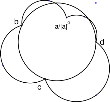
Figure -1259. Polygonal quadrilateral before (left) and after (right) the inversion transformation $z\mapsto z/|z|^{2}$. Note that the points $b,c,d$ on the unit circle remain invariant.

2.5. The Dirichlet-Neumann problem

The following problem is known as the Dirichlet-Neumann problem. Let $D$ be a region in the complex plane whose boundary $\partial D$ consists of a finite number of regular Jordan curves, so that at every point, except possibly at finitely many points, of the boundary a normal is defined. Let $\partial D=A\cup B$ where $A,B$ both are unions of Jordan arcs. Let $\psi_{A},\psi_{B}$ be a real-valued continuous functions defined on $A,B$, respectively. Find a function $u$ satisfying the following conditions:

1. $u$ is continuous and differentiable in $\overline{D}$.

2. $u(t)=\psi_{A}(t),\qquad\textrm{ for all}\,\,t\in A$.

3. If $\partial/\partial n$ denotes differentiation in the direction of the exterior normal, then

   $$\frac{\partial}{\partial n}u(t)=\psi_{B}(t),\qquad\textrm{ for all}\,\,t\in B.$$

2.6. Modulus of a quadrilateral and Dirichlet integrals

One can express the modulus of a quadrilateral $(D;z_{1},z_{2},z_{3},z_{4})$ in terms of the solution of the Dirichlet-Neumann problem as follows. Let $\gamma_{j},j=1,2,3,4$ be the arcs of $\partial D$ between $(z_{4},z_{1})\,,$ $(z_{1},z_{2})\,,$ $(z_{2},z_{3})\,,$ $(z_{3},z_{4}),$ respectively. If $u$ is the (unique) harmonic solution of the Dirichlet-Neumann problem with boundary values of $u$ equal to $0$ on $\gamma_{2}$, equal to $1$ on $\gamma_{4}$ and with $\partial u/\partial n=0$ on $\gamma_{1}\cup\gamma_{3}\,,$ then by [1, p. 65/Thm 4.5]:

(2.3) $$\mbox{\sf M}(D;z_{1},z_{2},z_{3},z_{4})=\iint_{D}|\triangledown u|^{2}\,dx\,dy.$$

2.7. The reciprocal identity

Given a quadrilateral $Q=(D;z_{1},z_{2},z_{3},z_{4})$ we call sometimes $\tilde{Q}=(D;z_{2},z_{3},z_{4},z_{1})$ the conjugate quadrilateral. It a simple basic fact that

(2.4) $$\mbox{\sf M}(Q)\mbox{\sf M}(\tilde{Q})=1\,.$$

It was suggested in [16] and [15] that the quantity

(2.5) $$r(Q)=|\mbox{\sf M}(Q)\mbox{\sf M}(\tilde{Q})-1|\,$$

might serve as a useful error characteristic. We will continue to use this also in our work.

2.8. The $hp$-FEM method and meshing

In this paper, we use the $hp$-FEM method for computing for the exterior modulus of a quadrilateral. For a general description of our method, see [15]. Proper treatment of corner singularities is handled with the following two-phase algorithm, typically recursive, where triangles can be replaced by quadrilaterals or a mixture of both:

1. Generate an initial mesh (triangulation) where the corners are isolated with a fixed number of triangles depending on the interior angle, $\theta$ so that the refinements can be carried out independently:

   1. $\theta\leq\pi/2$: one triangle,

   2. $\pi/2<\theta\leq\pi$: two triangles, and

   3. $\pi<\theta$: three triangles.

2. Every triangle attached to a corner is replaced by a refinement, where the edges incident to the corner are split as specified by the scaling factor $\alpha$. This process is repeated recursively until the desired nesting level $\nu$ is reached. The resulting meshes are referred to as $(\alpha,\nu)$-meshes. Note that the mesh may include quadrilaterals after refinement.

Since the choice of the initial mesh affects strongly the refinement process, it is advisable to test with different choices. Naturally, one would want the initial mesh to be minimal, that is, having the smallest possible number of elements yet providing support for the refinement. This is why initial meshes are sometimes referred to as minimal meshes.

Figure -1258. A sample geometry and the corresponding initial mesh. Note that the three-element -rule is satisfied at every corner.

Figure -1257. A detail of the initial mesh and the final $(0.15,14)$-mesh used in the actual computation.

In Figure -1258 a challenging example is shown. In this case the large variation of the edge lengths is addressed by adding a refinement step to the construction of the initial mesh. A detail of the initial mesh is given in Figure -1257 along with the final mesh.

3. The case of a rectangle

The first tests with the $hp$-FEM software were made for the case of the exterior modulus of a rectangle and checked against the Duren-Pfaltzgraff formula (2.2). For a convenient parametrization of the computation, the vertices of the rectangle were chosen to be the points $1,e^{it},-1,-e^{it},t\in(0,\pi/2]$ of the unit circle. In this case, the ”interior” modulus of the rectangle is $\tan(t/2)\,.$ It is equal to the modulus of the family of curves joining the sides $[1,e^{it}]$ and $[-1,-e^{it}]$ and lying in the interior of the rectangle. The formula (2.2) now gives the corresponding exterior modulus as

$$\frac{\hbox{\ff K}^{\prime}(k)}{2\hbox{\ff K}(k)}\,,\qquad k=\psi^{-1}\bigg{(}\frac{1}{\tan(t/2)}\bigg{)}.$$

For the computation, we carried out the inversion $z\mapsto 1/\overline{z}$ in the unit circle which keep all the points of the unit circle fixed and transforms the exterior modulus problem for the rectangle to the ”interior” modulus problem of a plane domain bounded by four circular arcs, see Figure -1256. These circular arcs are the images of the sides of the rectangle under the inversion. The results turned out to be quite accurate, with a typical relative error of the order $10^{-10}\,.$

Table 1. Exact values of the moduli of $Q(1,e^{it},-1,-e^{it})$ given by (2.2) and the errors of computational results of the $hp$-method, $p=20,$ the AFEM method and the SC Toolbox. The errors are obtained by comparing with the exact formula (2.2). The errors are given as $\lceil\log_{10}|\mathrm{error}|\rceil$.

$k$	exact($t=k\pi/12$)	Error[hpFEM]	Error[AFEM]	Error[SCT]
$1$	$1.50290233467$	$-9$	$-6$	$-9$
$2$	$1.31044063554$	$-9$	$-6$	$-9$
$3$	$1.20035166917$	$-9$	$-6$	$-10$
$4$	$1.12114255114$	$-10$	$-6$	$-9$
$5$	$1.05681535228$	$-10$	$-6$	$-13$
$6$	$1.$	$-10$	$-6$	$-15$

(a) $k=1$

(b) $k=2$

(c) $k=3$

(d) $k=4$

(e) $k=5$

(f) $k=6$

Figure -1256. Circular arc domains used for the $hp$-FEM computations of the values in Table 1. The scale varies from picture to picture.

Figure -1255. The circular arc domains of Figure -1256 in the same scale.

4. Side sliding conjecture

4.1. The side sliding problem

Consider the problem of finding the minimal exterior modulus of the polygonal quadrilateral with vertices $0,1,a=t+ih,b=t-s+ih$ when $h,s>0$ are fixed and $t$ varies. We consider the question of computing the modulus of the family $\Gamma$ of curves joining the opposite sides $[1,a]$ and $[b,0]$ outside the quadrilateral. Our first step is to reduce the problem to an equivalent problem such that three of the points are on the unit circle. Note that this setting is valid only if $z_{0}$ is inside the quadrilateral. Indeed, for every choice of $h$ and $s$ this condition defines an upper limit for the value of $t$.

4.2. Side sliding conjecture

The least valueof the exterior modulus is attained when $t=(1+s)/2\,.$ For $t\leq(1+s)/2\,$ the modulus is a decreasing function of $t\,.$

4.3. Numerical experiments on side sliding conjecture

In Figure -1254 we show a graph of the exterior module as a function of the parameter $t\in[0.5,2.5]$, when $h=1,s=2$. The computation was carried out with SC Toolbox, $hp$-FEM, and AFEM and for the range of computed values, the respective graphs coincide. For the SC Toolbox and the $hp$-FEM the reciprocal estimate for the error was smaller than $10^{-8}$ and for AFEM $10^{-5}$.

Figure -1254. Side Sliding Conjecture: Dependence of the exterior modulus on parameter $t$ with $h=1,s=1$. Maximum is reached at $t=(1+s)/2=1$, as predicted by the conjecture.

5. The case of a symmetric hexagon

Suppose that $Q(a,b,0,1)$ is a quadrilateral in the upper half plane. Then the closed polygonal line $a,b,0,\overline{b},\overline{a},1,a$ defines a hexagon $H=Q\cup\overline{Q}$ symmetric with respect to the real axis. Map the complement of $H$ onto $\mathbb{C}\setminus\{-1-t,1+t\}$ by a conformal map $h$ such that $h(0)=-1-t,h(b)=h(\overline{b})=-1,h(a)=h(\overline{a})=1,h(1)=1+t$ where $t>0$ depends on the point configuration $a,b,0,1\,.$ It is clear by symmetry that

(5.1) $$2\mbox{\sf M}(\Delta^{+})=\mbox{\sf M}(\Delta)$$

where

$$\Delta=\Delta\big{(}[-1-t,-1],[1,1+t];\mathbb{C}\big{)}\,\,\textrm{and}\,\,\Delta^{+}=\Delta\big{(}[-1-t,-1],[1,1+t];\{z:\mathrm{Im}\,z>0\}\big{)}\,.$$

Because of the conformal invariance of the modulus we also have

(5.2) $$2\mbox{\sf M}\big{(}h^{-1}(\Delta^{+})\big{)}=\mbox{\sf M}\big{(}h^{-1}(\Delta)\big{)}\,.$$

Applying this formula with (2.2) we see that

(5.3) $$\mbox{\sf M}(\Gamma_{+})=\frac{\hbox{\ff K}^{\prime}(k)}{4\,\hbox{\ff K}(k)}\,,\quad k=\psi^{-1}\bigg{(}\frac{1}{2h}\bigg{)}\,,$$

where for $h>0$,

(5.4) $$\Gamma_{+}=\Delta\big{(}[0,ih],[1,1+ih];{\mathbb{C}}_{+}\setminus[0,1]\times[0,h]\big{)}\,.$$

This formula can be checked by using the SC Toolbox to construct the above conformal mapping $h\,.$ The tests we carried out for $h=0.2,0.3,0,4$ and $0.5$ In these cases the reciprocal estimate for error was smaller than $10^{-9}\,.$

6. General quadrilateral

The exterior modulus of the quadrilateral $Q$ with vertices $a,b,c,d$ is considered in this section, i.e., we compute

$$\iint_{Q}\,|\nabla u|^{2}\,dx\,dy$$

over the complement of the quadrilateral when $u$ is the solution of the Laplace equation in the complement of the quadrilateral with Dirichlet values $1$ and $0$ on the sides $[b,c]$ and $[d,a]\,,$ respectively, and the Neumann value $0$ on the sides $[a,b]$ and $[c,d]\,.$ Here we allow the boundary of the quadrilateral $\partial Q$, be a parametrized curve $\gamma(t)$, $t\in[-1,1]$.

(a) Exterior domain with radius $>1000000$.

(b) Zoom of the mesh in the case of a circle.

(c) Zoom of the mesh in the case of a square.

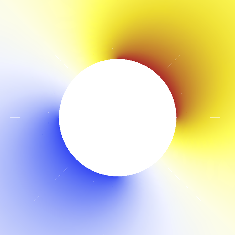
(d) Zoom of the potential in the case of a circle. Reciprocal error $\sim 8.8\cdot 10^{-10}$

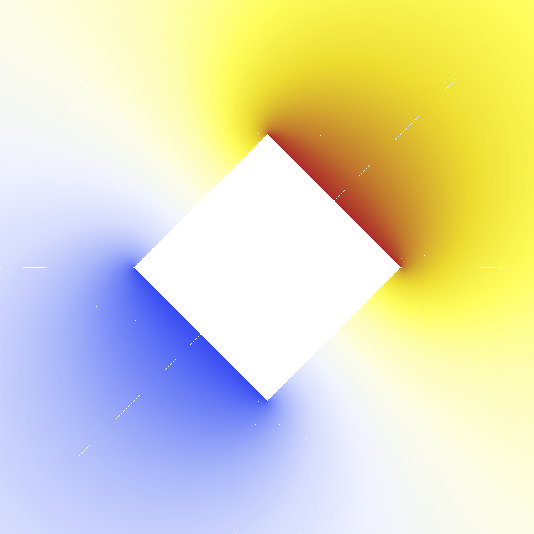
(e) Zoom of the potential in the case of a square. Reciprocal error $\sim 6.3\cdot 10^{-10}$

Figure -1253. Exterior modulus over the exterior domain.

In Figure -1253 an overview of the standard FEM approach is given. Using higher-order elements one can stretch the domain without introducing significant number of elements. Singularities at the corner point must be accounted for in the grading of the mesh. Since both the circle and the square cases are symmetric, the exterior modulus is exactly 1, and furthermore the potential value at infinity or the far-field value is exactly 1/2.

6.1. Quadrilaterals A and B

In Tables 2, 3, and 6 results on two polygonal quadrilaterals

• Quadrilateral A: $\{0,1,({28}/{25},{69}/{50}),(-{19}/{25},{21}/{25})\}$,

• Quadrilateral B: $\{0,1,({42}/{25},4),(-{3}/{25},{21}/{25})\}$,

are presented. The exterior modulus has been computed using three methods as an equivalent interior modulus problem, and also in truncated domain. In the interior case, both SC Toolbox and $hp$-FEM give similar results, but AFEM in its standard setting does not reach the desired accuracy. This is probably due to the adaptive scheme failing in the presence of cusps in the domain. Tables 2 and 3 indicate that large exterior angles are the most significant source of errors in the FEM solutions, as expected. In the rather benign setting of the Quadrilateral A, SC Toolbox and both the internal and external $hp$-FEM versions have the same accuracy, but in the case of Quadrilateral B, we see gradual loss of accuracy in the FEM solutions.

6.2. Quadrilaterals C and D

Finally, we consider two flower domains, that is, quadrilateral domains with the boundary $\gamma(t)=r(t)e^{it}\,,\,r(t)=4/5+(1/5)\cos(n\pi t)$ and corners at $t=-1,-1/4,0,1/2$. For the Quadrilateral C we choose $n=4$ and for D we choose $n=8$. These domains have the useful property that the exterior problem can easily be converted to a corresponding interior problem of the domain with boundary $1/\overline{\gamma(t)}$. Since these domains cannot be handled using the SC Toolbox, we take the interior solution as the reference. Tables 4 and 5 show that we can obtain results of high accuracy also in traditionally challenging domains.

It turns out that besides the actual value of the exterior modulus one can also determine the value of the far-field potential. Either one can determine the value of the potential at the reflection point of the interior problem, i.e., at the origin, or simply evaluate the solution of the exterior problem at the farthest point. Remarkably, the truncated domain results agree well with the (theoretically) exact results of the equivalent inner modulus problems (Table 6). In Figures -1252–-1249 we show comparisons of the interior and exterior potential fields. For the two polygonal quadrilaterals, the corresponding contour lines and the location of the origin in the interior case are indicated. In the general case, prediction of the far-field value based solely on geometric arguments is an open problem.

We note, that for both Quadrilateral C and D, the interior and exterior capacities are equal. This invariance is new and has not been reported in the literature before. It is crucial that the four corners are chosen from extremal points, that is, local minima and maxima of the radius.

Method	Exterior Modulus	Error (2.5)	Relative Error
SC Toolbox	0.9923416323	-9	–
AFEM	0.9923500126	-4	-5
$hp$-FEM (Interior)	0.9923416332	-9	-9
$hp$-FEM (Exterior)	0.9923416332	-9	-9

Table 2. Quadrilateral A: $\{0,1,({28}/{25},{69}/{50}),(-{19}/{25},{21}/{25})\}$. The values obtained with SC Toolbox are used as reference. The errors are given as $\lceil\log_{10}|\mathrm{error}|\rceil$.

Method	Exterior Modulus	Error (2.5)	Relative Error
SC Toolbox	0.9592571721	-9	–
AFEM	0.9593012739	-4	-4
$hp$-FEM (Interior)	0.9592571731	-8	-8
$hp$-FEM (Exterior)	0.9592572007	-7	-7

Table 3. Quadrilateral B: $\{0,1,({42}/{25},4),(-{3}/{25},{21}/{25})\}$. The values obtained with SC Toolbox are used as reference. The errors are given as $\lceil\log_{10}|\mathrm{error}|\rceil$.

Method	Exterior Modulus	Error (2.5)	Relative Error
$hp$-FEM (Interior)	0.8196441884805177	-14	–
$hp$-FEM (Exterior)	0.8196441926483611	-8	-8

Table 4. Quadrilateral C: $\gamma(t)=r(t)e^{it},r(t)=4/5+(1/5)\cos(4\pi t)$ and corners at $t=-1,-1/4,0,1/2$. The values obtained with $hp$-FEM (Interior) are used as reference. The errors are given as $\lceil\log_{10}|\mathrm{error}|\rceil$.

Method	Exterior Modulus	Error (2.5)	Relative Error
$hp$-FEM (Interior)	0.9122187602015264	-10	–
$hp$-FEM (Exterior)	0.9122187628550672	-8	-8

Table 5. Quadrilateral D: $\gamma(t)=r(t)e^{it},r(t)=4/5+(1/5)\cos(8\pi t)$ and corners at $t=-1,-1/4,0,1/2$. The values obtained with $hp$-FEM (Interior) are used as reference. The errors are given as $\lceil\log_{10}|\mathrm{error}|\rceil$.

Quadrilateral	$hp$-FEM (Interior)	$hp$-FEM (Exterior)	Relative Error
A	0.5281867366243582	0.5281867468410989	-7
B	0.6659476737428786	0.6659476800244547	-8
C	0.5873283399651075	0.5873283469398137	-7
D	0.5398927341965689	0.5398927414203410	-7

Table 6. Comparison of the computed values of the potential at infinity. The errors are given as $\lceil\log_{10}|\mathrm{error}|\rceil$.

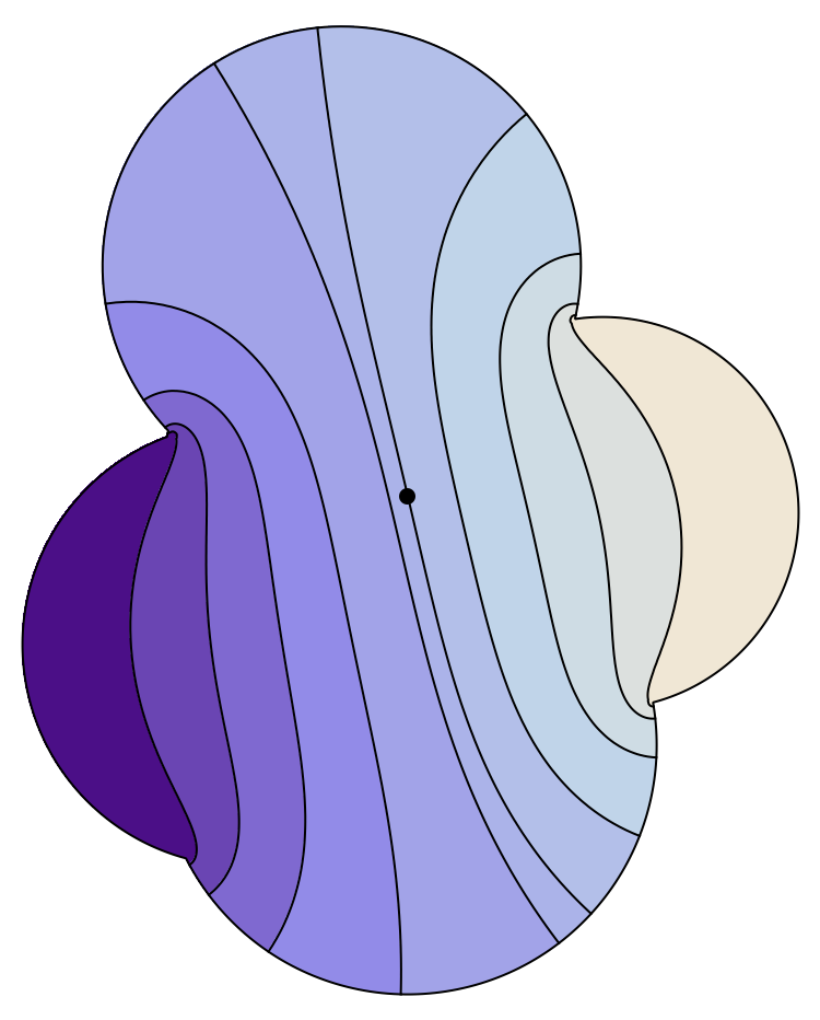
(a) Contours of the inner problem. Origin is indicated with a dot.

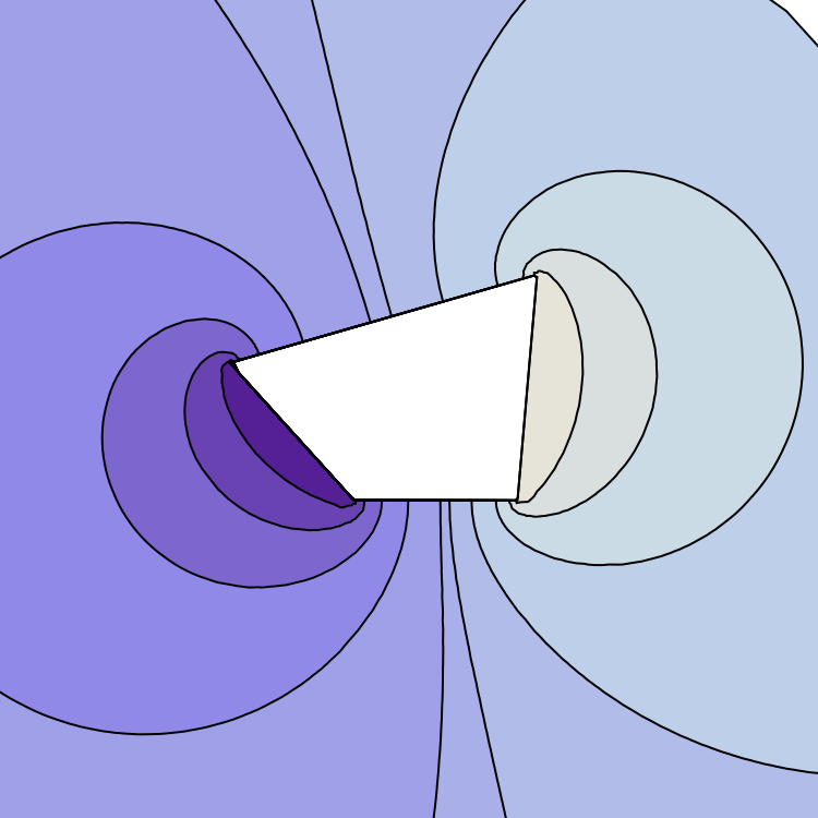
(b) Contours of the outer problem. Note the contours extending to infinity.

Figure -1252. Quadrilateral A: Correspondence of the potential contours between the inner (A) and outer (B) solutions. Shown are the potential levels $u(z)=0,1/10,\ldots,1$, and $u(0)$. Corresponding contours can be identified by matching the shadings of the regions in between.

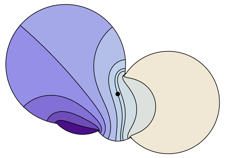
(a) Contours of the inner problem. Origin is indicated with a dot.

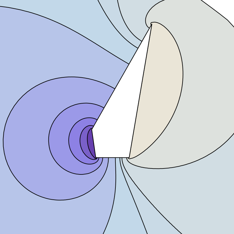
(b) Contours of the outer problem. Note the contours extending to infinity.

Figure -1251. Quadrilateral B: Correspondence of the potential contours between the inner (A) and outer (B) solutions. Shown are the potential levels $u(z)=0,1/10,\ldots,1$, and $u(0)$. Corresponding contours can be identified by matching the shadings of the regions in between.

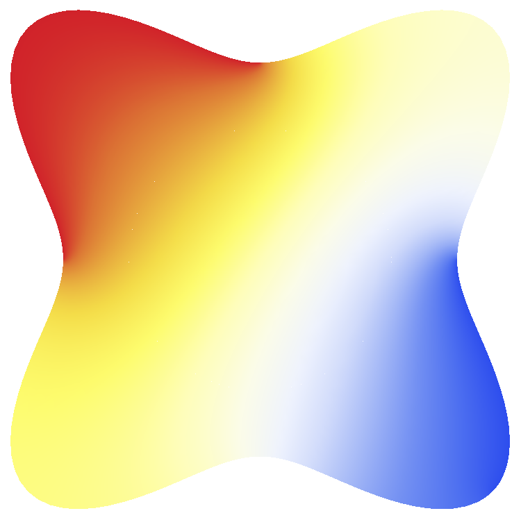
(a) Potential field of the inner problem.

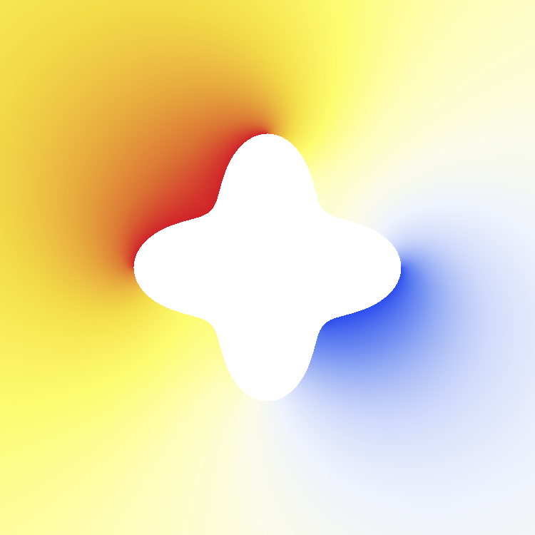
(b) Potential field of the outer problem.

Figure -1250. Quadrilateral C: The potential field of the inner (A) and outer (B) solutions.

(a) Potential field of the inner problem.

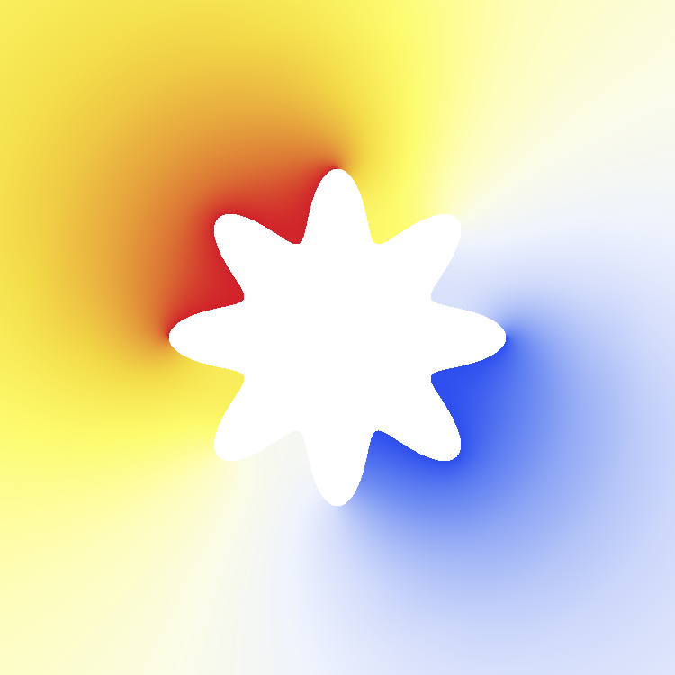
(b) Potential field of the outer problem.

Figure -1249. Quadrilateral D: The potential field of the inner (A) and outer (B) solutions.

7. Performance Considerations

In this section we study the performance of our approach in terms of computational cost in time and storage requirements, and convergence of the capacity, which is shown to be exponential. Here we consider the Quadrilateral D defined above, and compare the interior and exterior problems. This comparison is reasonable, since due to the new invariance, the interior and exterior problems can be solved using exactly the same the geometry and thus the singularities are of the same kind.

7.1. Convergence

All experiments have been computed using $(\alpha,\nu)$-meshes, with $\alpha=0.15$, and $\nu=\min(16,p_{\max})$, where 16 is dictated by double precision. This choice allows us to compare two elemental $p$-distributions, namely the constant $p=p_{\max}$, and the graded $p$-vector where the elemental $p$ increases per element layer away from the singularity, e.g., from $p=1$ up to $p=p_{\max}$. The $p_{\max}$ has been chosen so that the relative error in both approaches is roughly the same and in accordance with the results resported above, $p_{\max,I}=18$ and $p_{\max,E}=22$, for the interior and exterior problems, respectively.

The optimal rate of convergence of the relative error in capacity is

$$\sim C_{1}\exp(-C_{2}\,N^{1/3}),$$

where $N$ is the number of unknowns and $C_{i}$ are coefficients independent of $N$ [29]. In Figure -1248 the convergence plots corresponding to both $p$-distributions are shown using two different scalings: (A) in standard loglog-scale, and (B) in semilog-scale with $N^{1/3}$ as the abscissa. The first plot shows that solutions to both problems converge exponentially, but the latter one shows that the exterior approach is not as efficient as the interior one. Using linear fitting of logarithmic data, we find convergence rates of type $N^{1/\beta}$, with $\beta_{I,c}=3.72$, $\beta_{E,c}=3.8$, $\beta_{I,g}=3.41$, and $\beta_{E,g}=3.55$, where the indeces $c$ and $g$ refer to constant and graded polynomial distributions, respectively.

Two observations should be noted: a) faster convergence rate does not imply more accurate results; b) the convergence behaviour becomes less stable as $p>\nu$ as the refinement strategy is changed.

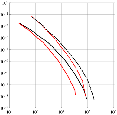
(a) Loglog-scale: relative error in capacity vs $N$.

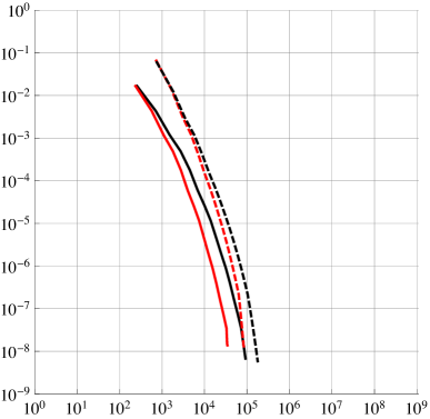
(b) Semilog-plot: relative error in capacity vs $N^{1/3}$.

Figure -1248. Quadrilateral D: Convergence of the relative error in capacity. Constant $p$: Black, Graded $p$: Red; Interior problem: Solid line; Exterior problem: Dashed line. The number of unknowns is $N$.

$p$	$N$	Meshing	Integration	(Assembly)	Solve	Total
4	1505	1	2	(0)	0	3
8	10049	4	14	(4)	4	22
12	31777	11	44	(14)	14	69
16	72833	21	136	(52)	42	199

(a) Interior problem.

$p$	$N$	Meshing	Integration	(Assembly)	Solve	Total
4	3456	4	2	(0)	0	6
8	17792	13	19	(6)	3	35
12	49152	26	63	(23)	10	99
16	103680	47	210	(80)	30	287

(b) Exterior problem.

Table 7. Quadrilateral D: Time spent in the solution process. All times are seconds as reported by Mathematica’s Timing-function. Time spent in assembly of the linear system is included in that of integration. (Apple Mac Pro 2009 Edition 2.26 GHz, Mathematica 8.0.4)

7.2. Time

Averaged timing results over a set of 30 runs with constant $p$-distribution are shown in Table 7. Note that the hierarchic nature of the problem has not been taken into account here and runs for different values of $p$ have been independent. In our implementation the numerical integration is the most expensive part. The numerical integration routines are based on a matrix-matrix multiplication formalism which is highly efficient on terms of flops per memory access, and benefits from BLAS-level parallelism on our test machine with eight cores; Apple Mac Pro 2009 Edition 2.26 GHz, Mathematica 8.0.4. The time spent in assembling the matrix is included in the integration time. Mathematica does not support pre-allocation of sparse matrix structures or autosumming initialization which leads to a lot of reallocation of sparse matrices.

Interestingly, the time spent on direct solution of the systems is shorter for the exterior problem for problems of comparable size. In our opinion this is the result of the ordering heuristic used by Mathematica being more efficient over ring domains.

8. Conclusions

In this study we have shown that three different algorithms, AFEM, SC Toolbox and $hp$-FEM, can all be effectively used for computation of the exterior modulus of a bounded polygonal quadrilateral. As far as we know, there are very few numerical or theoretical results on the exterior modulus in the literature. The problem is first reduced to a Dirichlet-Neumann problem for the Laplace equation. In our earlier paper [15] we introduced the reciprocal identity as an error estimate for the inner modulus computation of a quadrilateral and here we demonstrate that the same method applies to error estimation for the exterior modulus as well. We compare our numerical results to the analytic Duren-Pfaltzgraff formula for the exterior modulus of a rectangle and observe that our results agree with it. Moreover, in this case the analytic formula yields results that are within the limits provided by the reciprocal error estimate from our computational results. The reciprocal error estimate is also applied to study, for the case of polygonal quadrilaterals, the accuracy of the Schwarz-Christoffel toolbox and the AFEM method, and mutual accuracy comparisons are given. Finally, for the case of quadrilaterals with curvilinear boundary, where these two methods do not apply, we give results obtained by the $hp$-FEM method, and their error estimates based on the relative error and the reciprocal error estimate. In this case we also analyze the dependence of the accuracy on the number of degrees of freedom and demonstrate nearly optimal convergence, compatible with the theory of Babuška and Guo [4].

A problem of independent interest is the value of the potential function at infinity. We study this problem for the exterior modulus of a polygonal quadrilateral and solve it by mapping the exterior domain onto a bounded domain by inversion and then computing the value of the potential function of the corresponding interior modulus problem at the image point of the point at infinity.

Acknowledgements. The research of Matti Vuorinen was supported by the Academy of Finland, Project 2600066611. The authors are indebted to the referees for their helpful remarks.

References

- [1] L.V. Ahlfors, Conformal invariants: topics in geometric function theory. McGraw-Hill Book Co., 1973.
- [2] G.D. Anderson, M.K. Vamanamurthy and M. Vuorinen, Conformal invariants, inequalities and quasiconformal mappings. Wiley-Interscience, 1997.
- [3] S. Axler, P. Bourdon, and W. Ramey, Harmonic Function Theory. Graduate Texts in Mathematics, 2nd ed., Springer, 2001.
- [4] I. Babuška and B. Guo, Regularity of the solutions of elliptic problems with piecewise analytical data, parts I and II. SIAM J. Math. Anal., 19, (1988), 172–203 and 20, (1989), 763–781.
- [5] I. Babuška and B. Guo, Approximation properties of the -version of the finite element method. Comp. Meth. Appl. Mech. Engr., 133, (1996), 319–346.
- [6] I. Babuška and M. Suri, The P and H-P versions of the finite element method, basic principles and properties. SIAM Review 36 (1994), 578–632.
- [7] D. Betsakos, K. Samuelsson and M. Vuorinen, The computation of capacity of planar condensers. Publ. Inst. Math. 75 (89) (2004), 233–252.
- [8] W.G. Bickley, Two-dimensional potential problems for the space outside a rectangle. Proc. Lond. Math. Soc., Ser. 2, (37) (1932), 82–105.
-
[9]
T.A. Driscoll,
Schwarz-Christoffel toolbox for MATLAB,
http://www.math.udel.edu/~driscoll/SC/ - [10] T.A. Driscoll and L.N. Trefethen, Schwarz-Christoffel mapping. Cambridge Monographs on Applied and Computational Mathematics, 8. Cambridge University Press, Cambridge, 2002.
- [11] P. Duren and J. Pfaltzgraff, Robin capacity and extremal length. J. Math. Anal. Appl. 179 (1993), no. 1, 110–119.
- [12] D. Gaier, Konstruktive Methoden der konformen Abbildung. (German) Springer Tracts in Natural Philosophy, Vol. 3 Springer-Verlag, Berlin, 1964.
- [13] W.J. Gordon and C.A. Hall, Transfinite element methods: blending function interpolation over arbitrary curved element domains. Numer. Math. 21 (1973), 109–129.
- [14] H. Hakula, T. Quach and A. Rasila, Conjugate Function Method for Numerical Conformal Mappings. J. Comput. Appl. Math. 237 (2013), no. 1, 340–353.
- [15] H. Hakula, A. Rasila, and M. Vuorinen, On moduli of rings and quadrilaterals: algorithms and experiments. SIAM J. Sci. Comput. 33 (2011), 279–302 (24 pages), DOI: 10.1137/090763603, arXiv:0906.1261 [math.NA].
- [16] V. Heikkala, M.K. Vamanamurthy and M. Vuorinen, Generalized elliptic integrals. Comput. Methods Funct. Theory 9 (2009), 75–109. arXiv math.CA/0701436.
- [17] P. Henrici, Applied and Computational Complex Analysis, vol. III, Wiley-Interscience, 1986.
- [18] P. Hough, CONFPACK. Available from Netlib collection of mathematical software. http://www.netlib.org/conformal/
- [19] W. von Koppenfels and F. Stallmann, Praxis der konformen Abbildung. (German) Die Grundlehren der mathematischen Wissenschaften, Bd. 100 Springer-Verlag, Berlin-Göttingen-Heidelberg, 1959.
- [20] R. Kühnau, The conformal module of quadrilaterals and of rings. In: Handbook of Complex Analysis: Geometric Function Theory, (ed. by R. Kühnau) Vol. 2, North Holland/Elsevier, Amsterdam, 99–129, 2005.
- [21] P.K. Kythe, Computational conformal mapping, Birkhäuser, 1998.
- [22] O. Lehto and K.I. Virtanen, Quasiconformal mappings in the plane, 2nd edition, Springer, Berlin, 1973.
- [23] W. Mitchell and M. A. McClain, A comparison of -adaptive strategies for elliptic partial differential equations, submitted to TOMS.
- [24] M.M.S. Nasser, Numerical conformal mapping via a boundary integral equation with the generalized Neumann kernel. SIAM J. Sci. Comput. Vol. 31, (2009) No. 3, 1695–1715.
- [25] F.W.J. Olver, D.W. Lozier, R.F. Boisvert, and C.W. Clark, eds., NIST Handbook of Mathematical Functions, Cambridge Univ. Press, Cambridge, 2010. http://dlmf.nist.gov.
- [26] N. Papamichael, Dieter Gaier’s contributions to numerical conformal mapping. Comput. Methods Funct. Theory 3 (2003), no. 1-2, 1–53.
- [27] N. Papamichael and N.S. Stylianopoulos, Numerical Conformal Mapping: Domain Decomposition and the Mapping of Quadrilaterals, World Scientific, 2010.
- [28] R. Schinzinger and P. Laura, Conformal Mapping: Methods and Applications, Elsevier, Amsterdam, 1991.
- [29] Ch. Schwab, - and -Finite Element Methods, Oxford University Press, 1998.
- [30] B. Szabo and I. Babuška, Finite Element Analysis, Wiley, 1991.
- [31] L.N. Trefethen, Numerical computation of the Schwarz-Christoffel transformation. SIAM J. Sci. Statist. Comput. 1 (1980), no. 1, 82–102.
- [32] L.N. Trefethen and T.A. Driscoll, Schwarz-Christoffel mapping in the computer era. Proceedings of the International Congress of Mathematicians, Vol. III (Berlin, 1998). Doc. Math. 1998, Extra Vol. III, 533–542.