Concurrence in Disordered Systems

Abstract

Quantum systems exist at finite temperatures and are likely to be disordered to some level. Since applications of quantum information often rely on entanglement, we require methods which allow entanglement measures to be calculated in the presence of disorder at non-zero temperatures. We demonstrate how the disorder averaged concurrence can be calculated using thermal many-body perturbation theory. Our technique can also be applied to other entanglement measures. To illustrate, we find the disorder averaged concurrence of an $XX$ spin chain. We find that concurrence can be increased by disorder in some parameter regimes.

1 Introduction

Disorder is an unavoidable feature of many-body systems [1, 2, 3]. Since the properties of large disordered systems are difficult to study, tools have been developed to tackle them such as averaging over the disorder using sampling or perturbation theory, or using renormalisation group techniques. For example, strong disorder in $XXZ$ spin chains can be investigated using renormalisation groups [4, 5]. Entanglement is another important feature of many-body systems [6], one that has been shown to be a useful resource in many quantum information and computation schemes. It is therefore important to consider how entanglement in real, finite temperature systems is affected by disorder.

In the context of entanglement, average disorder in spin chains has been studied previously [7, 8, 9, 10, 11, 12, 13, 14]. This research concentrated on using sampling, or on renormalisation groups at zero temperature. In [15, 16], a perturbative technique to calculate a disorder averaged (finite temperature) entanglement witness was introduced. In this paper, the perturbative method is again used, and it is demonstrated how entanglement measures, rather than a witness, can be calculated. While both measures and witnesses are useful, considering entanglement measures allows any changes in the amount of entanglement by the disorder to be found. The disorder averaged concurrence along with other entanglement measures for weakly random systems are considered.

A physical realisation of a spin chain is highly unlikely to be free from random variations of couplings or fields. Due to difficulties in cooling a system to its ground state, it is also likely to be in a thermal, mixed state. Spin chains have been shown to be good candidates for quantum wires, and thus have been studied extensively [17, 18]. The effects of a finite temperature [19, 20, 21] have been considered, as have the effects of disorder at zero temperature [22, 23, 24, 25, 26, 21], however the combined effects of disorder and finite temperature have not. This paper proposes how entanglement measures can be calculated for a random thermal spin chain.

Two distinct averages can be taken over the disorder: quenched or annealed [3]. Each is useful in differing situations, though the quenched average is often considered the appropriate one [27]. The quenched average corresponds to the disorder effectively being time independent; the disorder is not in equilibrium with the system, and while the system evolves, the disorder remains frozen. Calculation-wise, this requires the thermal average to be taken before the average over the disorder, and thus we must average over the logarithm of the partition function. In contrast, the annealed average requires the average to be taken over the partition function itself. In this case, the disorder changes quickly, and is in equilibrium with the system as it evolves. Thus we take the thermal average and disorder average at the same time. Of course, the quenched and annealed averages are the two extremes; disorder with aspects of both can exist.

Many-body perturbation theory allows us to calculate disorder averaged correlation functions which are crucial for quantifying entanglement. As a consequence of the Jordan-Wigner transformation which transforms qubits into spinless fermions, we can use fermionic perturbation theory to study such spin systems [28]. In this paper, we calculate thermal disorder averaged correlation functions and use them to find the disorder averaged concurrence.

Since the quenched or annealed average over disorder can be characterised by taking, respectively, an average over the logarithm of the partition function or over the partition function itself, we use the partition function as a starting point to calculate the disorder averaged concurrence. Casting the partition function into functional (or path) integral form, introducing a generating functional term, and replicating it, we find we can take the average over the disorder, and later calculate a perturbative expansion of the disorder averaged correlation functions for both types of average [1, 2]. Thus rather than calculating a direct average over the concurrence, we construct it from disorder averaged correlation functions.

In particular, we consider an $XX$ spin chain with a random term in the thermodynamic limit. In addition to the disordered concurrence, we also discuss the results for the disordered single and two site entanglement entropy since by calculating the relevant disordered correlation functions for the concurrence, we already have all the necessary ingredients for the calculation.

2 Entanglement Measures

A number of entanglement measures exist, and each has advantages and disadvantages compared to the others. In this section, we briefly discuss two different entanglement measures to demonstrate how perturbation theory could be used to consider disorder in each of them.

The concurrence, [29, 30] quantifies entanglement between two mixed qubits,

$$\mathcal{C}(\rho)=\rm{max}\{0,\lambda_{1}-\lambda_{2}-\lambda_{3}-\lambda_{4}\},$$ (2.1)

where $\lambda_{1}\geq\lambda_{2}\geq\lambda_{3}\geq\lambda_{4}$. The $\lambda_{i}$’s are the square roots of the eigenvalues of the matrix $\rho(\sigma^{y}\otimes\sigma^{y})\rho^{*}(\sigma^{y}\otimes\sigma^{y})$, where $\sigma^{y}$ is a Pauli spin matrix and $\rho^{*}$ is the complex conjugate of $\rho$. Concurrence has an advantage over other entanglement measures since is is relatively easy to calculate, and can be used for mixed states. Thus it can be used to study thermal entanglement. However, concurrence is limited in that it can only be used between pairs of qubits.

The entropy of entanglement [31] measures the amount of entanglement in a pure state, $\rho_{AB}$. It is defined as the von Neumann entropy of a reduced density matrix, $S\left(\rho_{A}\right)=-\mathrm{tr}\left(\rho_{A}\log\rho_{A}\right)$ where $\rho_{A}=\mathrm{tr}_{B}(\rho_{AB})$. The entanglement entropy measures how mixed the subsystems, $A$ and $B$, of a bipartite system are. Although this is only a measure of entanglement for pure states since for mixed states it measures both quantum and classical correlations, it has the advantage that it can be used to calculate entanglement between any two parts of a system.

Since both of these entanglement measures use the density matrix $\rho$ which can be written in terms of correlation functions, we can use many-body perturbation theory to find a perturbative expansion of each. For the concurrence, we only need two qubits, $l$ and $m$, of a system:

$$\rho_{l,m}=\sum_{\alpha,\beta=1,x,y,z}\sigma_{l}^{\alpha}\sigma_{m}^{\beta}\langle\sigma_{l}^{\alpha}\sigma_{m}^{\beta}\rangle,$$ (2.2)

where $\langle\cdots\rangle=\mathrm{tr}(\rho\cdots)$ is valid both for a thermal and a pure $\rho$. For two-site entanglement entropy, we need $m=l+1$. The density matrix is even simpler if we wish to consider single-site entanglement entropy, then $\rho_{A}=\sum_{\alpha=1,x,y,z}\sigma_{l}^{\alpha}\langle\sigma_{l}^{\alpha}\rangle$. Thus there are fewer correlation function averages to calculate.

Other entanglement measures such as the relative entropy of entanglement, $S(\rho||\sigma_{css})=-\tr(\rho\log\rho)-\tr(\rho\log\sigma_{css})$ where $\sigma_{css}$ is the closest separable state to $\rho$, would be more difficult to calculate. In this case, we would need to find $\sigma_{css}$ once the average had been taken.

In the remainder of this paper, we concentrate on calculating the disorder averaged correlation functions necessary for finding the concurrence.

3 The Model

We consider an example, the XX spin chain in the thermodynamic limit, $N\rightarrow\infty$, which means we can safely ignore boundary effects. This has Hamiltonian

$$H_{0}=-\frac{J}{2}\sum_{l=1}^{N-1}\left(\sigma_{l}^{x}\sigma_{l+1}^{x}+\sigma_{l}^{y}\sigma_{l+1}^{y}\right)-B\sum_{l=1}^{N}\sigma_{l}^{z},$$ (3.1)

where J is the coupling strength between neighbouring spins and B is an external magnetic field. $H_{0}$ is the unperturbed part of the total Hamiltonian, $H=H_{0}+H_{1}(\mu_{l})$ where $H_{1}(\mu_{l})$ is the perturbation, and $\mu_{l}$ is a random variable. We could use any distribution for the random term, but we consider the case when $\mu_{l}=j_{l}$ is taken from a Gaussian distribution centred at zero with variance $\Delta$ and

$$H_{1}(j_{l})=-\frac{1}{2}\sum_{l=1}^{N-1}j_{l}\left(\sigma_{l}^{x}\sigma_{l+1}^{x}+\sigma_{l}^{y}\sigma_{l+1}^{y}\right).$$ (3.2)

We apply a Jordan-Wigner transformation, $a_{l}=\prod_{m=1}^{l-1}\sigma_{m}^{z}\otimes(\sigma_{l}^{x}+i\sigma_{l}^{y})/2$ to the total Hamiltonian to get

$$H=-\sum_{l=1}^{N-1}\left(J+j_{l}\right)\left(a^{\dagger}_{l}a_{l+1}+a^{\dagger}_{l+1}a_{l}\right)-B\sum_{l=1}^{N}\left(\textbf{1}-2a^{\dagger}_{l}a_{l}\right).$$ (3.3)

A Fourier transform, $a_{l}=\int_{-\pi}^{\pi}\frac{dq}{2\pi}e^{iql}d(q)$ diagonalises the unperturbed Hamiltonian, leaving $H_{0}=\int_{-\pi}^{\pi}\frac{dq}{2\pi}\varepsilon(q)d^{\dagger}(q)d(q)$ where $\varepsilon(q)=2(B-J\cos q)$. Although we applied the Jordan-Wigner transformation to $H_{1}$, the Fourier transform is not useful. In order to treat $H_{1}$, we turn to fermionic many-body perturbation theory using equation 3.3.

The diagonal form of $H_{0}$ allows us to calculate useful quantities such as the partition function, $Z_{0}=\tr[\exp(-\beta H_{0})]$,

$$\ln Z_{0}=N\int_{-\pi}^{\pi}\frac{dq}{2\pi}\ln\left\{2\cosh\left[\frac{\beta\varepsilon(q)}{2}\right]\right\}.$$ (3.4)

where $\beta^{-1}$ is the temperature and we have set $k_{B}=1$.

4 Concurrence

As discussed previously, to take disorder into account when calculating concurrence, we must find the disorder average of each correlation function. For the XX spin chain many of the correlation functions are zero. The concurrence between sites $l$ and $l+R$ in terms of correlation functions is $\mathcal{C}=\frac{1}{2}\rm{max}\left\{0,|\langle\sigma_{l}^{x}\sigma_{l+R}^{x}+\sigma_{l}^{y}\sigma_{l+R}^{y}\rangle|-\sqrt{(1+\langle\sigma_{l}^{z}\sigma_{l+R}^{z}\rangle)^{2}-4\langle\sigma_{l}^{z}\rangle^{2}}\right\}$. Thus for the disorder averaged concurrence, we need to calculate $\overline{\langle\sigma_{l}^{x}\sigma_{l+R}^{x}+\sigma_{l}^{y}\sigma_{l+R}^{y}\rangle}$, $\overline{\langle\sigma_{l}^{z}\sigma_{l+R}^{z}\rangle}$ and $\overline{\langle\sigma_{l}^{z}\rangle}$. The bar indicates the average over the disorder while the brackets, $\langle\cdots\rangle=\tr(\rho\cdots)$ denotes the thermal average. Each of these expectation values can be calculated as a perturbative expansion in $\Delta$, the variance of the random distribution, using a functional integral technique. In this paper, we consider nearest and next nearest neighbour concurrence, where $R=1$ and $2$ respectively, however, the method we discuss applies to any value of $R$.

The expectation values for the unperturbed $XX$ chain were found in [32]. We now outline how they are calculated for the unperturbed system before discussing how to find their perturbative expansion. Using the Jordan-Wigner transformation, the necessary correlation functions are $\langle\sigma_{l}^{x}\sigma_{l+R}^{x}+\sigma_{l}^{y}\sigma_{l+R}^{y}\rangle=2\langle a_{l}^{\dagger}\prod_{m=l+1}^{R-1}(\textbf{1}-2a_{m}^{\dagger}a_{m})a_{l+R}+a_{l+R}^{\dagger}\prod_{m=l+1}^{R-1}(\textbf{1}-2a_{m}^{\dagger}a_{m})a_{l}\rangle$, $\langle\sigma_{l}^{z}\sigma_{l+R}^{z}\rangle=\langle(\textbf{1}-2a_{l}^{\dagger}a_{l})(\textbf{1}-2a_{l+R}^{\dagger}a_{l+R})\rangle$ and $\langle\sigma_{l}^{z}\rangle=\langle\textbf{1}-2a_{l}^{\dagger}a_{l}\rangle$.

Wick’s theorem allows us to express n-point fermionic (and bosonic) correlation functions in terms of two-point correlation functions when $H_{0}$ is a non-interacting system. Thus to calculate each of the above, we need only one quantity, $G_{R}=-\langle a_{l}^{\dagger}a_{l+R}-a_{l}a_{l+R}^{\dagger}\rangle$, remembering the commutation relation, $\{a_{l}^{\dagger},a_{m}\}=\delta_{l,m}$.

Applying the Fourier transform we used to diagonalise the unperturbed Hamiltonian, we get

$$G_{R}=\int_{-\pi}^{\pi}\frac{dq}{2\pi}\cos(qR)\langle 1-2d^{\dagger}(q)d(q)\rangle.$$ (4.1)

When $R=0$, this is equal to the magnetisation of a single site, $M_{0}/N=\sum_{l}\langle\sigma_{l}^{z}\rangle/N$. Magnetisation is defined as $M_{0}=\frac{1}{\beta}\frac{\partial}{\partial B}\ln Z_{0}$ and

$$\frac{M_{0}}{N}=\int_{-\pi}^{\pi}\frac{dq}{2\pi}\tanh\left[\beta\zeta(q)\right].$$ (4.2)

Thus with the extra $\cos(qR)$ term in equation 4.1, we have

$$G_{R}=\int_{-\pi}^{\pi}\frac{dq}{2\pi}\cos(qR)\tanh\left[\beta\zeta(q)\right].$$ (4.3)

Once we consider disorder, again due to Wick’s theorem (since our $H_{0}$ is non- interacting), we must find an equivalent $\overline{G}_{R}$. Since all the correlation functions can be written in terms of $\overline{G}_{R}$, it is sufficient to calculate $\overline{\langle d^{\dagger}(q)d(q)\rangle}$.

5 Functional Integrals

We introduce the functional partition function (or partition functional for convenience) which we will use to calculate the expectation values for the disorder averaged concurrence:

$$Z\left[\overline{\eta},\eta\right]=\tr\left[\exp\left(-\int_{0}^{\beta}d\tau\left\{H-\sum_{l}\left[\overline{\eta}_{l}(\tau)a_{l}+a_{l}^{\dagger}\eta_{l}(\tau)\right]\right\}\right)\right].$$ (5.1)

Here, $H$ is the Hamiltonian (equation (3.3)) and $\overline{\eta},\eta$ are Grassmann variables which are anti-commuting numbers [33]. We recover the partition function itself with $Z[0,0]$. The term $\sum_{l}\left[\overline{\eta}_{l}(\tau)a_{l}+a_{l}^{\dagger}\eta_{l}(\tau)\right]$ is the generating functional which we will use to calculate the correlation functions via functional derivatives. At the end of the calculation, we will set $\overline{\eta}=\eta=0$ to regain the correct answer. Rewriting the above equation in functional integral form, we have

$$Z\left[\overline{\eta},\eta\right]=\int{\mathcal{D}}(\overline{\gamma},\gamma)\exp\left\{-S+\int_{0}^{\beta}d\tau\sum_{l}\left[\overline{\eta}_{l}(\tau)\gamma_{l}(\tau)+\overline{\gamma}_{l}(\tau)\eta_{l}(\tau)\right]\right\},$$ (5.2)

where the action is $S=\int_{0}^{\beta}d\tau\sum_{l}\left[\overline{\gamma}_{l}(\tau)\partial_{\tau}\gamma_{l}(\tau)+H(\overline{\gamma},\gamma)\right]$, and we have written $a_{l}$ and $a^{\dagger}_{l}$ in terms of Grassmann variables $\gamma_{l}$ and $\overline{\gamma}_{l}$. $H(\overline{\gamma},\gamma)=-\sum_{l=1}^{N-1}\left(J+j_{l}\right)\left(\overline{\gamma}_{l}\gamma_{l+1}+\overline{\gamma}_{l+1}\gamma_{l}\right)-B\sum_{l=1}^{N}\left(\textbf{1}-2\overline{\gamma}_{l}\gamma_{l}\right)$ where we have suppressed the $\tau$ argument after each term. Next we take $n$ replicas of the partition functional, and average over the disorder $j_{l}$

$$\overline{Z^{n}\left[\overline{\eta},\eta\right]}=\frac{1}{(2\pi\Delta)^{N/2}}\int_{-\infty}^{\infty}\left\{\prod_{l=1}^{N}\left[dj_{l}\exp\left(-\frac{1}{2\Delta}j_{l}^{2}\right)\right]\prod_{a=1}^{n}Z\left[\overline{\eta}_{a},\eta_{a}\right]\right\},$$ (5.3)

where $Z\left[\overline{\eta}_{a},\eta_{a}\right]$ gives a subscript $a$ to every term in equation (5.2). For each $l$, we can perform the average which corresponds to a Hubbard-Stratonovich transformation. This removes $j_{l}$ from $\overline{Z^{n}\left[\overline{\eta},\eta\right]}$ leaving $\Delta$. The result of this is that we swap the non-translationally invariant $j_{l}$ term for a coupling between different replicas:

$$\overline{Z^{n}\left[\overline{\eta},\eta\right]}=\int{\mathcal{D}}(\overline{\gamma},\gamma)\exp\left\{-S^{n}+\int_{0}^{\beta}d\tau\sum_{l,a}\left[\overline{\eta}_{l,a}(\tau)\gamma_{l,a}(\tau)+\overline{\gamma}_{l,a}(\tau)\eta_{l,a}(\tau)\right]\right\},$$ (5.4)

where $S=S_{0}^{n}-\Delta S_{int}^{n}$:

$$S_{0}^{n} = \int_{0}^{\beta}d\tau\sum_{l,a}\left[\overline{\gamma}_{l,a}\partial_{\tau}\gamma_{l,a}-J(\overline{\gamma}_{l,a}\gamma_{l+1,a}+\overline{\gamma}_{l+1,a}\gamma_{l,a})+2B\overline{\gamma}_{l,a}\gamma_{l,a}\right]$$

$$\Delta S_{int}^{n} = \frac{\Delta}{2}\sum_{l}\left\{\int_{0}^{\beta}d\tau\sum_{a}\left[\overline{\gamma}_{l,a}(\tau)\gamma_{l+1,a}(\tau)+\overline{\gamma}_{l+1,a}(\tau)\gamma_{l,a}(\tau)\right]\right\}^{2}.$$ (5.5)

We can now diagonalise the unperturbed part of the Hamiltonian using a Fourier transform, $\gamma_{l,a}(\tau)=\int_{-\pi}^{\pi}dq/(2\pi)\exp(iql)\gamma_{a}(\tau,q)$. Applying this transformation to equation 5.4, we find

$$S_{0}^{n} = \int_{0}^{\beta}d\tau\int_{-\pi}^{\pi}\frac{dq}{2\pi}\sum_{a}\overline{\gamma}_{a}(\tau,q)\left[\partial_{\tau}+\varepsilon(q)\right]\gamma_{a}(\tau,q)$$

$$\Delta S_{int}^{n} = \frac{\Delta}{2}\int_{0}^{\beta}d\tau d\tau^{\prime}\int_{-\pi}^{\pi}\prod_{m=1}^{4}\left(\frac{dq_{m}}{2\pi}\right)\sum_{a,a^{\prime}}2\pi\delta(q_{1}-q_{2}+q_{3}-q_{4})\left(e^{iq_{2}}+e^{-iq_{1}}\right)$$ (5.6)

$$\times \left(e^{iq_{4}}+e^{-iq_{3}}\right)\overline{\gamma}_{a}(\tau,q_{1})\gamma_{a}(\tau,q_{2})\overline{\gamma}_{a^{\prime}}(\tau^{\prime},q_{3})\gamma_{a^{\prime}}(\tau^{\prime},q_{4}),$$

and $\int_{0}^{\beta}d\tau\int_{-\pi}^{\pi}dq/(2\pi)\sum_{a}\left[\overline{\eta}_{a}(\tau,q)\gamma_{a}(\tau,q)+\overline{\gamma}_{a}(\tau,q)\eta_{a}(\tau,q)\right]$, remembering that $\varepsilon(q)=2(B-J\cos q)$.

In a system with no disorder and no source terms, we could now calculate the partition function, $Z_{0}\left[0,0\right]$. This calculation can either be completed in the path integral formalism or directly from the diagonalised Hamiltonian as found in equation 3.4. We refer to, for example, [1] for the path integral calculation.

The next step is to define $S^{\prime}=\left[\overline{\gamma}(\partial_{\tau}+\varepsilon)\gamma-\overline{\eta}\gamma-\overline{\gamma}\eta\right]$, where we have suppressed the equation’s dependence on $\tau$, $q$ and $a$ for simplicity. Since $\mathcal{D}(\overline{\gamma},\gamma)$ is invariant with respect to a translation, we let $\gamma\rightarrow\gamma+f$ and $\overline{\gamma}\rightarrow\overline{\gamma}+\overline{g}$ where $f$ and $g$ are fields that we can choose the value of later. Substituting these new identities into $S^{\prime}$ and then expanding, we find that when $(\partial_{\tau}+\varepsilon)f=\eta$ and $\overline{g}(-\overleftarrow{\partial}_{\tau}+\varepsilon)=\overline{\eta}$, many terms disappear, and we are left with $S^{\prime}=\overline{\gamma}\left[\partial_{\tau}+\varepsilon(q)\right]\gamma-\overline{\eta}f$. Thus we need only find $f$ which we achieve by solving the inhomogeneous differential equation above. Using Green functions, $f(\tau)=\int_{0}^{\beta}d\tau^{\prime}\mathcal{G}(\tau-\tau^{\prime},q)\eta(\tau^{\prime})$ where

$$\mathcal{G}(\tau-\tau^{\prime},q)=\exp\left[-\varepsilon(q)\left(\tau-\tau^{\prime}\right)\right]\left\{\left[1-k(q)\right]\theta(\tau-\tau^{\prime})-k(q)\theta(\tau^{\prime}-\tau)\right\},$$ (5.7)

and $k(q)=(1+e^{\beta\varepsilon(q)})^{-1}$. When $\tau=\tau^{\prime}$, we define the Green function as $\mathcal{G}(0^{-},q)=-k(q)$. Thus $S^{\prime}$ becomes $\int_{0}^{\beta}d\tau\int_{-\pi}^{\pi}\frac{dq}{2\pi}\sum_{a}\overline{\gamma}_{a}(\tau,q)\left[\partial_{\tau}+\varepsilon(q)\right]\gamma_{a}(\tau,q)-\int_{0}^{\beta}d\tau d\tau^{\prime}\int_{-\pi}^{\pi}\frac{dq}{2\pi}\sum_{a,b}\overline{\eta}_{a}(\tau,q)\mathcal{G}(\tau-\tau^{\prime},q)\eta_{b}(\tau^{\prime},q)$. The Green function term no longer depends on $\gamma$ and so can be taken out of the integral:

$$\overline{Z^{n}\left[\overline{\eta},\eta\right]}=\exp\left[\int_{0}^{\beta}d\tau d\tau^{\prime}\int_{-\pi}^{\pi}\frac{dq}{2\pi}\sum_{a,b}\overline{\eta}_{a}(\tau,q)\mathcal{G}(\tau-\tau^{\prime},q)\eta_{b}(\tau^{\prime},q)\right]Z^{n}[0,0].$$ (5.8)

Where $Z^{n}[0,0]=\int\mathcal{D}\left(\overline{\gamma},\gamma\right)\exp\left(-S_{0}^{n}+\Delta S_{int}^{n}\right)$. We can also replace the $\gamma$s in the interaction term by taking advantage of functional derivatives:

$$\Delta\widetilde{S}_{int}^{n} = \frac{\Delta}{2}\int_{0}^{\beta}d\tau d\tau^{\prime}\int_{-\pi}^{\pi}\prod_{m=1}^{4}\left(\frac{dq_{m}}{2\pi}\right)\sum_{a,a^{\prime}}2\pi\delta(q_{1}-q_{2}+q_{3}-q_{4})\left(e^{iq_{2}}+e^{-iq_{1}}\right)$$ (5.9)

$$\times \left(e^{iq_{4}}+e^{-iq_{3}}\right)2\pi\frac{\delta}{\delta\overline{\eta}_{d}(\tau^{\prime},q_{4})}2\pi\frac{\delta}{\delta\eta_{c}(\tau^{\prime},q_{3})}2\pi\frac{\delta}{\delta\overline{\eta}_{b}(\tau,q_{2})}2\pi\frac{\delta}{\delta\eta_{a}(\tau,q_{1})}.$$

Perturbation theory requires an expansion in a small term. For us, this is small term is $\Delta$. Since $\Delta=\overline{j_{l}^{2}}$, for the variance to be small, the average of the square of the random part of the coupling strength must also be small. Thus we expand $\exp(\Delta\widetilde{S}_{int}^{n})=(1+\Delta\widetilde{S}_{int}^{n}+(\Delta\widetilde{S}_{int}^{n})^{2}/2+\cdots)$. We are left with

$$\overline{Z^{n}\left[\overline{\eta},\eta\right]}=\exp\left(-n\ln Z_{0}\right)\exp\left(\Delta\widetilde{S}_{int}^{n}\right)$$

$$\times\exp\left[\int_{0}^{\beta}d\tau d\tau^{\prime}\int_{-\pi}^{\pi}\frac{dq}{2\pi}\sum_{a,b}\overline{\eta}_{a}(\tau,q)\mathcal{G}_{ab}(\tau-\tau^{\prime},q)\eta_{b}(\tau^{\prime},q)\right].$$ (5.10)

Thus we have found a useful form of the disorder averaged replicated partition functional and are now in a position to calculate the correlation functions we require.

The correlation functions are calculated by taking functional derivatives of the partition functional, and then setting $\overline{\eta}=\eta=0$.

$$\overline{\langle\mathcal{T}\psi(\tau_{1},q_{1})\overline{\psi}(\tau_{2},q_{2})\rangle}=\left.\lim_{n\rightarrow 0}2\pi\frac{\delta}{\delta\eta_{1}(\tau_{2},q_{2})}2\pi\frac{\delta}{\delta\overline{\eta}_{1}(\tau_{1},q_{1})}\overline{Z^{n}[\overline{\eta},\eta]}\right|_{\overline{\eta}=\eta=0}$$ (5.11)

gives us a quenched disorder average, and

$$\overline{\langle\mathcal{T}\psi(\tau_{1},q_{1})\overline{\psi}(\tau_{2},q_{2})\rangle}=\left.\frac{1}{\overline{Z[\overline{\eta},\eta]}}2\pi\frac{\delta}{\delta\eta_{1}(\tau_{2},q_{2})}2\pi\frac{\delta}{\delta\overline{\eta}_{1}(\tau_{1},q_{1})}\overline{Z[\overline{\eta},\eta]}\right|_{\overline{\eta}=\eta=0}$$ (5.12)

the annealed disorder average. Here, $\mathcal{T}$ is the time ordering operator. Note that we need the average over the replicated partition functional, $\overline{Z^{n}[\overline{\eta},\eta]}$ for both, and the limit $n\rightarrow 0$ in the quenched case means we are effectively calculating the average of the log of the partition functional. This is a variation of the replica method. We set $n=1$ for the annealed case.

In order to recover the needed correlation function, $\overline{\langle d^{\dagger}(q)d(q)\rangle}$, and recalling that

$$\overline{\langle\mathcal{T}\gamma(\tau,q)\overline{\gamma}(\tau^{\prime},q^{\prime})\rangle}=\overline{\langle\gamma(\tau,q)\overline{\gamma}(\tau^{\prime},q^{\prime})\rangle}\theta(\tau-\tau^{\prime})-\overline{\langle\overline{\gamma}(\tau^{\prime},q^{\prime})\gamma(\tau,q)\rangle}\theta(\tau^{\prime}-\tau),$$ (5.13)

we set $\tau=\tau^{\prime}$ and $q=q^{\prime}$. When the $\tau$s are equal, the time ordering gives us $-\overline{\langle\overline{\gamma}(\tau,q)\gamma(\tau,q)\rangle}$ which can be rewritten as $-\overline{\langle d^{\dagger}(q)d(q)\rangle}$.

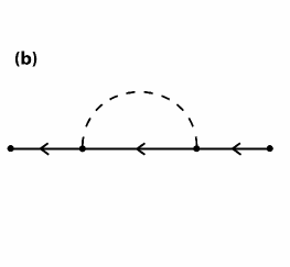
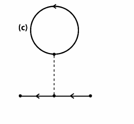
Figure 1: The calculated Feynman diagrams: (a) Is the unperturbed diagram, and (b) and (c) are first order linked diagrams. Diagram (c) contributes only to the annealed average.

6 Perturbation Theory And The Linked Cluster Theorem

Feynman diagrams [34] are an extremely useful tool which aid in the calculation of complicated functional derivatives by converting them into a diagrammatic form. These diagrams can be used to calculate the perturbative expansion of the correlation functions we require from $\overline{Z^{n}\left[\overline{\eta},\eta\right]}$. When constructing the possible Feynman diagrams of the disorder averaged correlation functions, we will discover that both linked and vacuum diagrams exist. Vacuum diagrams are those which contain two or more parts, while a linked diagram is completely connected. Examples of linked diagrams are shown in figures 1(b) and (c).

The linked cluster theorem demonstrates that when calculating correlation functions, vacuum diagrams cancel out and only the linked diagrams contribute. The numerator of the correlation functions is formed of a multiple of a sum of vacuum diagrams and a sum of linked diagrams while the denominator is a sum of vacuum diagrams only. The sums of vacuum diagrams therefore cancel, and we can write the correlation function as a sum over the linked diagrams.

The linked cluster theorem also shows that the replica method is exact in perturbation theory [1]. Taking the quenched limit is equivalent to eliminating diagrams containing fermion loops (as shown in figure 1 (c)). Fermion loops arise from the average introducing an interaction between different replicas. Prior to the average, a diagram with a loop is actually a vacuum diagram. In the quenched limit, these diagrams are no longer in the sum of linked diagrams, instead appearing in the sum of vacuum diagrams. Thus the quenched average leaves us a sum of linked diagrams without loops.

Since we will calculate both the quenched and annealed averages, we must find and calculate all linked diagrams.

7 Green Functions

Equation 4.1 shows that the correlation function we need for the average is $\overline{\langle d^{\dagger}(q)d(q)\rangle}$ which is found from equations 5.11 and 5.12 for the quenched an annealed averages respectively. To first order perturbation theory, the Feynman diagrams contributing to the correlation function are shown in figure 1. Using the standard rules for finite temperature many-body perturbation theory, we can calculate the contribution of each diagram (see, for example, [34, 35]).

For example, diagram figure 1 (b) gives us

$$2\frac{\Delta}{2}\int_{0}^{\beta}d\tau d\tau^{\prime}\int_{-\pi}^{\pi}\prod_{m=1}^{4}\left(\frac{dq_{m}}{2\pi}\right)\sum_{abcd}\delta_{ab}\delta_{cd}2\pi\delta\left(q_{1}-q_{2}+q_{3}-q_{4}\right)(e^{iq_{2}}+e^{-iq_{1}})$$ (7.1)

$$\times (e^{iq_{4}}+e^{-iq_{3}})2\pi\delta\left(q_{\beta}-q_{3}\right)\mathcal{G}\left(\tau_{\beta}-\tau^{\prime},q_{\beta}\right)\delta_{\beta c}2\pi\delta\left(q_{4}-q_{1}\right)$$

$$\times \mathcal{G}\left(\tau^{\prime}-\tau,q_{4}\right)\delta_{ad}2\pi\delta\left(q_{2}-q_{\alpha}\right)\mathcal{G}\left(\tau-\tau_{\alpha},q_{2}\right)\delta_{b\alpha},$$

where $\mathcal{G}\left(\tau-\tau^{\prime},q\right)$ was defined in equation 5.7. The multiple of $2$ at the beginning indicates there are two topologically distinct ways in which we can make this diagram. In order to recover the appropriate correlation function, we set $q_{\beta}=q_{\alpha}$ and $\tau_{\beta}=\tau_{\alpha}$, and perform the analytically possible integrals. This leaves us with the $\cos^{2}[(p+q)/2]$ term in $\overline{G}_{R}$ below.

We find that the expansion of the correlation function gives

$$\overline{G}_{R} = \int_{-\pi}^{\pi}\frac{dq}{2\pi}\cos\left(qR\right)\Bigg{\{}\left[1-2k(q)\right]$$

$$+ 8\Delta\int_{-\pi}^{\pi}\frac{dp}{2\pi}\left[\cos^{2}\left(\frac{p+q}{2}\right)\left\{\frac{k(q)-k(p)}{\left[\varepsilon(p)-\varepsilon(q)\right]^{2}}-\frac{\beta k(q)[1-k(q)]}{\varepsilon(p)-\varepsilon(q)}\right\}\right.$$

$$- \beta^{2}n^{2}\cos p\cos qk(p)\left[1-k(q)\right]k(q)\Bigg{]}\Bigg{\}}$$

As discussed previously, for the quenched average, $n\rightarrow 0$ so the final term in the above equation is zero while for the annealed average, $n=1$.

If we take the limit $\beta\rightarrow\infty$, we gain the zero temperature equivalent:

$$\overline{G}_{R} = \frac{1}{R\pi}\left[(1+e^{i\pi R})\sin\left(\frac{\pi R}{2}\right)-2\sin\left(\alpha R\right)\right]$$ (7.3)

$$+ 4\Delta\int_{0}^{\pi/2}\frac{dp}{\pi}\int_{0}^{\alpha}\frac{dq}{\pi}\left(\frac{\left[1+\cos p\cos q\right]\left[\cos(qR)-\cos(pR)\right]}{\left[\varepsilon(p)-\varepsilon(q)\right]^{2}}\right.$$

$$+ \left.\frac{\left[1-\cos p\cos q\right]\left[\cos(qR)-e^{i\pi R}\cos(pR)\right]}{\left[\nu(p)-\varepsilon(q)\right]^{2}}\right)$$

where $\nu(x)=2(B+J\cos x)$ and

$$\alpha=\left\{\begin{array}[]{lcl}\cos^{-1}(B/J)&\mbox{for}&B<J\\ 0&\mbox{for}&B\geq J.\end{array}\right.$$

We note that the quenched and annealed averages are identical in the $T=0$ case.

We are now in a position to calculate the concurrence as described in previous sections. In terms of $\overline{G}_{R}$, the nearest neighbour concurrence ($R=1$) is

$$\overline{\mathcal{C}}_{1}=\left\{0,\left|\overline{G}_{1}\right|-\frac{1}{2}\sqrt{\left(1+\overline{G}_{0}^{2}-\overline{G}_{1}^{2}\right)^{2}-4\overline{G}_{0}^{2}}\right\},$$ (7.4)

and the next nearest neighbour concurrence ($R=2$) is

$$\overline{\mathcal{C}}_{2}=\left\{0,\left|\overline{G}_{1}^{2}-\overline{G}_{2}\overline{G}_{0}\right|-\frac{1}{2}\sqrt{\left(1+\overline{G}_{0}^{2}-\overline{G}_{2}^{2}\right)^{2}-4\overline{G}_{0}^{2}}\right\}.$$ (7.5)

Then using equations 7.1 (and 7.3 for zero temperature), we can find the quenched and annealed averages of the concurrence.

We also plan to briefly discuss the single-site entanglement entropy, $\overline{S}(\rho_{l})=-\{(1+\overline{G}_{0})\log_{2}[(1+\overline{G}_{0})/2]+(1-\overline{G}_{0})\log_{2}[(1-\overline{G}_{0})/2]\}/2$ which measures entanglement at zero temperature between a single site and the rest of the spin chain. In addition we discuss the two-site entanglement entropy, $\overline{S}(\rho_{l,l+1})=-a\log a-c\log c-d\log[(b+d)/(b-d)]-b\log(b^{2}-d^{2})$ where $a=[(1+\overline{G}_{0})^{2}-\overline{G}_{1}^{2}]/4$, $b=(1-\overline{G}_{0}^{2}+\overline{G}_{1}^{2})/4$, $c=[(1-\overline{G}_{0})^{2}-\overline{G}_{1}^{2}]/4$ and $d=-\overline{G}_{1}/2$, which again can be used at zero temperature, and measures the entanglement between the two sites and the rest of the chain.

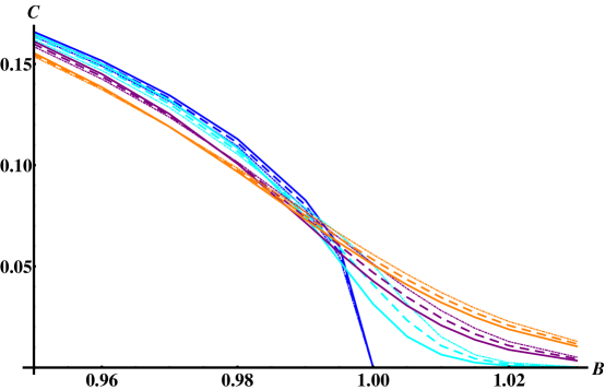
Figure 2: Quenched nearest neighbour concurrence around the quantum critical point. The solid lines are no disorder, the longer dashes $\Delta=0.0005$ and the short dashes $\Delta=0.001$. The blue lines are $T=0$, the cyan lines $T=0.01$, the purple lines $T=0.02$ and the orange lines $T=0.03$.

8 Disorder Averaged Concurrence

We have restricted the plots to be close to the quantum critical point (QCP) which for this system occurs at $B=J$ since this is the region where the effect of the disorder is the most interesting.

Figure 2 demonstrates how the quenched nearest neighbour concurrence behaves as the magnetic field varies for different values of temperature and disorder. We find that at zero temperature, increasing $\Delta$ always decreases the concurrence, and no new entanglement is created above the QCP. For finite temperatures, there is a crossover point of the magnetic field, $B_{c}$, below which increasing $\Delta$ decreases concurrence, and above which, increasing $\Delta$ increases concurrence. As the temperature increases, $B_{c}$ generally decreases while the amount that $\Delta$ increases the concurrence above $B_{c}$ decreases.

For the annealed nearest neighbour concurrence, shown in figure 3, we find a similar pattern of behaviour. However, $B_{c}$ in this case is much lower than for the quenched average. Both the quenched and annealed next nearest neighbour concurrence, shown in figures 4 and 5 respectively again give similar results, but with lower values for the concurrence overall.

A possible reason for the behaviour described above could be that the disorder has a similar effect on entanglement to the temperature. Both have the effect of mixing energy levels allowing for the possibility of creating entanglement above the QCP. However, at higher temperatures and lower magnetic field, the likely effect of more mixing is to decrease entanglement.

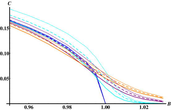
Figure 3: Annealed nearest neighbour concurrence around the quantum critical point. The solid lines are no disorder, the longer dashes $\Delta=0.0005$ and the short dashes $\Delta=0.001$. The blue lines are $T=0$, the cyan lines $T=0.01$, the purple lines $T=0.02$ and the orange lines $T=0.03$.

A puzzling feature of these results is that disorder does not increase the concurrence above the QCP at zero temperature as we would expect following the reasoning in the argument above. We expect that we would need to calculate the perturbation series to a higher order to see this behaviour. Alternatively, perhaps the value of $\Delta$ simply needs to be larger than perturbation theory is valid for to show this.

We have also calculated the correlation functions for a random magnetic field, when $H_{1}(b_{l})=\sum_{l}b_{l}\sigma_{l}^{z}$. Again we find the same behaviour for the concurrence, with a crossover point, $B_{c}$, close to the QCP for the quenched average and lower for the annealed average, and zero concurrence at $T=0$ for $B\geq J$ for both nearest and next nearest neighbour concurrence. Close to the QCP, increasing $\Delta$ for $b_{l}$, increases the concurrence more than for $j_{l}$ for both nearest and next nearest neighbour entanglement.

In addition to the concurrence we have considered the single and two site entanglement entropy. Since $\overline{G}_{0}=G_{0}$ at zero temperature, disorder doesn’t affect the single-site entanglement entropy in the regime we are able to apply perturbation theory in. This is the case for whether the randomness is in $j_{l}$ or $b_{l}$.

Interestingly, the two-site entanglement entropy actually increases with disorder for both $j_{l}$ and $b_{l}$ for all values of $B$. Increasing $\Delta$ increases the amount of entanglement by a larger amount the closer $B$ gets to $J$ for each. The random magnetic field, $b_{l}$, has a greater effect on the entanglement that $j_{l}$; increasing $\Delta$ by the same amount increases the entanglement entropy more for $b_{l}$ than for $j_{l}$.

We compare our results to [11] which uses sampling to look at an $XX$ spin chain in a random magnetic field. They consider concurrence at zero temperature, and the random field taken from a Gaussian distribution as well as a Lorentzian distribution. They find that increasing the disorder below the QCP decreases the nearest neighbour concurrence, while above the QCP, increasing disorder increases the concurrence. While our results for zero temperature agree with this behaviour below the QCP, above $B=J$, concurrence remains zero for us. However, we consider weak disorder while the lowest disorder [11] calculates is an order of magnitude larger than ours. It is possible that calculating the perturbative expansion to higher order would allow us to observe this behaviour.

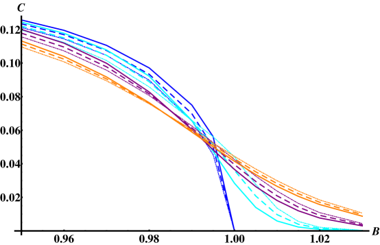
Figure 4: Quenched next nearest neighbour concurrence around the quantum critical point. The solid lines are no disorder, the longer dashes $\Delta=0.0005$ and the short dashes $\Delta=0.001$. The blue lines are $T=0$, the cyan lines $T=0.01$, the purple lines $T=0.02$ and the orange lines $T=0.03$.

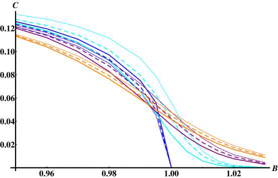
Figure 5: Annealed next nearest neighbour concurrence around the quantum critical point. The solid lines are no disorder, the longer dashes $\Delta=0.0005$ and the short dashes $\Delta=0.001$. The blue lines are $T=0$, the cyan lines $T=0.01$, the purple lines $T=0.02$ and the orange lines $T=0.03$.

9 Conclusions

We have found that for weak disorder, concurrence, the entanglement between qubit pairs, in general decreases with increasing quenched disorder. At non-zero temperatures, close to the QCP, disorder instead acts to increase entanglement. In the case of two-site entanglement entropy, (remembering this is a measure of entanglement only at zero temperature), the entanglement between two sites and the remainder of the spin chain, increasing the disorder increases entanglement.

Our results demonstrate that disorder is not necessarily detrimental to entanglement and thus to schemes which use it as a resource. This is, however, dependent on which entanglement measure is appropriate and the parameter regime we consider.

We can use the perturbation theory method to find the disorder averaged concurrence for other systems. However, if the system cannot be expressed as a free fermion (non-interacting) model, the number of disorder averaged correlation functions required would be increased since Wick’s theorem could no longer be applied. For example, we would no longer have $\overline{\langle\sigma_{l}^{z}\sigma_{l+1}^{z}\rangle}=\overline{G}_{0}^{2}-\overline{G}_{R}^{2}$, and would instead need to calculate a four-point correlation function since $\overline{\langle\sigma_{l}^{z}\sigma_{l+1}^{z}\rangle}=2\overline{G}_{0}-1+4\overline{\langle a_{l}^{\dagger}a_{l}a_{l+R}^{\dagger}a_{l+R}\rangle}$.

One strength of our paper is that we consider finite temperature as well as zero temperature entanglement. Since we use perturbative methods, our work has the propensity to be extended in many directions. For example, higher order calculations and application of the Dyson equation would be useful. In particular, perturbation theory allows for the consideration of time dependent non-equilibrium disorder averaged measures of entanglement using techniques such as the Keldysh formalism. This would be interesting since it would show how disorder affects the finite temperature entanglement of a system as it evolves over time.

References

References

• [1] Altland A and Simons B 2006 Condensed matter field theory (Cambridge University Press)
• [2] Abrikosov A A, Gor’kov L P and Dzyaloshinskii I. Ye. 1992 Methods of Quantum Field Theory in Statistical Physics (Pergamon Press)
• [3] De Dominicis C and Giardina I 2006 Random Fields and Spin Glasses: A Field Theory Approach (Cambridge University Press)
• [4] Dasgupta C and Ma S 1980 Phys. Rev. B 22 1305
• [5] Fisher D S 1994 Phys. Rev. B 50 3799
• [6] Amico L, Fazio R, Osterloh A and Vedral V 2008, Rev. Mod. Phys. 80 517
• [7] Refael G and Moore J E 2004 Phys. Rev. Lett. 93, 260602
• [8] Laflorencie N 2005 Phys. Rev. B 72, 140408(R)
• [9] Santachiara R 2006 J. Stat. Mech. L06002
• [10] De Chiara G, Montangero S, Calabrese P and Fazio R 2006 J. Stat. Mech. P03001
• [11] Fujinaga M and Hatano N 2007 J. Phys. Soc. Jpn. 76, 094001
• [12] Binosi D, De Chiara G, Montangero S and Recati A 2007 Phys. Rev. B, 76, 140405(R)
• [13] Refael G and Moore J E 2007 Phys. Rev. B 76, 024419
• [14] Hoyos J A and Rigolin G 2006 Phys. Rev. A 74 062324
• [15] Hide J, Son W and Vedral V 2009 Phys. Rev. Lett. 102 100503
• [16] Hide J and Vedral V 2010 Physica E 42, 359
• [17] Bose S 2003 Phys. Rev. Lett. 91 207901
• [18] Bose S 2007 Contemp. Phys. 48 13
• [19] Bayat A and Karimipour V 2005 Phys. Rev. A 71 042330
• [20] Bayat A and Bose S 2010 Adv. Math. Phys. 2010 1
• [21] Wang X, Bayat A, Schirmer S G and Bose S 2010 Phys. Rev. A 81 032312
• [22] Burgarth D and Bose S 2005 New J. Phys. 7 135
• [23] Burrell C K and Osborne T J 2007 Phys. Rev. Lett. 99 167201
• [24] Burrell C K, Eisert J and Osborne T J 2009 Phys Rev A 80 052319
• [25] Allcock J and Linden N 2009 Phys. Rev. Lett. 102 110501
• [26] Petrosyan D, Nikolopoulos G M and Lambropoulos P 2010 Phys. Rev. A 81 042307
• [27] Wells B O, Lee Y S, Kastner M A, Christianson R J, Birgeneau R J, Yamada K, Endoh Y and Shirane G 1997 Science 277 1067
• [28] Anicich P G O and Grinberg H 2002 Int. J. Quant. Chem. 90 1562
• [29] Wootters W K 1998 Phys. Rev. Lett. 80 2245
• [30] Hill S and Wootters W K 1997 Phys. Rev. Lett. 78 5022
• [31] Bennett C H, Bernstein H J, Popescu S and Schumacher B 1996 Phys. Rev. A 53 2046
• [32] Barouch E and McCoy B M 1971 Phys. Rev. A 3 786
• [33] Le Bellac M 2000 Thermal Field Theory (Cambridge University Press)
• [34] Mattuck R D 2006 A Guide to Feynman Diagrams in the Many-body Problem (Dover Publications)
• [35] Negele J W and Orland H 1998 Quantum many-particle systems (Westview Press)