Ubercalibration of the Deep Lens Survey

Abstract

We describe the internal photometric calibration of the Deep Lens Survey, which consists of five widely separated fields observed by two different observatories. Adopting the global linear least-squares (“ubercal”) approach developed for the Sloan Digital Sky Survey (SDSS), we derive flatfield corrections for all observing runs, which indicate that the original sky flats were nonuniform by up to 0.13 mag peak to valley in ${z}$ band, and by up to half that amount in BVR. We show that application of these corrections reduces spatial nonuniformities in corrected exposures to the 0.01-0.02 mag level. We conclude with some lessons learned in applying ubercal to a survey structured very differently from SDSS, with isolated fields, multiple observatories, and shift-and-stare rather than drift-scan imaging. Although the size of the error caused by using sky or dome flats is instrument- and wavelength-dependent, users of wide-field cameras should not assume that it is small. Pipeline developers should facilitate routine application of this procedure, and surveys should include it in their plans from the outset.

1. Introduction

As CCD camera fields of view have become dramatically larger in the past decade, ensuring uniform photometry has become more challenging. Traditionally, it is assumed that the camera can be uniformly illuminated, by sky emission or by an illuminated screen, and dividing by the response of each pixel to this illumination is all that is necessary to make images internally consistent. But the sensor may not be uniformly illuminated due to vignetting or to nonuniform sources of illumination such as scattered light, moonlight, or ghosting.

These problems are exacerbated when the field of view is large. For small fields of view, a reasonable workaround for nonuniform illumination is to observe a given star with a grid of pointings, so that spatially-varying photometry can be directly identified and modeled out. This is impractical for very large cameras, where the observation and readout times would be prohibitive. However, Padhmanabhan et al. (2008, hereafter P08) presented a nearly-equivalent solution involving multiple stars. In any set of overlapping exposures or drift scans, some stars are multiply observed, in different parts of the camera, and these observations can be used to constrain a model of the spatial variation of the camera response. This technique, widely referred to as ubercal, analyzes the survey data per se, and does not require additional calibration data. This neatly separates the problems of internal and external calibration.

As more and bigger imaging surveys come online, ubercal is sure to be an important tool. P08 applied it to a drift-scan survey, the Sloan Digital Sky Survey (SDSS). We apply it here to the Deep Lens Survey (DLS) which, like the vast majority of imaging surveys, is a shift-and-stare survey. The DLS has some other peculiarities, such as widely separated fields and multiple observatories, that make it an informative example for the application of this technique. In §2 we describe the DLS and the corresponding structure of the ubercal model; in §3 we describe the fitting process; in §4 we show the results and examine their robustness; in §5 we report the impact on survey photometry accuracy; and we present conclusions in §6.

2. Ubercal formalism for the DLS

The basic idea of ubercal is to write down a model describing the observing process (true magnitudes are offset by a zeropoint, an airmass term, and a “flatfield” term describing the spatial variation of the camera response), and constrain the model parameters using the measured instrumental magnitudes. Before writing a specific model for the DLS, we first describe the structure of the DLS.

2.1. Structure of the DLS

The DLS consists of five well-separated 2${}^{\circ}\times 2^{\circ}$ fields (Table 1). The northern fields (F1 and F2) were observed using the Kitt Peak Mayall 4-m telescope and Mosaic prime-focus imager (Muller et al. 1998). The southern fields (F3 through F5) were observed with a similar setup at the Cerro Tololo Blanco 4-m telescope. Each Mosaic imager consists of a 4$\times$2 array of three-edge-buttable 2k$\times$4k CCDs, providing a 35${}^{\prime}\,$ field of view with 0.26${}^{\prime\prime}\,$ pixels and minimal gaps between the devices. Each DLS field is divided into a 3$\times$3 grid of 40${}^{\prime}\,$$\times$ 40${}^{\prime}\,$ subfields. These subfields are slightly larger than the Mosaic field of view, but are synthesised with dithers of up to 800 pixels (208${}^{\prime\prime}\,$). In some cases, dithers were much larger. For example, CCD 3 was dead during two Cerro Tololo runs, and we dithered by an entire chip width (8.5${}^{\prime}\,$). In a small number of exposures, telescope pointing errors resulted in very large dithers and/or odd pointing centers, further tying the subfields together.

Table 1DLS field centers (J2000) and mean extinctions from Schlegel, Finkbeiner & Davis (1998).

Field	RA	DEC	l,b	E(B-V)
F1	00:53:25.3	+12:33:55	125,-50	0.06
F2	09:18:00	+30:00:00	197, 44	0.02
F3	05:20:00	-49:00:00	255,-35	0.02
F4	10:52:00	-05:00:00	257,47	0.025
F5	13:55:00	-10:00:00	328,49	0.05

The DLS was observed in four filters, BVR${z}$. $R$ was observed when the seeing FWHM was $<0.9$${}^{\prime\prime}\,$; if the seeing was worse, the choice of filters was dictated by moon phase, airmass, and past progress in other filters. Thus, most nights contain images in multiple filters, but few nights contain images in all four filters. There were 25 observing runs of 2-6 nights each. On a few runs, southern fields (F4 at declination -5^∘ and F5 at -11^∘) were observed from Kitt Peak. A northern field (F1 at declination +12^∘) was observed on only one Cerro Tololo run, on a nonphotometric night. At both sites, equatorial standard star fields (Landolt 1992, Smith et al. 2002) were observed on photometric nights. More details about the DLS survey design and image processing can be found in Wittman et al. (2002) and Wittman et al. (2006) respectively. A paper describing the final data release details (Wittman et al., in preparation) is forthcoming.

2.2. Photometric model

We adopt the following model for the instrumental magnitudes measured through a given filter:

$$m_{instr}=m_{true}^{(s)}+z^{(r)}+k^{(n)}A+f^{(r,c)}(x,y)$$ (1)

where $z$ is a run-dependent zeropoint, $A$ is the airmass of the observation, $k$ is the extinction per unit airmass, $f$ is the flatfield function, and superscripts indicate indexing by star $(s)$, run $(r)$, night $(n)$, and CCD $(c)$ identification numbers. Filter superscripts are not explicitly written here because the fitting procedure is carried out totally independently in each filter.

We choose $f$ to be a second-order polynomial in the CCD coordinates $x$ and $y$, with an $xy$ cross-term making a total of 6 parameters per CCD. There is no requirement that the flatfield be continuous across CCD boundaries. The primary motivation for allowing discontinuities is that sky flats have already been applied to the data, so we are really modeling systematic errors in the sky flat process, which may include discontinuous jumps at the CCD boundaries. The flatfield magnitude offset at the center of the first CCD is fixed at zero to remove the degeneracy with overall throughput parameters such as the zeropoint. This leaves 47 flatfield parameters to constrain for each run (eight CCDs times six polynomial parameters, minus one fixed offset). Each run has its own flatfield model, because sky flats were derived and applied on a per-run basis.

Each run also has its own zeropoint, so that the model can track changes in non-atmosphere-related observatory throughput such as might occur when the telescope optics are recoated. Changes in CCD gain would also be absorbed into this factor.

Airmass terms are, in principle, fit for each night. In practice, many nights were not photometric, and thus cannot be fit this way. On these nights, each image receives its own airmass term. This conceptually the same as receiving its own zeropoint, but happens to be simpler to implement in our code. A few images were taken with nonstandard exposure times. For fitting purposes, we converted the instrumental magnitudes from these exposures to the instrumental magnitudes that would have been observed had the standard exposure time been used.

We choose not to model any time variation of the airmass term. P08 suggest a time term of 1 mmag per unit airmass per hour, based on data from the SDSS photometric calibration telescope. The sign is such that the atmosphere grows more clear as the night goes on. We have no information on similar trends at Cerro Tololo and Kitt Peak. DLS differs from SDSS in being able to use only one filter at a time, so that time baselines in a given filter tend to be much shorter. Over a three-hour time baseline, a change of 1 mmag per unit airmass per hour is quite small. Furthermore, because DLS has fixed fields rather than a drift-scan strategy, airmass is often a monotonic function of time in a given filter on a given night, in which case much of the time variation (if it even exists) can be absorbed into the airmass term. Therefore, we do not include time variation as part of the model. This is further justified by the general absence of time trends in the residuals.

2.3. Spatiotemporal degeneracy

Our primary motivation for this work was to derive the flatfield corrections, because the DLS photometry had been showing spatial dependence. Recall that each subfield was imaged 20 times in each filter, with $\sim 5$${}^{\prime}\,$dithers providing some overlap between adjacent subfields. Intuitively, one might think that this large number of dithers would be sufficient to constrain the flatfield corrections by itself. However, there is an astonishing degeneracy between spatial and temporal variations, as follows.

Consider an imaging device with a sensitivity variation $f(x,y)=ax+by$ (in magnitudes here for convenience) and a time-varying zeropoint $z(t)$. For now we will not think of $z(t)$ as a function, but just as a collection of zeropoints at the times $t_{i}$ when various exposures were taken. So a star at position $x,y$ will have instrumental magnitude

$$m_{i}=m_{true}+ax+by+z(t_{i})$$ (2)

Now consider a set of exposures with dither offsets $x_{i},y_{i}$. The difference between instrumental magnitudes of a given star on the $i$th and $j$th exposures is

$$m_{i}-m_{j}=a(x_{i}-x_{j})+b(y_{i}-y_{j})+z(t_{i})-z(t_{j})$$ (3)

This quantity is identical for all stars and galaxies, because they all experience the same spatial shift.

Now consider an alternative model where the flatfield slopes are quite different:

$$m_{i}=m_{true}+(a+\lambda_{1})x+(b+\lambda_{2})y+z(t_{i})-\lambda_{1}x_{i}-\lambda_{2}y_{i}$$ (4)

with $\lambda_{1}$ and $\lambda_{2}$ being arbitrary numbers making it clear that this model is different from the previous model. Recall that x and y are the star’s position on the detector, while $x_{j}$ and $y_{j}$ are the dither shifts, so the last two terms affect the entire exposure, effectively changing its zeropoint. Now the difference between exposures is

$$m_{i}-m_{j} =(a+\lambda_{1})(x_{i}-x_{j})+(b+\lambda_{2})(y_{i}-y_{j})$$

$$+z(t_{i})-z(t_{j})-\lambda_{1}(x_{i}-x_{j})-\lambda_{2}(y_{i}-y_{j})$$

$$=a(x_{i}-x_{j})+b(y_{i}-y_{j})+z(t_{i})-z(t_{j})$$ (5)

Equations 3 and 5 are the same, demonstrating that the observed magnitude difference is identical in these two cases, despite their very different implications for the flatness of the detector sensitivity, and therefore for all the photometry derived therefrom. This is a degeneracy.

Note that the degeneracy parameters $\lambda_{1}$ and $\lambda_{2}$ do not depend on the position of the star on the detector, only on the dither offset $x_{i}-x_{j},y_{i}-y_{j}$. Therefore, the density and spatial distribution of stars is irrelevant. Furthermore, the $\lambda_{i}$ depend only on the $i$th exposure’s dither offset, not on any properties of the other exposures. Therefore, the number and spatial distribution of dithers is irrelevant. This is a true degeneracy as long as the zeropoints have freedom to soak up any effect of the flatfield slope. But with observations in photometric conditions, we can put a strong prior on $z(t_{i})-z(t_{j})$, thus constraining the linear flatfield terms $a$ and $b$ to similar precision in units of the dither size. Surveys with substantial fractions of nonphotometric time should be aware of this issue. For example, they should ensure that the nonphotometric time is not overly concentrated in any one filter, lest it become impossible to solve for the flatfield corrections in that filter.

This degeneracy is grasped much more intuitively and directly by considering a technique used for small cameras, dithering a given star around the field of view to directly measure the flatness of the photometry. Clearly, that procedure would work only if done quickly enough to eliminate the possibility of changes in throughput due to anything other than star position. Similarly, ubercal requires a strong temporal or airmass-based constraint on each exposure’s throughput.

One might think that another way to fix the degeneracy would be to rotate the CCD. Although this does constrain the gradient, there are still rotational modes which are degenerate with the time behavior. We have confirmed this with simulations.

If $f(x,y)$ contains higher-order polynomial terms, these are not degenerate. For example, the signature of a 2nd-order term might be stars on the left side of the CCD getting brighter and stars on the right side getting fainter after a small shift to the left, and vice versa for a small shift to the right. This cannot be mimicked by a zeropoint change. However, the linear terms are independent of the higher-order terms and thus will remain unconstrained even in the presence of the higher-order terms.

2.4. Other degeneracies

There are other degeneracies modelers should be aware of. Most of these were recognised by P08, but are worth mentioning here in the context of a very differently structured survey.

Absolute calibration degeneracy. The bulk of the fit parameters are the “true” magnitudes of the stars. Of course, these are not true magnitudes in an absolutely calibrated sense. There is a degeneracy in which uniform increase in true magnitudes can be compensated by a uniform decrease in run zeropoints. Fixing this degeneracy is precisely the problem of external calibration, which we do not address here.

Relative calibration degeneracy for isolated fields. The true magnitudes in one field are fixed relative to the true magnitudes in another field only if both fields were observed from the same observatory on the same photometric night. Non-photometric cross-observations do not help because per-image zeropoints are free to absorb any offset in the true magnitudes of one field relative to the other field. Almost every photometric night of DLS observations touched multiple fields, so most fields are well tied together. However, there is a natural north-south split with few photometric cross-observations. The B, V and ${z}$ observations contain at least one photometric night with cross-hemisphere observations. However, in R there are none. This could be fixed with external calibrations from the standard star fields. However, in the spirit of ubercal, we make use of the fact that both observatories often observed the same equatorial standard star fields, in particular SA 98 and SA 101 (Landolt 1992). Therefore, we included SA 98 and SA 101 data in the ubercal fit, not to provide absolute calibration, but to strengthen the ties between north and south. (One could make ubercal perform both of these functions by fixing $m_{true}$ for the Landolt (1992) stars rather than considering them nuisance parameters. However, this would require all ubercal photometry to be measured within a large (14${}^{\prime\prime}\,$ diameter) aperture to be consistent with Landolt (1992). Therefore, the absolute calibration is better done outside the ubercal framework.)

Airmass/time degeneracy. On many DLS nights, there is a monotonic relationship between airmass and time for some of the filters, because a given filter was used for only a few hours before or after a field transited. Thus, a time-dependent term would be degenerate with an airmass term. This degeneracy does not prevent one from producing internally consistent photometry, but it does severely hamper physical interpretation of the fit parameters. Consider a time-dependent airmass coefficient of the form $k+k_{1}t$. With $k_{1}$ fixed at zero, the size of $k$ is an indicator of the clarity of the night, and very large or very small $k$ indicates some problem with the data (most likely clouds if $k$ is very large, for example). With $k_{1}$ free, we find that the data will be slightly better fit, but the time/airmass degeneracy will probably drive $k$ and $k_{1}$ to nonphysical values. We therefore choose not to fit for $k_{1}$.

3. Fitting

The procedures described below were carried out independently in each filter, unless otherwise noted.

3.1. Input data

We ran SExtractor (Bertin & Arnouts 1996) to produce a catalogue for each CCD of each exposure, and then matched the catalogues in RA and DEC to produce a master catalogue for each widely separated field. (This is an exception to the per-filter rule; all images in a given field were matched to ensure consistent astrometry across filters.) Because the eventual goal is to stack the images onto a grid with uniform pixel size, we added master $x,y$ columns corresponding to the desired output grid. We also assigned a unique identification number to each object in the master catalogues. We then matched each CCD catalogue to the master catalogue and fit for polynomial coordinate transforms between CCD coordinates and uniform-grid coordinates. We corrected the photometry of each CCD catalogue by the Jacobian of the coordinate transform, to correct for the varying pixel size without resampling the pixels. See the DLS data release paper (Wittman et al., in preparation) for a more complete explanation of this correction. As noted above, in a few cases we also adjusted the magnitudes to the standard exposure time.

We then cleaned the catalogues. We rejected observations with SExtractor FLAGS$>$0, and cut on object peak intensity (SExtractor’s FLUX_MAX output parameter). On this attribute, we imposed both a maximum (20% below saturation after taking into account the sky level which is not included in FLUX_MAX) and a filter-dependent minimum designed to prevent the catalogues from becoming extremely large. The minimum was set around 35$\sigma$ (for the peak pixel, not the entire detection) in ${z}$ band, and higher in the other bands. Roughly 100 objects per CCD pass these cuts, yielding roughly 800 objects per exposure and roughly 800,000 objects per filter. The time required to fit a catalogue of this size turned out to be surprisingly short (see §3.3), so that the catalogs could have been made more inclusive. However, some lower signal-to-noise ratio (S/N) cutoff will always be necessary, as low-S/N objects add limited constraining power while increasing the compute time linearly. We prefer a conservative S/N cut because SExtractor overstates the S/N by not accounting for sky modeling errors.

We used both stars and galaxies. P08 used only stars “to avoid subtleties of extended object photometry.” However, these subtleties are mostly due to the range of galaxy profiles and morphology. Because we are only concerned with relative photometry of the same galaxy appearing in different places on the sensor, galaxy photometry should be usable for this purpose. In tests, we found SExtractor’s MAG_AUTO (the magnitude within an aperture of size and shape determined by the object itself) to be relatively immune to seeing variations, so we used MAG_AUTO for the fit.

However, the stated uncertainties on MAG_AUTO are unrealistically small ($\sim$ 1 mmag) because they are based on photon noise. For bright objects, where photon noise is relatively small, measurement uncertainty is likely dominated by background modeling errors. At the bright end, we found a noise floor of $\sim$0.02 mag as determined by the rms differences between magnitudes measured for the same object on pairs of images closely matching in time, airmass, and detector position. This value is only a rough approximation, as it is certainly filter-dependent, and may decrease after taking flatfield corrections into account, but it is much more realistic than the nominal uncertainties, so we assign an uncertainty of 0.02 mag to each measurement. When interpreting the $\chi^{2}$ values from the fit, we must keep in mind the roughness of the approximation here.

The cleaned catalogue in any given filter contains 5-7$\times 10^{5}$ observations and 6-7$\times 10^{4}$ unique objects, depending on filter. The cleaned catalogue does not contain any objects observed only once. Thus it should not contain cosmic rays or asteroids, except where they happened to land on top of real objects. In §3.3 we describe how to reject those observations.

3.2. Photometricity of nights

Before using ubercal, our previous method of determining photometric offsets between exposures was by matching exposure catalogues against a master catalogue. These offsets, along with observing logs and standard star observations taken on nights thought to be photometric by the observers, gave us a good starting point for marking nights as photometric (and thus requiring a single $k^{(n)}$ parameter for the night) or nonphotometric (and thus requiring an exposure-specific magnitude offset). However, we found (as did P08) that ubercal itself was the best tool for picking up on subtle levels of cloud. Nonphotometric nights stood out as having many exposures with large mean residuals from the fit. When a night was identified as nonphotometric, the $k^{(n)}$ parameter for that night was removed from the model, one extinction parameter per exposure was inserted, and the fitting was restarted from scratch. The process was iterative, with ever-better overall fits highlighting ever more subtle photometricity variations. As described below, we found that even the best-fit nights have unmodeled variations, so that the cutoff between photometric and nonphotometric is somewhat arbitrary. We adopted a rule calling a night photometric if the vast majority of its exposures were modeled to within 0.02 mag.

Figure 1 illustrates the process of identifying nonphotometric nights. Each color in the figure represents a different night on one run (all in $B$ band). We rearrange Equation 1 to isolate the airmass part of the model:

$$m_{instr}-(m_{true}^{(s)}+z^{(r)}+f^{(r,c)}(x,y))=k^{(n)}A.$$ (5)

We then average the left-hand side over the hundreds of objects photometered in that exposure to obtain a single point for that exposure. These are the points plotted in the top panel of Figure 1. For one night (shown in black), the points cluster around a straight line. This is the airmass model on the right-hand side of Equation 5, which is also drawn on the figure. For two other nights (shown in blue and green), there is a huge variance in the upper panel. It appears that the telescope was pointed at relatively clear sky for part of each night (points lined up near the black line), but obviously cloudy sky for a substantial number of exposures (points well above 0.3 mag on the vertical axis). The conclusion is that those nights were not photometric, and therefore no airmass fit is drawn. Instead, each nonphotometric exposure is assigned a unique value of $kA$ in Equation 5, equal to the mean of the left-hand side of the equation. For the night which was fit with a single parameter, the residuals (as a function of airmass and of time) are shown in the lower two panels.

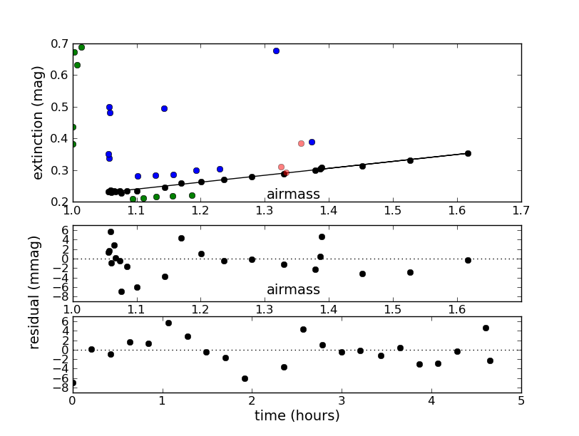
Figure 1.— Airmass fits and residuals for a run with one photometric and three nonphotometric nights in $B$ band. Each point represents one exposure and each night is a different color. The bottom panel shows the residuals from the fit (after averaging all objects in each exposure) as a function of time, and the middle panel shows the residuals as a function of airmass. The top panel shows the model and data relative to the run zeropoint, such that the lines should intercept zero magnitudes at zero airmass.

The night shown in red has only three exposures in this filter, so the evidence is not as strong as for the other nights, but variable cirrus may have been a factor. In cases like these, the presumption should be nonphotometric. The time and airmass baselines are short, so even if the data were photometric they would not provide strong additional constraints beyond their base nonphotometric value. We stress that even nonphotometric data help constrain the flatfields. The extinction due to clouds is unlikely to have spatial structure on the scale of the camera (35${}^{\prime}\,$), especially integrated over an exposure time of 10-15 minutes. Therefore, as long as other data in the survey (on other runs, perhaps) constrain the true magnitudes of the objects in the relevant areas of sky, the spatial variation of the photometry in the nonphotometric exposure does provide information about the flatfield. So in the context of a larger survey with sufficient photometric data, ubercal can solve for the flatfield even for a completely nonphotometric run.

It is instructive to examine the residuals on photometric nights (lower panels of Figure 1). The fit is good over a wide range of airmass and time. The worst residuals are 6-7 mmag, whereas the measurement uncertainty on each residual is about 1 mmag. The residuals are also structured in time, with a quasiperiodic variation of $\sim 2$ hours and a peak-to-valley amplitude of $\sim 10$ mmag. These data do not tell us whether this variation in extinction occurred in all directions, or only in the particular field being followed. It seems likely that a local variation such as a band of very thin cirrus would move across the field on faster timescales, and that on photometric nights the long DLS exposures are more sensitive to global variations. However, surveys with much shorter exposure times will not necessarily find spatial variations to be trivial, and may find a wider-field boresighted cirrus monitor to be a good investment.

To be declared photometric, a night had to have not only a good airmass fit, but a physically plausible airmass coefficient ($\sim$ 0.05, 0.08, 0.14, and 0.22 in ${z}$, $R$, $v$, and $B$ respectively). Figure 2 shows histograms of the best-fit nightly airmass terms in the four filters, for those nights which were considered photometric. To prevent overfitting, the model enforces a common zeropoint throughout a run. In other words, the fits for two nights on the same run must intersect at zero airmass. Although there are physical mechanisms which could change the zeropoint at zero airmass (recoating of the optics, for example), few of them are likely to operate on a night-to-night timescale. We could obtain fits with slightly smaller residuals by freeing this constraint, but there is little physical motivation for doing so.

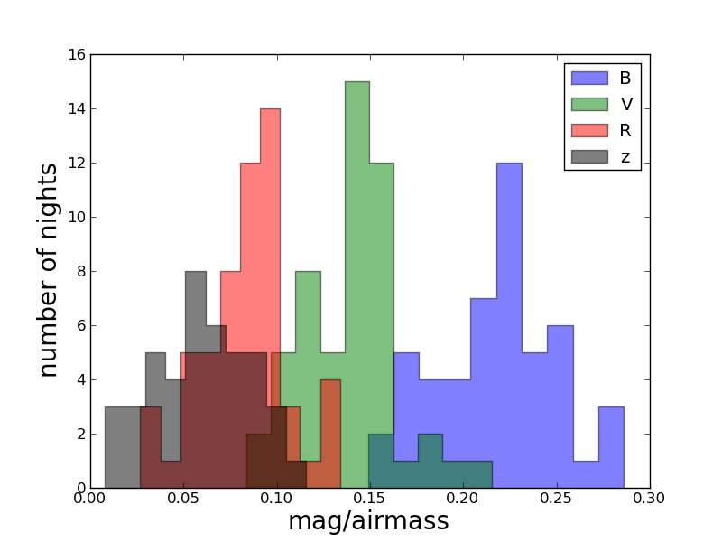
Figure 2.— Histograms of the best-fit nightly airmass terms, which cluster around the physically expected values in each filter. Nights which deviated greatly from these values were recognized as nonphotometric. Typically, such nights were poor fits anyway.

Two of the nights in Figure 1 are very obviously cloudy, but many cases were more borderline, with $\sim 0.1$ mag departures from the best airmass fit. Before definitively marking a night as nonphotometric, we investigated other possible explanations for a poor fit. In particular, because good flatfield solutions were our main goal, we investigated the possibility that a poor nightly fit could be caused by poorly fitting flatfields rather than nonphotometricity. We did this by checking for correlations between dither directions and residuals. For example, with respect to the first exposure of the five-exposure dither pattern, subsequent exposures were shifted 3.5${}^{\prime}\,$ shift to the northeast, 3.5${}^{\prime}\,$ shift to the southwest, 1.75${}^{\prime}\,$ shift to the northwest, and finally 1.75${}^{\prime}\,$ shift to the southeast. Thus, if a series of images fit poorly due to poor flatfield solutions, one would expect the residuals to reverse sign between the second and third, and/or the fourth and fifth, exposures of a dither pattern, and for the residuals to be largest on the second and third exposures. In fact, we never found this pattern, instead consistently finding the $\sim$2 hour quasiperiodic variation described above.

In cases of borderline photometricity we also looked at behavior in all filters on the same night. If the collective behavior seemed nonphotometric, we marked the night as nonphotometric. Once marked as nonphotometric for any reason, a night is considered nonphotometric in all filters.

A few images were flagged as outliers despite being on apparently photometric nights. About half of these had clearly identifiable causes, such as incorrect header information, or the last exposure of a night pushing too far into dawn and corrupting the input photometry. In the case of bad header information on a photometric night, the image was returned to the photometric list if the correct metadata (primarily airmass) could be reconstructed from observing logs. Otherwise, the image was considered as a singleton, receiving its own exactly fitted value of $kA$ just as if it were nonphotometric. The most interesting case was an exposure where apparently the guider jumped stars at some point, resulting in double images of everything (but one image several times fainter than the other). The fact that this was not flagged manually at the time of observation demonstrates the porosity of manual checks and the benefits of fitting all the survey data simultaneously.

3.3. Writing and running the code

The core fitting code was kindly provided by N. Padhmanabhan, written in C++ with a conjugate gradient optimiser based loosely on the one in Press et al. (1992). This is not the same code used in P08; it was written from scratch to assess the feasibility of ubercal for the Large Synoptic Survey Telescope (LSST, Abell et al. 2009), and only solved for per-image zeropoints. We modified the code for DLS, adding indexing by run, by night, and by CCD, and solving for polynomial flatfield solutions, airmass terms, and per-run zeropoint offsets. To avoid potential numerical instabilities, the polynomial coordinates are centered on each CCD and tracked in units of CCD widths rather than pixels. For convenience, the run zeropoints are referenced to the center of CCD 1 rather than to an average over the entire array.

The code takes only 6 minutes to converge on a standard desktop computer with $7\times 10^{5}$ data points and 6.5$\times 10^{4}$ parameters (mostly nuisance parameters, the true relative magnitudes of the objects). We declare convergence when an iteration yields a relative $\chi^{2}$ reduction of $10^{-9}$ or less. Because the total $\chi^{2}$ is about $\sim 6\times 10^{5}$ after convergence, this criterion corresponds to a $\chi^{2}$ reduction of much less than one per iteration, but due to the poorly defined photometric uncertainties the value of $\chi^{2}$ is less important than the fact that further iterations do not decrease it. This level of convergence takes about 3000 iterations. As an external check of convergence, we restart the fitter with the best parameters but no memory of the gradient, which forces the fitter to test a new direction in parameter space; the result was always consistent with the original solution.

We checked for images with large ($\gtrsim 0.05$ mag) rms scatter in the residuals, even if the mean residuals were acceptable. A few images with high sky levels due to approaching dawn were identified this way. These images appeared good to a casual inspection, e.g, the sky was not very close to saturation. Although they contributed relatively little information to the survey due to their high sky noise, the pre-ubercal judgment was to include them because they added something. However, the ubercal residuals were often highly non-Gaussian, hinting at sky-modeling problems or other subtle problems related to the bright sky. Therefore, the judgment changed: the small information contribution could be outweighed by other problems, and we decided to exclude these images from the survey.

As mentioned above, asteroids and cosmic rays can land on top of real objects and corrupt their photometry. For these and other reasons, we lightly clip the catalogue before fitting for the final solution. We clip at 6$\sigma$ plus the mean residual of the worst-fitting exposure (so that the worst-fitting exposure does not have many individual objects clipped simply due to some overall characteristic of the exposure). The rms residual is about 0.02 magnitudes (ranging from 0.015 in R to 0.025 in ${z}$), and the mean residual of the worst-fitting exposure ranges from 0.014 in V to 0.025 in B, thus setting a clip threshold of 0.10 to 0.17 magnitudes depending on the filter. Clipping removes the one outlying observation of an object, rather than all observations of that object. Manual inspection of some of the clipped observations confirmed that the causes were generally identifiable as cosmic-ray hits, proximity to an unmasked bad pixel or bleed, foreground asteroid, etc.

After clipping, the reduced $\chi^{2}$ is about unity. However, the value of $\chi^{2}$ is not a rigorous indication of goodness-of-fit because we manually set the instrumental magnitude uncertainties to 0.02 mag in the absence of realistic uncertainty estimates from SExtractor. The reduced $\chi^{2}$ ranges from 0.56 in $R$ to 1.65 in ${z}$ because the $R$ photometry is more precise than 0.02 mag ($R$ being the deepest filter and the one with the best seeing) and the ${z}$ photometry is less precise (due to the large sky noise). Thus the $\chi^{2}$ values indicate that the fits are plausibly good, but we base our judgment of the fits mostly on other considerations such as inspection of all the airmass plots and (as described below) physical plausibility of the solutions, closed-loop correction tests, and robustness against varying preparation of the input photometry.

4. Results

There are three main types of output: the nightly airmass terms, the run zero points, and the spatial sensitivity functions (“flatfields” for short). We show some examples of each and offer physical interpretations.

4.1. Airmass Terms

We have discussed the airmass fits already, because they are crucial to the iterative process of marking nights as nonphotometric and converging on a final fit. We therefore focus here on some examples which are atypical but which provide insight into the process.

Figure 3 shows the airmass fits for the January 2001 CTIO run in $R$ band. Three nights (shown in green, red, and blue) were well fit by a common run zeropoint plus nightly airmass terms. In other words, the fitted lines all converge to a point (the run zeropoint) at zero airmass. The first night (shown in black) has similar airmass slope but is offset by about 0.15 mag, i.e. it could never converge at the common run zeropoint. Put simply, exposures taken on this night contain about 15% greater flux at any given airmass. Possible causes fall into several categories:

1. the camera collected 15% more photons from each source on that night. There is no plausible physical scenario enabling this. If the other nights on the run were photometric with airmass terms $\sim$0.07, then even complete removal of the atmosphere would not suffice to increase throughput by this much.

2. the CCD amplifier gain differed by 15% on that night. This is unexpected, but not as implausible as the first scenario.

3. the data were changed after acquisition, for example, by multiplying all images from this night by 1.15, or applying a different flatfield than the other nights. There is no evidence in the image headers for this.

4. the photometry procedure is not robust, for example being seeing-dependent. However, the seeing on this night is not very different from the other nights on this run, and other runs with much larger seeing variations do not show this behavior.

5. exposure times were uniformly 15% longer on this night. This is implausible given the headers and observing logs.

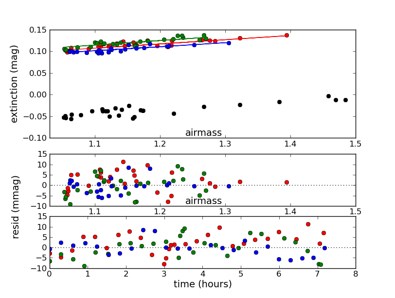
Figure 3.— Airmass fits for the January 2001 CTIO run in R band. Three nights (shown in green, red, and blue) were well fit by a common run zeropoint plus nightly airmass terms. One night (shown in black) has a magnitude offset which is too large and too airmass-independent to be an atmospheric variation. This kind of change could be caused by a change in overall scaling factor such as CCD gain.

Only $R$ data were taken on this night, so behavior in the other wavelengths, our cross-check of first resort, cannot be checked. Two other nights show similar behavior, but at a lower (4-5%) level. One of those nights contains observations in only one band, but the other contains observations in three bands, and all three bands are consistent. Because different bands are reduced totally independently, this makes it very unlikely that a data processing misstep is responsible, and more likely that a gain change is responsible. Whatever the cause, the practical impact is that these nights cannot be fit with the usual model of nightly airmass term and overall run zeropoint. In principle, they could be fit with a nightly airmass term plus nightly zeropoint, but for convenience we simply fit them with per-exposure zeropoints as if they were nonphotometric.

In Figure 4, we show a second example of unexpected behavior of the airmass fits. The night shown in green is best fit by a negative airmass term. This is completely unphysical, so the natural conclusion is that the night had varying amounts of clouds which happened to anticorrelate with the airmass. However, if that night had clouds, then the other nights on the run had even more clouds, which also implausibly conspired to yield airmass fits with small residuals. There is no indication of this in the observing logs, nor in the best-fit run zeropoint (which does not suggest overall extinction greater than other runs), nor in the other filters observed on these nights. A second hypothesis might be that the fit is forcing the night shown in green into unnatural behavior because all the best-fit lines must converge at zero airmass. But freeing that night to float to its own zeropoint does not change the behavior shown, nor does freeing each exposure change the pattern. This effect is seen only on the ${z}$ band data from this run, so it could possibly be related to the temperature dependence of the detector’s ${z}$ band sensitivity. These data would be fit by a scenario in which the detector warms slightly with airmass (not with time) due to the arrangement of (a presumably low level of) liquid nitrogen in the dewar relative to the cold finger when pointing at our field.

We also explored some alternative hypotheses not involving umodeled physical effects. We tested the local-minimum hypothesis by perturbing the solution and starting from a variety of places in parameter space; the fitter always returned to this solution with a few nights of negative airmass coefficients. We also tested a hypothesis in which too much of the ${z}$ data were nonphotometric, thus providing too few constraints to arrive at a physical solution. We tested this by fixing the magnitudes of objects appearing in the SDSS catalogue at their SDSS magnitudes. This provided many hundreds of absolute reference points to better constrain the solution, but the negative airmass coefficients did not go away. We conclude that an unmodeled physical effect is indeed at work, even if it is not the specific dewar-related effect described in the previous paragraph. Fortunately, the best-fit parameters of interest (flatfield corrections and relative throughputs of each exposure) do not change substantially depending on how we model this run, so that we can adopt these parameters regardless of the physical interpretation.

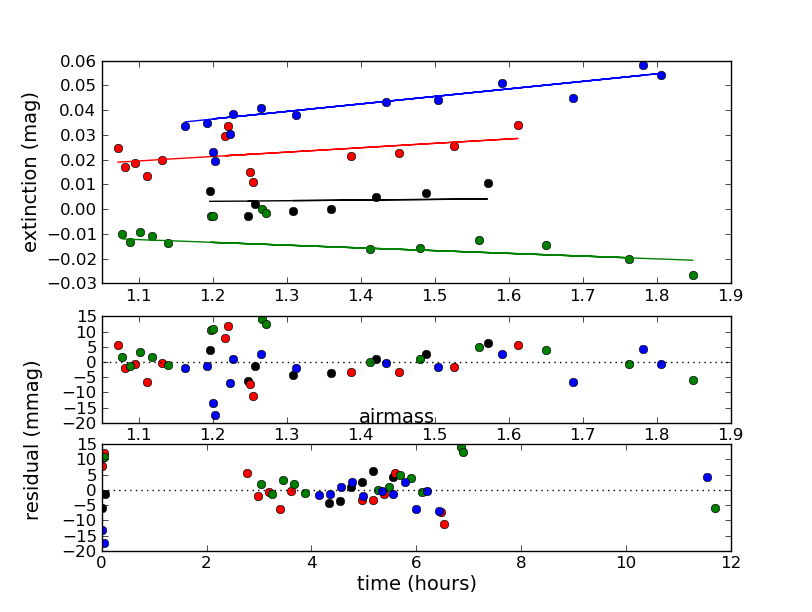
Figure 4.— The best-fit airmass terms for the November 2000 Kitt Peak run are puzzling. See text for details.

We stress that these examples are interesting precisely because they are atypical. Most runs show no such unexpected behavior, yielding fits similar to the uppermost three nights in Figure 3 and residuals similar to the lower panels of that figure. The atmospheric variations are often modeled to within a few millimagnitudes over a wide range of airmass. Figure 5 shows histograms of the exposure residuals in each filter, for exposures in photometric conditions (recall that the residual is identically zero for exposures in nonphotometric conditions). These histograms indicate that a simple airmass term is sufficient to model many hundreds of photometric exposures to within $\sim 5$ mmag.

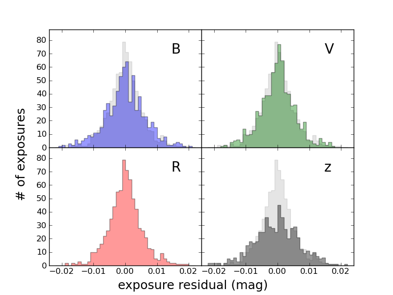
Figure 5.— Histograms of the exposure residuals in each filter, for exposures in photometric conditions. The $R$ histogram is superposed on the $BVz$ histograms for comparison.

4.2. Run Zeropoints

Figure 6 shows the run zeropoints for each run with at least one photometric night in a given filter. Only relative zeropoints are meaningful, and only within a given filter. The most striking feature is that the four filters vary so nearly in unison, especially at CTIO, despite the completely independent fit in each filter. This, along with the month-to-month stability, suggests that the variations reflect real long-term changes rather than noise. (The referencing of the zeropoint to the center of CCD 1 rather than to an average over the entire array causes only $\lesssim$0.02 mag shifts in this plot, which we neglect hereafter.)

Figure 6.— Run zeropoints, as defined in Equation 1, for each run with at least one photometric night in a given filter ($B$, blue; $V$, green; $R$, red; ${z}$, black) at Kitt Peak (left) and Cerro Tololo (right).

Because the zeropoint appears on the right side of Equation 1 rather than on the left, an increase in zeropoint implies lower pixel values for a given star (this is contrary to how observational astronomers usually think about a zeropoint). Upward excursions in zeropoint could be caused by decreases in the atmosphere-independent part of the throughput, higher CCD amplifier gain (i.e., lower pixel value per photoelectron in the device), or similar factors. The variations do not appear to be correlated with recoatings of the optics at CTIO (A. Walker, private communication). We do have evidence of undocumented gain changes on shorter timescales (§4.1), so longer-term drifts in gain could be responsible for the coherent part of the time variation. However, because the variation at shorter wavelengths is larger than at longer wavelengths, this cannot be the entire explanation. Wavelength-dependence suggests a physical cause, and the blueness of the effect rules out some physical causes such as CCD temperature changes. We conclude that there are long-term ($\sim$2-year) variations in hardware throughput due to as-yet unexplained causes.

4.3. Flatfield Corrections

Figure 7 shows the flatfield corrections in magnitudes, averaged over all runs at Kitt Peak (left column) and nearly all runs at Cerro Tololo (right column), in $B$, $V$, $R$, and ${z}$ (top row to bottom row). This is a visualisation of the last term in Equation 1, so a larger positive number means that a star in the sky-flattened images appears fainter than it would have if the sky flats had been perfect. The variation from run to run is much smaller than the systematic differences between telescopes and among filters, so we begin by discussing those patterns:

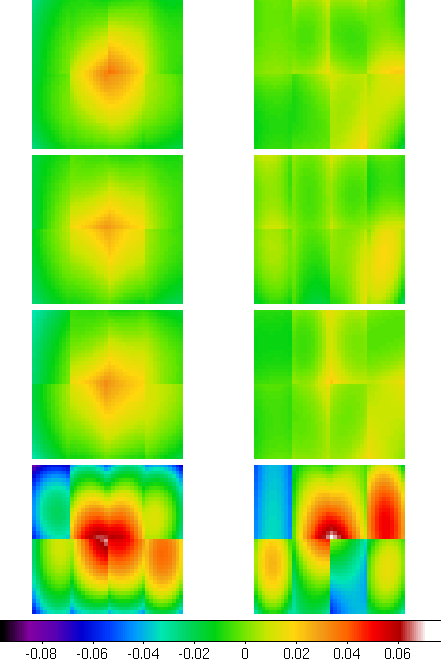
Figure 7.— Flatfield corrections in magnitudes for Mosaic at Kitt Peak (left column) and Mosaic 2 at Cerro Tololo (right column), in $B$, $V$, $R$, and ${z}$ (top row to bottom row). Each image is a mean over many observing runs; the variation from run to run is much smaller. See text for physical interpretation.

1. The Kitt Peak and Cerro Tololo corrections clearly form two different families. We stress that there is nothing in the model to enforce or even suggest that this should be the case. Each run has its own set of flatfield parameters, unconnected to the other runs. The fact that the flatfield parameters for the Cerro Tololo runs are similar to each other and dissimilar to those for the Kitt Peak runs is therefore due entirely to the data rather than the model. This gives us confidence that the solution is representing real systematic errors in the flatfielding.

2. In BVR, the corrections are more or less continuous across CCDs. Again, we stress that this is not required or encouraged by the model, and the fact that data prefer it suggests that the data are responding to physical effects which operate mostly on Mosaic-wide scales. However, ${z}$ band is not very contiguous because it is very sensitive to CCD thickness, which is obviously not continuous at the boundaries. Because there can be real discontinuities, we retain the chip-by-chip model despite the dominance of the larger-scale patterns.

3. At each observatory, $B$, $V$, $R$ are similar to each other and very different from ${z}$ band, which has by far the biggest corrections. Again, this was not suggested by the model, which is completely independent in each filter.

We attribute the differences between ${z}$ and BVR to physical factors. First, across the ${z}$ band the CCD sensitivity is a strong function of CCD thickness and wavelength. The discontinuous nature of the ${z}$ band corrections is likely due to varying device thickness. Second, the larger amplitude of the radial pattern in ${z}$ may be due to the effective wavelength of the ${z}$ filter changing across the field, because it is an interference filter.

Although the hardware setups at Kitt Peak and Cerro Tololo are quite similar, they are not identical. The telescopes have different prime focus correctors, and some differences in the raw images produced by Mosaic and Mosaic 2 are evident upon casual inspection, depending on wavelength. Thus it is not surprising to see telescope- and wavelength-dependent systematics reflecting our inability to completely remove these effects in the image processing. The fact that the data, unguided by the model, produce the physically plausible patterns listed above lends confidence to the results.

The sign of the central pattern seen in the Kitt Peak corrections can be interpreted as follows. If there are too many sky photons near the center (perhaps traversing the optical system through paths which are forbidden to object photons), then dividing the raw data by the sky flats will make objects near the center appear to be too faint, which is the sign of the pattern shown here. This is about a 5% or 0.05 mag effect from center to edge in BVR, and a bit more than twice as large in ${z}$. In ${z}$ band at Kitt Peak an additional complication is the presence in raw images of a ghost image of the pupil, covering much of the array and with an amplitude $\sim$3% of the sky. Mosaic ${z}$ images are therefore reduced with an extra step, the IRAF task rmpupil which attempts to model and remove this additive effect which is roughly centered on the array. Undersubtracting this feature will lead to the same sign error shown here, centered on the array. However, the ghost pupil hypothesis does not explain why the corrections derived here are sizable even in the bands where the ghost pupil is not evident. Furthermore, the amplitude of any ghost pupil image undersubtraction is likely to be negligible on the scale shown here, as only a $\sim$3% error would result in the case of no subtraction at all.

The central pattern seen in BVR at Kitt Peak is about the same amplitude as the Jacobian correction, which is also centrally symmetric. However, we rule out an incorrect Jacobian correction as the cause based on two lines of reasoning. First, the correction is applied the same way for the Cerro Tololo, which shows no such central pattern. Second, if ubercal were compensating for a mistake in the input photometry, then the corrected final images would contain the negative of this mistake. Analysis of such images (§4.4 and §5) demonstrates that this is not the case.

The usual application of sky flats is known to be wrong for another reason (Stubbs et al. 2007). Sky flats represent one integral over wavelengths, and object fluxes represent a different integral over wavelengths, but the proper correction would involve dividing the integrands, not the integrals. If this is the cause of flatfielding errors, the ubercal is performing a correction for the mean colors of the objects in the input photometry. However, given the Mosaic-wide scale and central symmetry of most of the corrections derived here, we favor an optics-related explanation for the bulk of these corrections.

For a given filter and observatory, the flatfield corrections are fairly stable over time. At a given camera location, the standard deviation across runs is typically 4-5 mmag, an order of magnitude smaller than the corrections shown here. This consistency might suggest constraining the flatfield corrections even more strongly by solving for a single pattern per observatory and wavelength. However, runs closer in time seem to be somewhat more consistent with each other, suggesting that some of the time variation is real. Therefore, we continue to model each run separately.

One striking example of variation with time is when CCD 3 at Cerro Tololo failed and was replaced. Figure 8 shows the ${z}$ correction over the whole field before and after replacement. CCD 3 has clearly changed, while the rest of the field has not changed substantially. Before replacement, the corrections for CCD 3 were just as stable from run to run as the other CCDs shown here. The BVR corrections for this CCD also changed at the same time, but are of smaller amplitude. Again, we stress that these patterns come from the data because the model knows nothing about the CCD replacement.

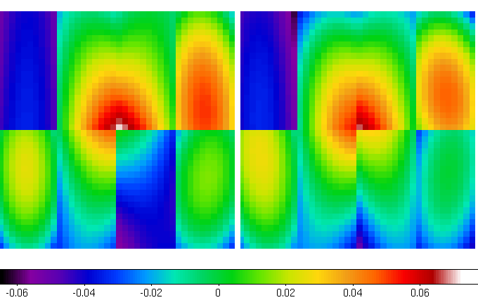
Figure 8.— Flatfield corrections for Cerro Tolo in ${z}$ before and after the replacement of CCD 3 (third from left in bottom row). As shown by the other CCDs, the flatfield corrections are generally stable over time although the model allows independent parameters for each run. This one-time change of hardware clearly shows up in the ubercal-derived corrections.

We can test the appropriateness of the polynomial model by mapping the residuals back onto camera coordinates. To build up a statistically meaningful map, we average over all runs in a given observatory/filter combination. This is shown in Figure 9 for Mosaic (left) and Mosaic 2 (right) for the filters in the usual order. At Kitt Peak, we see faint echoes of the ghost pupil, most clearly in $B$, where it is barely visible in the raw images at the $<1\%$ level but not modeled out in the image reduction stage. At Cerro Tololo, three ghost pupils are evident in most filters—a large one at the center and two smaller ones at lower right—and some additional process must be at work in $V$. Despite the clarity of these patterns, their amplitude is small, about an order of magnitude smaller than the patterns captured by the polynomial model. Their spatial frequencies are also high, so that they will be washed out by dithering. A way to capture this high spatial frequency information without adding multiple parameters would be to add a smoothed version of the appropriate map back into the flatfield model as an extra term, perhaps with a free parameter for its amplitude on each image or on each run.

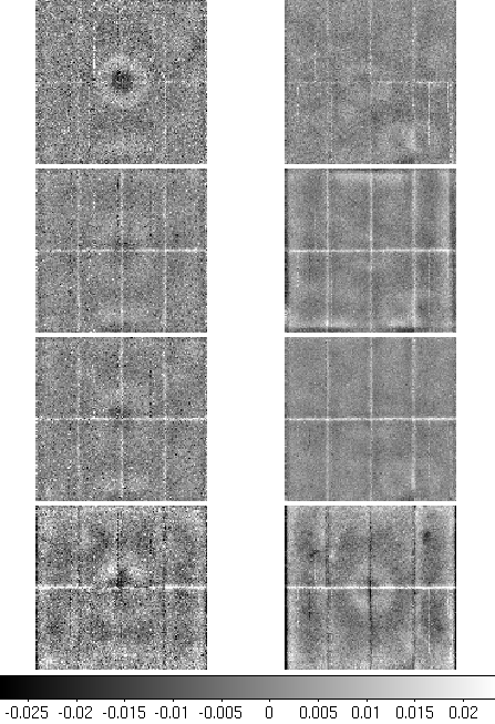
Figure 9.— Map of the residuals (in magnitudes) back onto the camera coordinates at Kitt Peak (left) and Cerro Tololo (right) for, from top to bottom, $B$, $V$, $R$, and ${z}$. For example, at Kitt Peak in $B$, objects in the center of the camera field are observed to be systematically brighter than modeled, revealing an inadequacy (at the 15 mmag level) of the second-order polynomial flatfield correction model.

A few other features in these maps are worth noting. Bad columns are visible in places, indicating that the input photometry could have been cleaned better. More interesting is the edge behavior. In BVR, objects near inside edges are consistently fainter than expected (the white bands are not depictions of the CCD gaps), but whatever causes this does not affect photometry near the outside edges. This inside/outside distinction points to a physical cause rather than a SExtractor issue. In ${z}$ the sign of the effect reverses for the long inside edges, and objects near the outside edges are now affected as well. These are small effects, but consistent across observatories, so it is presumably related to the CCDs, readout electronics, and/or image processing steps, which are largely the same at both observatories. Future surveys wishing to obtain very high precision should examine spatial patterns in the residuals and use them to refine their models.

4.4. Closing the loop

To implement the corrections, we modified our stacking software (dlscombine, Wittman et al., in preparation) to perform the flatfield corrections on the fly as it stacks. We also configured it to use the extinction corrections derived from ubercal, rather than from our previous method of estimating extinction corrections.

We tested the corrections by having dlscombine write out corrected postage-stamp images for each observation of each ubercal object. This is an end-to-end test involving many interrelated pieces, such as applying the correct Jacobian determinant to the ubercal input catalogues so that the combination of flatfield corrections and repixelisation produces uniform photometry. We photometered the postage stamps using the same procedure as for the ubercal input catalogues, and subtracted the model true magnitude for each object. The resulting residuals should have zero mean, with rms similar to the rms residuals found in the ubercal fit. More importantly, any subset of residuals should have zero mean, so we can subdivide the data by field, subfield, CCD, etc, and check for systematics. None of these attributes show any significant trends. For example, Figure 10 shows histograms of the ${z}$ band residuals for the end-to-end test in field F2, subdivided by CCD. There is no evidence for a systematic offset in any CCD. A similar comparison of fields yields no evidence for field-to-field offsets either.

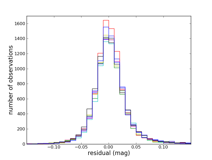
Figure 10.— Histogram of residuals in the end-to-end test for field F2 in ${z}$ band, with each CCD in the Mosaic represented by a different color. Systematic offsets between CCDs, if any, must be very small.

The residual measured for any observation of any object with the end-to-end test is very well predicted by the model residuals in ubercal itself. For example, if the ubercal fit left a +0.05 mag residual for a particular observation of a given star, we find that the measured magnitude of that star in that observation’s corrected postage-stamp image is indeed 0.05 mag fainter than the measured magnitude of the same star in its other corrected postage-stamp images. The error is thus in the modeling, not in the application of the corrections, although applying the corrections and re-photometering does add some ($\sim$ 0.01-0.02 mag) extra scatter. Thus, Figure 10 is just a slightly broadened histogram of the residuals estimated by ubercal itself. The resulting confidence in the model residuals is a key feature for rapid refinement of the modeling process. We can much more quickly search the model residuals for patterns than we can apply the corrections and search the corrected photometry for patterns.

The software used to produce the final DLS stacks is identical to that used for the end-to-end tests, with only minor changes in the output configuration to facilitate the postage-stamp analysis. Thus the procedure should (and in fact did; see §5) greatly improve the uniformity of the photometry in the DLS stacks. Nevertheless, two processes which do affect the final DLS photometry are not tested by the methods of this section. First is the actual coaddition of pixels from different exposures. The coaddition of images with different point-spread functions (PSFs) introduces issues which are explicitly not tested here. Second, the method of producing catalogues from the DLS stacks differs from the method used for photometry here, because the prime consideration in constructing the DLS catalogues is consistent measurement of colors, which involves the PSFs of all the bands, whereas ubercal deals with only one at a time. These issues are discussed in more detail in the DLS data release paper (Wittman et al., in preparation). Despite these details, ubercal was by far the most important step for making the DLS photometry uniform.

4.5. Robustness

The results presented above are robust against marginal changes in the model. For example, for those nights which are borderline nonphotometric, the flatfield corrections do not change substantially when the status of the night is changed from photometric to nonphotometric or vice versa. Another type of model change discussed above was the use of SDSS photometry to fix the magnitudes of a subset of objects. This too did not alter the basic results.

However, ubercal is only as good as its input photometry. If the input photometry is biased in some way, then the results will be precisely wrong. The most obvious kind of bias is seeing dependence. If the photometry is not very robust against seeing changes, it may capture a smaller fraction of the light in poor seeing conditions, and thus ubercal will overestimate the extinction in those exposures. After correction by ubercal, those exposures will be too bright. We searched for this effect in two ways. First, we looked for correlations between seeing and airmass terms on photometric nights, and found no evidence for such correlations. Second, we checked the final photometry on the stacked images (after all corrections, as described below) and compared the stellar locus in color-color space between subfields which on average had good seeing in ${z}$ and those which had poor seeing in ${z}$. (Due to the observing strategy, ${z}$ had the biggest seeing variations, so the other bands served as relatively stable references for this test.) We did not find any indication that ubercal was fed seeing-dependent photometry.

Because ${z}$ band has the biggest seeing variations, has the least-clean ubercal fit, and shows the biggest variations in the final stacked photometry, we probed the systematics of its ubercal input photometry two more ways. First, we analyzed the fit residuals of stars and galaxies independently. For each exposure, we tabulated the mean residual difference between stars and galaxies and performed a regression against seeing and sky noise. There was a trend with seeing, such that stars were measured to be 3 mmag brighter in the best seeing compared to typical seeing, 3 mmag fainter in 10th percentile (i.e. nearly the worst) seeing, and up to 7 mmag fainter in the very worst seeing. The trend with sky rms was of a similar size but opposite sign: increased sky noise penalizes galaxies more than stars. Thus the input photometry does contain systematic errors, but at a level lower than we are concerned with here.

Second, we made a completely new and independent ${z}$ input catalogue using a different algorithm, PSF fitting, which should be robust against losing a larger fraction of object light in poor seeing. For each CCD of each ${z}$ exposure, we compiled a list of point sources by drawing a rectangular box around the stellar locus in size-magnitude space. Note that “point source” here refers to appearance on a specific exposure. If a bright star is saturated in some exposures but not in others, it is considered a point source for these purposes only in the latter. We threw out observations with peak flux 80% or more of the already-cautious nominal saturation level. We also imposed a minimum peak flux of 500 ADU, for a peak S/N of about 10, to avoid wasting time fitting low S/N stars. We then fit elliptical Gaussians to each point source, throwing out those which failed to converge and those where the centroid shifted from the original SExtractor position by more than two pixels (which could indicate a problem such as a close neighbor).

After running ubercal on this input photometry, we found that the mean flatfield corrections were nearly identical to those for the original set of photometry. More importantly, we restacked the subfield with the most extreme seeing variations in ${z}$ ($\sim$0.9-1.5${}^{\prime\prime}\,$ FWHM) and found no substantial change in the photometry relative to SDSS. We conclude that the corrections derived here are robust against seeing variations and robust against changes in the procedure used to assemble the input photometry.

5. Impact on DLS

Prior to running ubercal, the DLS stacks in ${z}$ showed large ($\sim$20%) spatial variations in photometry, particularly in the fields imaged from Kitt Peak, F1 and F2. The primary test of photometric uniformity was the stellar locus in color-color space. This locus changed from subfield to subfield, not just in location but also in shape and width. Of course, color-color plots mix errors from different bands. We suspected that ${z}$ band had the largest variations, but could not prove it. Therefore, we focused on F2, which had the largest variations and where the overlap with SDSS allowed us to isolate the different bands.

We took stars from the SDSS database and used their colors to assign types. We then used the Pickles and updated Bruzual-Persson-Gunn-Stryker stellar spectral libraries to predict DLS magnitudes using the filter, detector, and telescope throughput curves. Finally, we mapped the spatial variations in calibration directly in each filter by comparing these predictions with magnitudes measured on the DLS stacks. This clearly indicated that ${z}$ had the largest variations, but that other bands had substantial variations as well.

This is consistent with the flatfield corrections subsequently derived from ubercal: The corrections for ${z}$ band are about twice as large peak-to-valley as in the other bands at Kitt Peak, and in any given band the Cerro Tololo corrections are smaller than the Kitt Peak corrections.

Figure 11 shows the F2 DLS-SDSS maps for DLS filters BVRz top to bottom, before (left) and after (right) applying ubercal to the DLS data. The spatial coordinates are now RA,DEC on the sky rather than $x,y$ on the camera, and each image represents the entire 2${}^{\circ}\times 2^{\circ}$ field, which is composed of a 3$\times$3 grid of roughly camera-sized subfields. North is up and east is left. There is now a lot of noise, because there are only about 12,000 SDSS stars in this field, each star is measured only once (on the stacked DLS image), and stars can be mistyped. Each star is one point on the map. It is clear in $R$ and ${z}$ at least that the pre-ubercal stacks objects near the centers of the subfields are fainter than objects near the edges, just as one would guess from ubercal’s flatfield corrections. This pattern is not evident in the post-ubercal data. Furthermore, the pre-ubercal data have gradients across the entire field, for example southeast to northwest in $R$ and ${z}$. These are also not evident in the post-ubercal data. Because of the removal of these patterns, residual subfield-to-subfield patterns are more evident in the post-ubercal stacks. The continued existence of some patterns may have more to do with the stack-photometry issues discussed at the end of §4.4 than with ubercal.

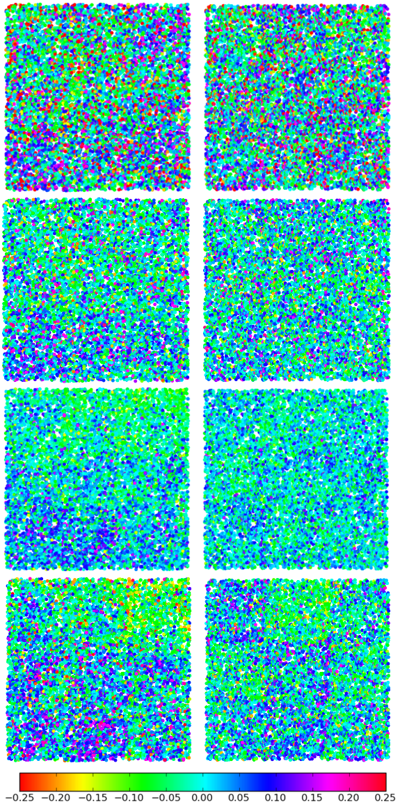
Figure 11.— DLS minus SDSS magnitudes for SDSS stars in DLS field F2. Each image represents the 2${}^{\circ}\times 2^{\circ}$ field with north up and east left. The left column of images is pre-ubercal, the right column is post-ubercal, and the rows represent, from top to bottom, BVRz. Mean values have been removed from each image so that nonuniformities can be more clearly compared. Ubercal was successful at removing the intra-subfield bowl patterns and the large-scale gradients.

The origin of the pre-ubercal large-scale gradients may be due to a camera-scale effect. Referring to ${z}$ band as a specific example, imagine the north and west sides of the camera have a photometric offset relative to the south and east sides. The north side of the camera in one subfield overlaps the south side of the camera in another subfield. When photometric offsets between subfields are determined by enforcing consistency in the overlapping objects, this camera-scale error gets replicated and amplified as subfields are stitched together across a larger field. Thus, large fields cannot be synthesised properly without accurately modeling camera-scale errors.

6. Conclusions

We have implemented a version of the global linear least squares procedure introduced by P08 (and known as ubercal) for the Deep Lens Survey. The DLS is structured very differently from SDSS, and this required a restructuring and reimplementation of the procedure. The lessons learned may be of interest for surveys structured more like the DLS, e.g., shift-and-stare rather than drift-scan.

Isolated fields. Many deep ground-based surveys have isolated fields which allow full nights to be split between a small number of fields. Our original intent was to calibrate each field against standard stars, but with ubercal we have tied the fields together first, and saved the overall calibration for last. This makes the photometry as uniform as possible. Multiple fields can be tied together directly only if they are observed on the same photometric night in the same filter. Unlike SDSS, most observers must choose one filter at a time. Therefore, when multiple fields are observed on a photometric night, observers should take care to make observations in as many relevant filters as practical.

Multiple observatories. The value of taking some observations of southern fields from the northern telescope and vice versa was not obvious at the start of the survey. But in the end it had enormous value for tying the northern and southern fields to a common system without any reference to standard stars. Thus, the observing plan for photometric nights should include a small amount of time for cross-hemisphere observing, even on fields which are not well placed for such observing. The point is not to go deep on those disadvantageous fields, but just to get some cross-calibration. Furthermore, each filter requires some cross-observing in photometric conditions. Because this was not in the original plan for the DLS, we made creative use of repeated observations of equatorial standard star fields from both observatories. For ubercal, the value is not in the standard stars themselves but merely in the fact that those fields were observed by both observatories in photometric conditions. All objects in the fields, not just the standard stars, were used for ubercal.

Shift-and-stare imaging. The SDSS flatfield corrections were one-dimensional due to the drift-scan design of SDSS. With shift-and-stare imaging, the flatfield corrections are two-dimensional and there are many more options for modeling them. Although the patterns we find are mostly smoothly varying over the focal plane, we do find some chip-to-chip discontinuities and we believe it is important to allow these in the model. For Mosaic and Mosaic 2, a second-order polynomial does reasonably well, but not perfectly. In §4.3 we offer a suggestion for capturing high spatial frequency features without introducing many new parameters.

Separately, we find that the mere existence of many dithers on a given field does not lead to good constraints on the flatfield corrections, due to a spatiotemporal degeneracy (§2.3). There must be a strong constraint on the time behavior of the throughput, which in practice means that photometric nights are key to providing these constraints.

Nonphotometric imaging: everything is connected. A substantial fraction of our imaging was taken in nonphotometric conditions. Although photometric nights are key as explained above, flatfield corrections can still be derived even for a completely nonphotometric run. This is because overlapping photometric data provide the necessary constraints. For example, if the true star magnitudes in a field are well constrained by photometric nights, then in principle one could derive flatfield corrections for any subsequent data simply by direct comparison to the true magnitudes. This should work two steps removed as well: if one field is well-constrained and a nonphotometric run includes that field as well as another field, then the flatfield corrections can be derived by comparison to the well-constrained field, and the flatfields then used to constrain the spatial pattern of true magnitudes in the second field, up to a constant offset. Of course, a global simultaneous fit is preferred to this multi-step procedure, but this illustrates conceptually how a surprising amount of information can be gleaned from interlocking observations. In summary, ubercal performed well in solving for model parameters on nonphotometric runs, as long as some relevant photometric observations were available.

Atmospheric variations. Even on photometric nights, there is a $\sim$0.01 mag variation in atmospheric throughput on $\sim$2 hour timescales. If there is a spatial component to this variation, future surveys which need to be very precise might benefit from a boresighted monitoring telescope. Data from the monitoring telescope could provide the more precise atmospheric model necessary to model out these variations.

Overall value of global fitting. Applying ubercal to the DLS revealed serious flaws in the flatfielding, and correcting these flaws resulted in much more uniform photometry, reducing the peak-to-valley variation from $\sim$0.2 mag to $\sim$0.05 mag, with most of the remainder due to the non-ubercal-related factors discussed in §4.4. Sky or dome flats are still important because they provide pixel-by-pixel characterisation, but no observer should rely on flats to accurately represent large-scale spatial sensitivity variations without an independent check such as this procedure.

Survey pipelines should always solve for these corrections to make the photometry as uniform as possible. In fact, without these corrections the synthesis of large fields from many camera pointings can be very problematic. Because the corrections are relatively consistent from run to run, they can also be included in quick-look reductions. The improvement in photometric uniformity may even be enough to influence some observing decisions such as whether a newly discovered variable object is interesting enough to warrant further followup. Surveys for which transient alerts are a data product, such as LSST, should apply recently derived corrections in their real-time reductions to improve the quality of the alerts.

Future surveys which wish to push the precision further may have to consider some more subtle effects not considered here. First, by using bright objects to derive corrections for the faint objects we are most interested in, we have assumed some some degree of linearity. Future surveys should control for this potential systematic error. Second, we have assumed that these corrections are color-independent, or at least that correcting for the typical color of ubercal objects is sufficient. Future surveys will want to control for this as well, at least by checking the color dependence if not implementing a color-dependent corection. The method of Stubbs et al. (2007) should help greatly in controlling color dependence.

The global fitting also revealed that some exposures which were apparently good upon manual inspection had some serious flaws. Global fitting thus provides a uniform, objective check on the quality of data. Recalling some of the more problematic data, it seems that large surveys contain data weirder than we suppose, but not necessarily weirder than we can suppose. Global fitting alerted us to the presence of unexpected effects such as apparent gain changes, but once these effects are recognised they can be modeled well enough to yield uniform photometry even if the ultimate physical mechanism remains unidentified.

References

- LSST Science Collaborations: Paul A. Abell et al. (2009) LSST Science Collaborations: Paul A. Abell, et al. 2009, arXiv:0912.0201
- SE (1996) Bertin, E. and Arnouts, S. 1996, A&A Supp. 117, 393
- Landolt (1992) Landolt, A. U. 1992, AJ, 104, 340
- Muller (1996) Muller, G. P., Reed, R., Armandroff, T., Boroson, T. A., & Jacoby, G. H., Proc. SPIE 3355, 577, 1998
- Padmanabhan et al. (2008) Padmanabhan, N., et al. 2008, ApJ, 674, 1217
- Pickles (1998) Pickles, A. J. 1998, PASP, 110, 863
- Press et al. (1992) Press, W. H., Teukolsky, S. A., Vetterling, W. T., & Flannery, B. P. 1992, Cambridge: University Press, —c1992, 2nd ed.,
- Smith et al. (2002) Smith, J. A., et al. 2002, AJ, 123, 2121
- Stubbs et al. (2007) Stubbs, C. W., et al. 2007, The Future of Photometric, Spectrophotometric and Polarimetric Standardization, 364, 373
- Wittman et al. (2002) Wittman, D. M., et al. 2002, Proc. SPIE, 4836, 73
- Wittman et al. (2006) Wittman, D., Dell’Antonio, I. P., Hughes, J. P., Margoniner, V. E., Tyson, J. A., Cohen, J. G., & Norman, D. 2006, ApJ, 643, 128