Time-dependent spin-wave theory

Abstract

We generalize the spin-wave expansion in powers of the inverse spin to time-dependent quantum spin models describing rotating magnets or magnets in time-dependent external fields. We show that in these cases, the spin operators should be projected onto properly defined rotating reference frames before the spin components are bosonized using the Holstein-Primakoff transformation. As a first application of our approach, we calculate the reorganization of the magnetic state due to Bose-Einstein condensation of magnons in the magnetic insulator yttrium-iron garnet; we predict a characteristic dip in the magnetization which should be measurable in experiments.

I Introduction

At low temperatures the static and dynamic properties of magnets are often determined by spin-wave excitations, which are bosonic quasiparticles in a magnetically ordered state. The theory of spin waves Akhiezer68 has been extremely successful to explain experimental data for a great variety of magnets. The basic assumption is that the thermal and quantum fluctuations are sufficiently small, so that one can expand in fluctuations around the classical ground-state configuration. The first step in the spin-wave expansion is therefore the determination of the spin configuration in the classical limit, where the spin operators are treated as classical vectors. Deviations from the classical limit can then be obtained by projecting the spin operators onto a basis which matches the direction defined by the classical spin configuration, and then bosonizing the spin components using the Holstein-Primakoff transformation. Akhiezer68 Assuming that the spin quantum number $S$ is large, one can then calculate fluctuation corrections perturbatively in powers of $1/S$.

It is not obvious how to generalize this strategy to explicitly time-dependent spin Hamiltonians, because in this case energy is not conserved and the proper basis for setting up the spin-wave expansion may not be determined by minimizing the classical ground-state energy. At the first sight one can avoid this problem by simply projecting the spin operators onto a fixed (laboratory) coordinate system and then introducing Holstein-Primakoff bosons as usual. However, as will be demonstrated below, this strategy is not suitable to describe a possible dynamic reorganization of the magnetic state. Moreover, in the laboratory basis it is often very cumbersome (and in practice impossible) to take into account the dominant fluctuation effects. In this work, we shall develop the general framework to set up a proper $1/S$ expansion out of equilibrium and then use our method to calculate the magnetization dynamics of a simplified spin model for the pumped magnon gas in the magnetic insulator yttrium-iron garnet (YIG),Cherepanov93 ; Melkov96 where parametric resonance and Bose-Einstein condensation (BEC) of magnons has recently been observed. Demokritov06

II Spin wave approach

II.1 Spin-wave expansion in equilibrium

To explain the basic principles of the time-dependent spin-wave expansion, we first consider a Heisenberg ferromagnet in a time-dependent magnetic field,

$${\cal{H}}(t) =-\frac{1}{2}\sum_{ij}J_{ij}{\bm{S}}_{i}\cdot{\bm{S}}_{j}-\sum_{i}{\bm{h}}_{i}(t)\cdot{\bm{S}}_{i},$$ (1)

where the sums are over the $N$ sites of a cubic lattice, and $\bm{S}_{i}$ are quantum mechanical spin operators localized at the lattice sites $\bm{R}_{i}$. The spins interact via exchange couplings $J_{ij}$ and are exposed to an external space- and time-dependent magnetic field $\bm{h}_{i}(t)$ which we measure in units of energy. Assuming that $\bm{h}_{i}(t)$ is sufficiently large, the nonequilibrium expectation values $\langle\bm{S}_{i}(t)\rangle$ are finite so that the time-dependent unit vectors $\bm{\hat{m}}_{i}(t)=\langle\bm{S}_{i}(t)\rangle/|\langle\bm{S}_{i}(t)\rangle|$ in the direction of the local magnetic moments are well defined. If the time-dependence of the external field is sufficiently slow, we may use the adiabatic approximation to determine $\bm{\hat{m}}_{i}(t)$. In this case we may set up the spin-wave expansion as in equilibrium Schuetz03 by projecting the spin operators onto a time-dependent basis $\{\bm{e}_{i}^{(1)}(t),\bm{e}_{i}^{(2)}(t),\hat{\bm{m}}_{i}(t)\}$, where $\bm{e}_{i}^{(1)}(t)$ and $\bm{e}_{i}^{(2)}(t)$ are time-dependent unit vectors orthogonal to $\hat{\bm{m}}_{i}(t)$. The directions $\hat{\bm{m}}_{i}(t)$ are determined by a time-dependent extension of the static minimization condition of the classical ground-state energy, Schuetz03

$$\hat{\bm{m}}_{i}(t)\times\Big{[}{\bm{h}}_{i}(t)+S\sum_{j}J_{ij}\hat{\bm{m}}_{j}(t)\Big{]}=0.$$ (2)

We then expand the spin operators as ${\bm{S}}_{i}=S^{\parallel}_{i}\hat{\bm{m}}_{i}+\frac{1}{2}[{S}_{i}^{+}{\bm{e}}^{-}_{i}+{S}_{i}^{-}{\bm{e}}^{+}_{i}]$, where ${\bm{e}}^{\pm}_{i}={\bm{e}}^{(1)}_{i}\pm i{\bm{e}}^{(2)}_{i}$. Finally, we express the spin components in terms of canonical boson operators $a_{i}$ using the Holstein-Primakoff transformation, Akhiezer68 $S_{i}^{\parallel}=S-a^{\dagger}_{i}a_{i}$, ${S}_{i}^{+}=(S_{i}^{-})^{\dagger}=[2S-a^{\dagger}_{i}a_{i}]^{1/2}a_{i}$. For large $S$ the square roots can be expanded and the interactions between spin-waves can be taken into account by means of a systematic expansion in powers $1/S$.

II.2 Spin waves in the adiabatic basis

It turns out, however, that this approach is only useful in the adiabatic limit where the rate of change of the external field is small compared with $|\bm{h}_{i}(t)|$. To see this, consider the special case of a homogeneous field $\bm{h}_{i}(t)=\bm{h}(t)$ which rotates clockwise with frequency $\omega$ around the $z$ axis,

$$\bm{h}(t)=h_{\bot}[\cos(\omega t)\hat{\bm{x}}-\sin(\omega t)\hat{\bm{y}}]+h_{z}\hat{\bm{z}}\;,$$ (3)

where $\hat{\bm{x}}$, $\hat{\bm{y}}$ and $\hat{\bm{z}}$ are unit vectors in the directions of three orthogonal axes of the laboratory. By writing footnoterot $\bm{h}(t)\cdot\bm{S}_{i}=\bm{h}(0)\cdot e^{\omega t\hat{\bm{z}}\times}\bm{S}_{i}$, we see that Eq. (1) can alternatively be interpreted as the Hamiltonian of a magnet which rotates counter-clockwise with angular velocity $\omega$ around an axis $\hat{\bm{z}}$ which is not parallel to the field, as shown in Fig. 1.

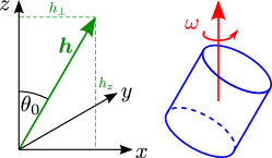
Figure 1: (Color online) Rotating magnet in a constant magnetic field $\bm{h}$ forming an angle $\theta_{0}$ with the rotation axis $\hat{\bm{z}}$ that is described by the time dependent Hamiltonian (1). The system is represented by a cylinder which is actively rotated with the constant angular velocity $\omega$ around an axis which is not parallel to the external magnetic field. The cylindrical shape and the orientation of the sample reflects the symmetry of the system at time $t=0$ where the system is rotationally invariant around the direction of the fixed magnetic field.

In adiabatic approximation the magnetization points into the direction of the magnetic field, as can be easily seen from Eq. (2). Within linear spin-wave theory we obtain the Hamiltonian

$${\cal{H}}\approx\sum_{\bm{k}}E_{\bm{k}}^{\rm ad}a_{\bm{k}}^{\dagger}a_{\bm{k}}\;,$$ (4)

where the ground-state energy has been dropped. Note that the dispersion $E_{\bm{k}}^{\rm ad}=\epsilon_{\bm{k}}+h$ is the sum of the zero-field magnon dispersion $\epsilon_{\bm{k}}=S(J_{0}-J_{\bm{k}})$ (where $J_{\bm{k}}$ is the Fourier transform of the exchange couplings $J_{ij}$) and the absolute value $h=(h_{\bot}^{2}+h_{z}^{2})^{1/2}$ of the magnetic field. Assuming that at time $t=0$ the system is in thermal equilibrium at inverse temperature $\beta=1/T$, we find that in adiabatic approximation the time-dependent magnetization $\bm{M}(t)=\frac{1}{N}\sum_{i}\langle\bm{S}_{i}(t)\rangle$ is to linear order in spin-wave theory given by

$$\bm{M}_{\rm ad}(t)=M_{h}\hat{\bm{m}}(t)\;,$$ (5)

with the magnitude of the magnetization

$$M_{h}=S-\frac{1}{N}\sum_{\bm{k}}\frac{1}{e^{\beta E_{\bm{k}}^{\rm ad}}-1}\;,$$ (6)

and its direction $\hat{\bm{m}}(t)=\sin\theta_{0}[\cos(\omega t)\hat{\bm{x}}-\sin(\omega t)\hat{\bm{y}}]+\cos\theta_{0}\hat{\bm{z}}$. Here $\theta_{0}$ is the angle between the magnetic field and the rotation axis, i.e.

$$\cos\theta_{0}=\frac{h_{z}}{h}$$ (7)

as shown in Fig. 1.

II.3 Perturbation theory in the laboratory basis

To see that Eq. (5) is only valid for $|\omega|\ll h$, let us repeat the calculation of the magnetization in a perturbative approach. To set up the spin-wave expansion we write our Hamiltonian

$${\cal{H}}(t)={\cal{H}}_{z}+{\cal{V}}(t)$$ (8)

as a sum of the time independent part

$${\cal{H}}_{z} =-\frac{1}{2}\sum_{ij}J_{ij}{\bm{S}}_{i}\cdot{\bm{S}}_{j}-h_{z}\sum_{i}S^{z}_{i},$$ (9)

and the time dependent perturbation

$${\cal{V}}(t) =-h_{\bot}\sum_{i}\left[\cos(\omega t)S^{x}_{i}-\sin(\omega t)S^{y}_{i}\right].$$ (10)

We now project the spin operators onto the fixed laboratory basis. This strategy is usually adopted to discuss parametric resonance of magnons Suhl57 ; Schloemann63 ; Zakharov70 and has recently been used in Ref. [Nakata11, ] to calculate the nonequilibrium dynamics of magnons in a related spin model. After expressing the Hamiltonian (8) in terms of laboratory-frame Holstein-Primakoff bosons $b_{i}$ and transforming to momentum space, $b_{i}=N^{-1/2}\sum_{\bm{k}}e^{i{\bm{k}}\cdot{\bm{R}}_{i}}b_{\bm{k}}$, the Hamiltonian reads in linear spin-wave theory

$${{\cal H}_{z}}\approx\sum_{\bm{k}}E_{\bm{k}}^{\rm lab}b_{\bm{k}}^{\dagger}b_{\bm{k}}^{\phantom{\dagger}}\;.$$ (11)

The dispersion $E_{\bm{k}}^{\rm lab}=\epsilon_{\bm{k}}+h_{z}$ now contains the static part of the magnetic field. The time-dependent perturbation Eq. (10) can be written as

$${\cal{V}}(t) =-\frac{h_{\bot}}{2}\sqrt{2S}\sqrt{N}\left[e^{i\omega t}b_{\bm{k}=0}^{\phantom{\dagger}}+e^{-i\omega t}b^{\dagger}_{\bm{k}=0}\right].$$ (12)

Since the boson Hamiltonian contains linear terms, the laboratory boson operators $b_{\bm{k}=0}^{\dagger}$ and $b_{\bm{k}=0}$ have finite expectation values, thus condense. The dynamics of these expectation values, as well as the time dependence of the magnon distribution function $\langle b^{\dagger}_{\bm{k}}(t)b_{\bm{k}}(t)\rangle$ can be easily obtained within linear spin-wave theory by solving the Heisenberg equations of motion. With appropriate initial conditions we obtain for the time evolution of the magnetization,

$$\bm{M}_{\rm lab}(t) =\frac{h_{\bot}S}{h_{z}-\omega}\left[\cos(\omega t)\hat{\bm{x}}-\sin(\omega t)\hat{\bm{y}}\right]+M_{h_{z}}\hat{\bm{z}}.$$ (13)

Formally the perturbation has been carried out as an expansion in powers of $h_{\perp}/h_{z}$, but we will see later that it is essentially an expansion in powers of $h_{\perp}/(h_{z}-\omega)$. An important difference to the adiabatic result (5) is the singularity for $\omega\rightarrow h_{z}$, which is of course unphysical and one would need a resummation to all orders in $1/S$ to resolve this. Using a similar approach, such a singularity has also been found in Ref. [Nakata11, ] for a slightly different model. Although for $|\omega-h_{z}|\lesssim h_{\bot}$ perturbation theory in the laboratory frame breaks down, Eq. (13) indicates that both the adiabatic approximation and the perturbative approach in the laboratory frame have serious limitations: while the adiabatic basis is restricted to slowly varying external field and misses possible dynamic instabilities, in the laboratory basis one generates unphysical singularities in linear spin-wave theory, indicating that important fluctuation effects have been neglected.

III Spin waves in the proper rotating reference frame

We now develop a time-dependent generalization of the spin-wave expansion which neither suffers from the limitations of the adiabatic approximation nor exhibits the pathologies of the perturbative approach in the laboratory frame. Our theory is guided by the following two insights: (i) the spin operators should be bosonized in a proper rotating basis whose third axis $\hat{\bm{m}}_{i}(t)$ matches the direction of the true nonequilibrium expectation value $\langle\bm{S}_{i}(t)\rangle$ and (ii) the proper rotating basis in general does not agree with the adiabatic basis defined in Eq. (2).

To construct the proper rotating basis, consider the unitary time-evolution operator ${\cal{U}}(t)$ of some arbitrary time-dependent spin Hamiltonian ${\cal{H}}(t)$, which satisfies the operator equation

$$i\partial_{t}{\cal{U}}(t)={\cal{H}}(t){\cal{U}}(t)\;.$$ (14)

Making the factorization ansatz

$${\cal{U}}(t)={\cal{U}}_{0}(t)\tilde{\cal{U}}(t)$$ (15)

with some suitable ${\cal{U}}_{0}(t)$, we find that $\tilde{\cal{U}}(t)$ satisfies $i\partial_{t}\tilde{\cal{U}}(t)=\tilde{\cal{H}}(t)\tilde{\cal{U}}(t),$ with the effective Hamiltonian

$$\tilde{\cal{H}}(t)=\tilde{\cal{H}}_{A}(t)+\tilde{\cal{H}}_{B}(t)\;,$$ (16)

where

$$\tilde{\cal{H}}_{A}(t)={\cal{U}}^{\dagger}_{0}(t){\cal{H}}(t){\cal{U}}_{0}(t)$$ (17)

corresponds to the adiabatic approximation, while

$$\tilde{{\cal{H}}}_{B}(t)=-i{\cal{U}}^{\dagger}_{0}(t)\partial_{t}{\cal{U}}_{0}(t)$$ (18)

contains all corrections to the adiabatic approximation, including possible Berry phases. Berry84 ; Bohm03 We now choose ${\cal{U}}_{0}(t)$ such that for each lattice site it rotates the $z$ axis of the laboratory to an axis in the direction $\hat{\bm{m}}_{i}(t)$ of the true local magnetization. This is achieved by setting

$${\cal{U}}_{0}(t)=e^{-i\sum_{i}\bm{\alpha}_{i}(t)\cdot{\bm{S}}_{i}}\;,$$ (19)

with suitable rotation vectors $\bm{\alpha}_{i}(t)=\alpha_{i}(t)\hat{\bm{\alpha}}_{i}(t)$, where $\alpha_{i}(t)$ is the rotation angle and $\hat{\bm{\alpha}}_{i}(t)$ is a unit vector in the direction of the rotation axis. The rotated spin operators can then be written as footnoterot

$$\tilde{\bm{S}}_{i}(t)=e^{i\bm{\alpha}_{i}(t)\cdot{\bm{S}}_{i}}\bm{S}_{i}e^{-i\bm{\alpha}_{i}(t)\cdot{\bm{S}}_{i}}=e^{\bm{\alpha}_{i}(t)\times}\bm{S}_{i}\;.$$ (20)

To calculate the corresponding Berry-phase contribution $\tilde{\cal{H}}_{B}(t)$ to the effective Hamiltonian in the rotating reference frame, we use Feynman’s Feynman51 representation

$$\frac{d}{dt}e^{A}=\int_{0}^{1}d\lambda e^{\lambda A}\frac{dA}{dt}e^{(1-\lambda)A}$$ (21)

of the time derivative of the exponential of an operator $A$ which does not necessarily commute with its time derivative $dA/dt$. It is convenient to decompose a general rotation into three successive rotations parametrized by the usual Euler angles $\varphi$, $\theta$ and $\psi$ as follows,

$$e^{\bm{\alpha}_{i}(t)\times}=e^{{\bm{\psi}}_{i}(t)\times}e^{{\bm{\theta}}_{i}(t)\times}e^{{\bm{\varphi}}_{i}(t)\times}\;,$$ (22)

where the rotation vectors are $\bm{\varphi}_{i}(t)=\varphi_{i}(t)\hat{\bm{z}}$, $\bm{\theta}_{i}(t)=\theta_{i}(t)\hat{\bm{\theta}}_{i}(t)$, and $\bm{\psi}_{i}(t)=\psi_{i}(t)\hat{\bm{m}}_{i}(t)$. McCauley97 Explicitly, the direction of the nutation vector $\bm{\theta}_{i}$ is $\hat{\bm{\theta}}_{i}(t)=\frac{\hat{\bm{z}}\times\hat{\bm{m}}_{i}(t)}{|\hat{\bm{z}}\times\hat{\bm{m}}_{i}(t)|}$. To define the spin waves in the proper rotating basis, we expand the rotated spin operators $\tilde{\bm{S}}_{i}$ defined in Eq. (20) in the time-dependent right-handed basis formed by the following three unit vectors:

$$\tilde{\bm{e}}^{(1)}_{i}(t) = \cos\psi_{i}(t)\hat{\bm{\theta}}_{i}(t)+\sin\psi_{i}(t)\hat{\bm{m}}_{i}(t)\times\hat{\bm{\theta}}_{i}(t),\hskip 19.91692pt$$ (23a)

$$\tilde{\bm{e}}^{(2)}_{i}(t) = -\sin\psi_{i}(t)\hat{\bm{\theta}}_{i}(t)+\cos\psi_{i}(t)\hat{\bm{m}}_{i}(t)\times\hat{\bm{\theta}}_{i}(t),\hskip 19.91692pt$$ (23b)

and $\hat{\bm{m}}_{i}(t)$. The corresponding spin components are defined by

$$\tilde{\bm{S}}_{i}(t)=\tilde{S}^{(1)}_{i}\tilde{\bm{e}}^{(1)}_{i}(t)+\tilde{S}^{(2)}_{i}\tilde{\bm{e}}^{(2)}_{i}(t)+\tilde{S}^{\parallel}_{i}\hat{\bm{m}}_{i}(t).$$ (24)

Evaluating the time derivative in Eq. (18) with the help of the formula (21) and inserting the expansion (24) for the rotated spin operators we can rewrite the Berry-phase contribution to the effective Hamiltonian as

$$\tilde{{\cal{H}}}_{B}(t)=-\sum_{i}\Bigl{[}\omega_{i}^{(1)}(t)\tilde{S}^{(1)}_{i}+\omega_{i}^{(2)}(t)\tilde{S}^{(2)}_{i}+\omega_{i}^{\parallel}(t)\tilde{S}^{\parallel}_{i}\Bigr{]},$$ (25)

where the three time-dependent energies $\omega_{i}^{(1)}(t)$, $\omega_{i}^{(2)}(t)$, and $\omega_{i}^{\parallel}(t)$ can be identified with the well known Euler angle parametrization of the components of the angular velocity vector in the rotating reference frame:McCauley97

$$\omega_{i}^{(1)}(t) = \dot{\varphi}_{i}\sin\theta_{i}\sin\psi_{i}+\dot{\theta}_{i}\cos\psi_{i},$$ (26a)

$$\omega_{i}^{(2)}(t) = \dot{\varphi}_{i}\sin\theta_{i}\cos\psi_{i}-\dot{\theta}_{i}\sin\psi_{i},$$ (26b)

$$\omega_{i}^{\parallel}(t) = \dot{\varphi}_{i}\cos\theta_{i}+\dot{\psi_{i}}.$$ (26c)

In the models discussed in this work the proper rotation of the comoving basis is irrelevant, so that we may focus on the special case $\bm{\psi}_{i}(t)=0$. The Berry-phase Hamiltonian (25) then reduces to

$$\tilde{{\cal{H}}}_{B}(t)=-\sum_{i}\Bigl{[} \dot{\theta}_{i}\tilde{S}^{(1)}_{i}+\dot{\varphi}_{i}\sin\theta_{i}\tilde{S}^{(2)}_{i}+\dot{\varphi}_{i}\cos\theta_{i}\tilde{S}^{\parallel}_{i}\Bigr{]}.$$ (27)

For the rotating ferromagnet shown in Fig. 1, symmetry suggests that the proper rotating coordinate system is characterized by a time-dependent precession angle $\varphi_{i}(t)=-\omega t$ and a constant nutation angle $\theta$. The Berry-phase contribution (27) to the Hamiltonian in the rotating basis is then

$$\tilde{{\cal{H}}}_{B}=\omega\sum_{i}[\sin\theta\tilde{S}^{(2)}_{i}+\cos\theta\tilde{S}^{\parallel}_{i}]\;,$$ (28)

which is independent of time. Next we express the spin components in the rotating reference frame in terms of a third type of Holstein-Primakoff boson $c_{i}$, which should not be confused with the Holstein-Primakoff boson $a_{i}$ introduced in the adiabatic basis, and also not with the laboratory basis Holstein-Primakoff boson $b_{i}$. The true tilt angle $\theta$ is determined from the requirement that the effective Hamiltonian contains no terms linear in the bosons, which yields the frequency-dependent result

$$\cos\theta=\frac{h_{z}-\omega}{\tilde{h}_{\omega}}$$ (29)

where

$$\tilde{h}_{\omega}=[h_{\bot}^{2}+(h_{z}-\omega)^{2}]^{1/2}.$$ (30)

Note that for finite $\omega$ the true tilt angle $\theta$ is larger than the angle $\theta_{0}$ between rotation axis and magnetic field. In fact, our result for $\theta$ agrees with the result for a single isolated spin in a rotating magnetic field given in the book by Bohm et al. Bohm03 For the specific geometry shown in Fig. 1 the proper rotating reference frame has also been discussed previously in Ref. [Lin05, ], but our Eq. (27) is more general. In fact, our many-body approach allows us to set up a systematic $1/S$ expansion and calculate the thermodynamics and the correlation functions of any time-dependent spin model with finite local moments. Following the steps of the spin-wave expansion we obtain the Hamiltonian

$${{\cal H}}\approx\sum_{\bm{k}}E_{\bm{k}}c_{\bm{k}}^{\dagger}c_{\bm{k}}$$ (31)

to quadratic order in the bosonic operators $c_{\bm{k}}^{\dagger}$ and $c_{\bm{k}}$ describing bosons in the proper rotating reference frame. The dispersion $E_{\bm{k}}=\epsilon_{\bm{k}}+\tilde{h}_{\omega}$ is modified by the finite oscillation frequency, see inset in Fig. 2. Imposing suitable initial conditions for our model, we obtain for the time-dependent magnetization in linear spin-wave theory,

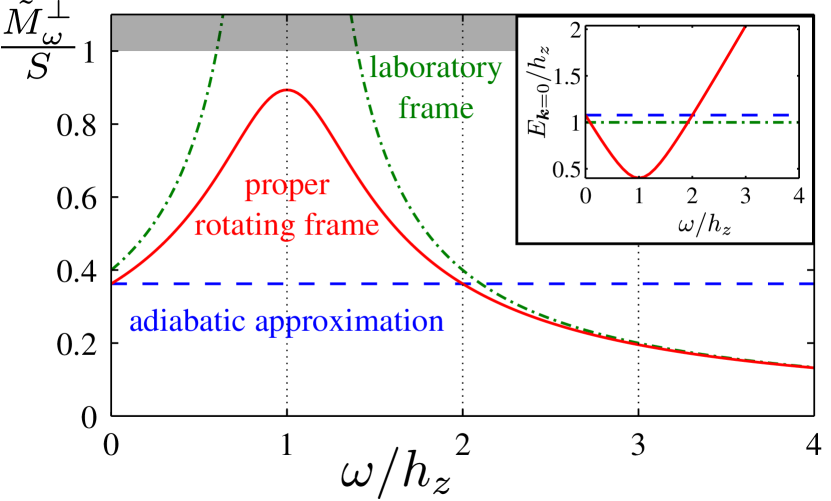
Figure 2: (Color online) Comparison of the results for the perpendicular magnetization $\tilde{M}_{\omega}^{\perp}$ as a function of the rotation frequency $\omega$ in the three different approaches for our model system given in Eq. (1) with the parameters $J=h_{z}$, $h_{\perp}=0.4h_{z}$, $S=1/2$ at the temperature $T=0.5h_{z}$: blue (dashed) line presents the results of the adiabatic approximation, Eq. (5), green (dash-dotted) line is perturbation theory in the laboratory frame, Eq. (13) and red (solid) is the proper rotating frame. The shaded area indicates the unphysical region. The inset shows a sketch of the spin-wave gap $E_{\bm{k}=0}/h_{z}$ as a function of rotation frequency for the same parameters.

$$\bm{M}(t) =\tilde{M}_{\omega}^{\parallel}\hat{\bm{z}}+\tilde{M}_{\omega}^{\perp}[\cos(\omega t)\hat{\bm{x}}-\sin(\omega t)\hat{\bm{y}}]$$

$$=\hat{\bm{m}}_{\omega}(t)\tilde{M}_{\omega}\;,$$ (32)

where $\tilde{M}_{\omega}^{\parallel}=\cos\theta\tilde{M}_{\omega}$ and $\tilde{M}_{\omega}^{\perp}=\sin\theta\tilde{M}_{\omega}$ with

$$\tilde{M}_{\omega}=S-\frac{1}{N}\sum_{\bm{k}}\frac{1}{e^{\beta E_{\bm{k}}}-1}\;,$$ (33)

and $\hat{\bm{m}}_{\omega}(t)=\sin\theta[\cos(\omega t)\hat{\bm{x}}-\sin(\omega t)\hat{\bm{y}}]+\cos\theta\hat{\bm{z}}$. In the limit $\omega\rightarrow 0$, Eq. (32) reduces to the result (5) of the adiabatic approximation, which is only accurate as long as $|\omega|\ll h$. In fact, for the two special cases $\omega=0$ and $\omega=2h_{z}$ where the effective field is equal to the external field $h=\tilde{h}_{\omega}$, the adiabatic approximation Eq. (32) matches the correct result of Eq. (5). While the result (13) for the magnetization obtained from perturbation theory in the laboratory basis approaches the more accurate rotating reference frame result (32) for $\omega\rightarrow 0$ and for large frequencies $\omega\gtrsim 2h_{z}$, perturbation theory in the laboratory basis gives unphysical results in the vicinity of the resonance $|h_{z}-\omega|\lesssim h_{\bot}$ and is thus meaningless, whereas Eq. (32) predicts that the magnetization simply rotates in the $xy$-plane ($\theta\approx\pi/2$). Note that the magnetization shown in Fig. 2 does not approach $\tilde{M}_{\omega}^{\perp}=S$ because thermal fluctuations suppress the total magnetic moment.

IV Parametric resonance and BEC of magnons in YIG

Next, let us study another time-dependent spin model which gives us some insight into the relation between parametric resonance, BEC of magnons, and the reorganization of the magnetic state. Previously, this problem has been addressed in Refs. [Zvyagin85, ; Zvyagin07, ] using a Heisenberg ferromagnet with static single-ion anisotropy in a time-dependent magnetic field. For our purpose it is more convenient to consider a modified version of this model, involving a static magnetic field in $z$ direction and a rotating single-ion anisotropy of magnitude $A$,

$${\cal{H}}(t) =-\frac{1}{2}\sum_{ij}J_{ij}\bm{S}_{i}\cdot\bm{S}_{j}-h\sum_{i}S_{i}^{z}$$

$$-\frac{A}{2}\sum_{i}\left\{[\bm{S}_{i}\cdot\bm{n}(t)]^{2}-[\bm{S}_{i}\cdot(\hat{\bm{z}}\times\bm{n}(t))]^{2}\right\},$$ (34)

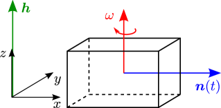
Figure 3: (Color online) Graph of the time dependent spin model defined in Eq. (34). The model can be interpreted as a Heisenberg magnet with a single-ion anisotropy axis $\hat{\bm{n}}$ that is fixed in the laboratory frame. The magnet is exposed to a static external field perpendicular to the anisotropy axis and rotates counter-clockwise around an axis parallel to the field.

where the anisotropy axis $\bm{n}(t)=\cos(\omega t)\hat{\bm{x}}-\sin(\omega t)\hat{\bm{y}}$ rotates clockwise in the $xy$ plane. An illustration of the model (34) is shown in Fig. 3. After bosonization of the spins using the Holstein-Primakoff transformation in the laboratory basis, we obtain in linear spin-wave theory,

$${\cal{H}}(t)\approx\sum_{\bm{k}}\Bigl{[}(\epsilon_{\bm{k}}+h)b^{\dagger}_{\bm{k}}b_{\bm{k}}+\frac{h_{c}}{2}(e^{2i\omega t}b_{-\bm{k}}b_{\bm{k}}+\mbox{H.c.})\Bigr{]},$$ (35)

with $h_{c}=AS$. Time-dependent boson models of this form have been studied as model systems for parametric resonance in magnon gases. Akhiezer68 ; Schloemann63 ; Zakharov70 In fact, with appropriate replacements footnoteYIG the magnon Hamiltonian for YIG in an external microwave field parallel to the external field has the same form as Eq. (35). It is well known Zakharov70 that the Hamiltonian (35) predicts a parametric instability of the magnons with wave-vectors in the regime $h_{c}>|\epsilon_{\bm{k}}+h-\omega|$. If this condition is satisfied, then the magnon occupation grows exponentially during some intermediate time interval, until it saturates and the system approaches a new equilibrium state, which in principle can be calculated by taking the interactions between the magnons into account. Here we show that the dynamics of the local magnetization $\langle{\bm{S}}_{i}(t)\rangle$ as well as the magnon spectrum can be obtained using our time-dependent spin-wave formalism without considering interactions between magnons. Because the Hamiltonian (35) has the same spin symmetries as the rotating ferromagnet discussed above, the proper rotating reference frame is again given by a time-dependent precession angle $\varphi_{i}(t)=-\omega t$ and a constant nutation angle $\theta$. The Berry-phase Hamiltonian $\tilde{{\cal{H}}}_{B}=\omega\sum_{i}[\sin\theta\tilde{S}^{(2)}_{i}+\cos\theta\tilde{S}^{\parallel}_{i}]$ is therefore identical with the rotating ferromagnet discussed above, see Eq. (28). It is then easy to show that for $|h-\omega|>h_{c}$ all spins point in the direction of the field so that the tilt angle $\theta$ vanishes and the magnon spectrum is

Figure 4: Plot of the spin-wave gap $E_{\bm{k}=0}$ of the time-dependent spin model defined in Eq. (34) as a function of $|h-\omega|/h_{c}$.

$$E_{\bm{k}}=\sqrt{(\epsilon_{\bm{k}}+h-\omega)^{2}-h_{c}^{2}}\;,$$ (36)

where again $\epsilon_{\bm{k}}=S(J_{0}-J_{\bm{k}})$. On the other hand, for $|h-\omega|<h_{c}$ the angle between magnetic field and magnetization does not vanish,

$$\cos\theta=\frac{h-\omega}{h_{c}}\;,$$ (37)

and the magnon spectrum is

$$E_{\bm{k}}^{2}=\sqrt{\Bigl{[}\epsilon_{\bm{k}}+\frac{3h_{c}}{2}-\frac{(h-\omega)^{2}}{2h_{c}}\Bigr{]}^{2}-\Bigl{[}\frac{h_{c}}{2}+\frac{(h-\omega)^{2}}{2h_{c}}\Bigr{]}^{2}}.$$ (38)

A graph of the spin-wave gap $E_{\bm{k}=0}$ is presented in Fig. 4. In the tilted phase, the time-dependent magnetization is in linear spin-wave theory $\bm{M}(t)=\tilde{M}_{\omega}\hat{\bm{m}}_{\omega}(t)$, where $\hat{\bm{m}}_{\omega}(t)=\sin\theta[\cos(\omega t)\hat{\bm{x}}-\sin(\omega t)\hat{\bm{y}}]+\cos\theta\hat{\bm{z}}$ and

$$\tilde{M}_{\omega} =S+\frac{1}{2}-\frac{1}{N}\sum_{\bm{k}}\frac{1}{E_{\bm{k}}}\Bigl{[}\epsilon_{\bm{k}}+\frac{3h_{c}}{2}-\frac{(h-\omega)^{2}}{2h_{c}}\Bigr{]}$$

$$\hskip 79.6678pt\times\Bigl{[}\frac{1}{e^{\beta E_{\bm{k}}}-1}+\frac{1}{2}\Bigr{]}.$$ (39)

Note that the gap $E_{\bm{k}=0}$ of the magnon energy vanishes at the critical fields $h_{c}^{\pm}=\pm h_{c}+\omega$, signaling a quantum phase transition. Because the magnetic state in the tilted phase spontaneously breaks the $Z_{2}$-symmetry $\bm{S}_{i}\cdot\bm{n}\rightarrow-\bm{S}_{i}\cdot\bm{n}$ of the spin Hamiltonian (34), this phase transition belongs to the Ising universality class. If we bosonize the spin operators in the laboratory frame, then at the critical point the corresponding bosons acquire a macroscopic expectation value, which corresponds to BEC of magnons. Matsubara56 ; Batyev84 However, as pointed out by Kohn and Sherrington, Kohn70 such a transition is neither accompanied by magnon superfluidity nor by off-diagonal long-range order, which distinguishes the magnon condensate from the BEC of trapped atoms or molecules. In fact, the macroscopic occupation of magnon modes is an artifact of working in the laboratory frame; the magnons defined in the proper rotating reference frame never condense.

Given the fact that our model Hamiltonian (34) has the same symmetries as the effective spin Hamiltonian for YIG, Cherepanov93 with appropriate substitutions footnoteYIG our model can be used to understand the nonequilibrium dynamics of the magnetization in YIG in the vicinity of the condensation transition. In Fig. 5, we show a numerical evaluation of the frequency-dependent magnetization $\tilde{M}_{\omega}$ given in Eq. (39) using effective parameters for YIG. footnoteYIG

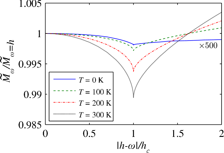
Figure 5: (Color online) Length $\tilde{M}_{\omega}$ of the magnetization vector defined in Eq. (38) at different temperatures $T$ for typical parameters describing the pumped magnon gas in bulk YIG footnoteYIG ($J=1.29~{}\mathrm{K}$, $h_{c}=0.55~{}\mathrm{K}$, $S=14.2$). The Curie temperature of YIG is $T_{c}=560~{}\mathrm{K}$. Cherepanov93 ; Melkov96 Note that for $T<T_{c}$ the magnetization in three dimensions is finite for all values of the reduced magnetic field $h-\omega$. The deviation of the $T=0~{}\mathrm{K}$ result from unity is enhanced by a factor of 500.

We predict that close to the threshold of BEC the magnetization shows a characteristic dip of the order of $1\%$ at relevant temperatures.

V Conclusions

In summary, we have developed a general method to set up the spin-wave expansion for time-dependent spin models. Our method is very general and should also be useful to study nonequilibrium phenomena in all kinds of ordered magnets, including quantum antiferromagnets and frustrated magnets with finite local moments. We have used our method to study a simplified spin model for the magnon gas in YIG, and have shown that magnon BEC in this system can be interpreted as a magnetic quantum phase transition belonging to the Ising universality class. Our prediction of a dip in the magnetization close to the threshold for BEC can be tested experimentally.

We thank M. Taillefumier, V. Vasyuchka, and A. Serga for discussions. This work was financially supported by the DFG via SFB/TRR 49.

References

- (1) A. I. Akhiezer, V. G. Bar’yakhtar, and S. V. Peletminskii, Spin Waves (North Holland, Amsterdam, 1968).
- (2) V. Cherepanov, I. Kolokolov, and V. L’vov, Phys. Rept. 229, 81 (1993).
- (3) A. G. Gurevich and G. A. Melkov, Magnetization Oscillations and Waves (CRC Press, Boca Raton, 1968).
- (4) S. O. Demokritov et al., Nature (London) 443, 430 (2006).
- (5) F. Schütz, M. Kollar, and P. Kopietz, Phys. Rev. Lett. 91, 017205 (2003).
- (6) We use the so-called Rodrigues formula to represent the rotation of a vector around an axis with angle in terms of an exponentiated cross product.
- (7) H. Suhl, J. Phys. Chem. Solids 1, 209 (1957).
- (8) E. Schlömann and J. J. Green, J. Appl. Phys. 34, 1291 (1963).
- (9) V. E. Zakharov, V. S. L’vov, and S. S. Starobinets, Zh. Eksp. Teor. Fiz. 59, 1200 (1970) [Sov. Phys. JETP 32, 656 (1971)].
- (10) K. Nakata and G. Tatara, J. Phys. Soc. Jpn. 80, 054602 (2011).
- (11) M. V. Berry, Proc. Roy. Soc. London A392, 45 (1984); B. Simon, Phys. Rev. Lett. 51, 2167 (1983).
- (12) A. Bohm et al., The Geometric Phase in Quantum Systems, (Springer, Berlin, 2003).
- (13) Q.-G. Lin, Commun. Theor. Phys. (Beijing) 43, 621 (2005).
- (14) R. P. Feynman, Phys. Rev. 84, 108 (1951).
- (15) See, for example, J. L. McCauley, Classical Mechanics (Cambridge University Press, Cambridge, 1997).
- (16) A. A. Zvyagin and V. M. Tsukernik, Fiz. Nizk. Temp. 11, 88 (1985) [Sov. J. Low Temp. Phys. 11, 47 (1985)].
- (17) A. A. Zvyagin, Fiz. Nizk. Temp. 33, 1248 (2007) [Sov. J. Low Temp. Phys. 33, 948 (2007)].
- (18) The magnon Hamiltonian for YIG in an oscillating magnetic field parallel to the static external field can be obtained from Eq. (35) by replacing by the magnon dispersion of YIG and setting . Here can be expressed in terms of the Fourier transform of the dipolar tensor as defined by A. Kreisel et al., Eur. Phys. J. B 71, 59 (2009). In a typical experimental setup [see A. V. Bagada et al., Phys. Rev. Lett. 79, 2137 (1997)] the amplitude of the pumping field is .
- (19) T. Matsubara and H. Matsuda, Prog. Theor. Phys. 16, 569 (1956).
- (20) E. G. Batyev and L. S. Braginskii, Zh. Eksp. Teor. Fiz. 87, 1361 (1984) [Sov. Phys. JETP 60, 781 (1984)].
- (21) W. Kohn and D. Sherrington, Rev. Mod. Phys. 42, 1 (1970).