Automated One-Loop Calculations with GoSam
Abstract
We present the program package GoSam which is designed for the automated calculation of one-loop amplitudes for multi-particle processes in renormalisable quantum field theories. The amplitudes, which are generated in terms of Feynman diagrams, can be reduced using either D-dimensional integrand-level decomposition or tensor reduction. GoSam can be used to calculate one-loop QCD and/or electroweak corrections to Standard Model processes and offers the flexibility to link model files for theories Beyond the Standard Model. A standard interface to programs calculating real radiation is also implemented. We demonstrate the flexibility of the program by presenting examples of processes with up to six external legs attached to the loop.
Keywords:
NLO calculations automation hadron colliderspacs:
12.38.-t 12.38.Bx 12.60.-i1 Introduction
The Standard Model is currently being re-discovered at the LHC, and new exclusion limits on Beyond the Standard Model particles – and on the Higgs mass – are being delivered by the experimental collaborations with an impressive speed. Higher order corrections play an important role in obtaining bounds on the Higgs boson and New Physics. In particular, the exclusion limits for the Higgs boson would look very different if we only had leading order tools at hand. Further, it will be very important to have precise theory predictions to constrain model parameters once a signal of New Physics has been established. Therefore it is of major importance to provide tools for next-to-leading order (NLO) predictions which are largely automated, such that signal and background rates for a multitude of processes can be estimated reliably.
The need for an automation of NLO calculations has been noticed some time ago and lead to public programs like FeynArts Hahn:2000kx and QGraf Nogueira:1991ex for diagram generation and FormCalc/LoopTools Hahn:1998yk and GRACE Belanger:2003sd for the automated calculation of NLO corrections, primarily in the electroweak sector. However, the calculation of one-loop amplitudes with more than four external legs were still tedious case-by-case calculations. Only very recently, conceptual and technical advances in multi-leg one-loop calculations allowed the calculation of six-point Denner:2005fg ; Berger:2009ep ; Berger:2009zg ; KeithEllis:2009bu ; Melnikov:2009wh ; Berger:2010vm ; Campbell:2010cz ; Bredenstein:2009aj ; Bredenstein:2010rs ; Bevilacqua:2009zn ; Bevilacqua:2010ve ; Binoth:2009rv ; Greiner:2011mp ; Bevilacqua:2010qb ; Denner:2010jp ; Melia:2010bm ; Melnikov:2010iu ; Campanario:2011ud ; Frederix:2010ne ; Cascioli:2011va and even seven-point Berger:2010zx ; Ita:2011wn processes at all, and opened the door to the possibility of an automated generation and evaluation of multi-leg one-loop amplitudes. As a consequence, already existing excellent public tools, each containing a collection of hard-coded individual processes, like e.g. MCFM Campbell:1999ah ; Campbell:2011bn , VBFNLO Arnold:2008rz ; Arnold:2011wj , MC@NLO Frixione:2002ik ; Frixione:2010wd , POWHEG-Box Frixione:2007vw ; Alioli:2010xd , POWHEL Kardos:2011qa ; Garzelli:2011vp ; Kardos:2011na , can be flanked by flexible automated tools such that basically any process which may turn out to be important for the comparison of LHC findings to theory can be evaluated at NLO accuracy.
We have recently experienced major advances in the activity of constructing packages for fully automated one-loop calculations, see e.g. vanHameren:2009dr ; Hirschi:2011pa ; Mastrolia:2010nb ; Cullen:2010hz ; Bevilacqua:2011xh ; Reina:2011mb . The concepts that lead to these advances have been recently reviewed in Ellis:2011cr . Among the most important developments are the integrand-reduction technique Ossola:2006us ; Ossola:2007bb and the generalized -dimensional unitarity Ellis:2008ir . Their main outcome is a numerical reconstruction of a representation of the tensor structure of any one-loop integrand where the multi-particle pole configuration is manifest. As a consequence, decomposing one-loop amplitudes in terms of basic integrals becomes equivalent to reconstructing the polynomial forms of the residues to all multi-particle cuts. Within this algorithm, the integrand of a given scattering amplitude, carrying complete and explicit information on the chosen dimensional-regularisation scheme, is the only input required to accomplish the task of its evaluation. In fact, the integration is substituted by a much simpler operation, namely by polynomial fitting, which requires the sampling of the integrand on the solutions of generalised on-shell conditions.
In this article, we present the program package GoSam which allows the automated calculation of one-loop amplitudes for multi-particle processes. Amplitudes are expressed in terms of Feynman diagrams, where the integrand is generated analytically using QGRAF Nogueira:1991ex , FORM Vermaseren:2000nd , spinney Cullen:2010jv and haggies Reiter:2009ts . The individual program tasks are steered via python scripts, while the user only needs to edit an “input card” to specify the details of the process to be calculated, and launch the generation of the source code and its compilation, without having to worry about internal details of the code generation.
The program offers the option to use different reduction techniques: either the unitarity-based integrand reduction as implemented in Samurai Mastrolia:2010nb or traditional tensor reduction as implemented in Golem95C Binoth:2008uq ; Cullen:2011kv interfaced through tensorial reconstruction at the integrand level Heinrich:2010ax , or a combination of both. It can be used to calculate one-loop corrections within both QCD and electroweak theory. Beyond the Standard Model theories can be interfaced using FeynRules Degrande:2011ua or LanHEP Semenov:2010qt . The Binoth-Les Houches-interface Binoth:2010xt to programs providing the real radiation contributions is also included.
The advantage of generating analytic expressions for the integrand of each diagram gives the user the flexibility to organize the computation according to his own efficiency preferences. For instance, the computing algorithm can proceed either diagram-by-diagram or by grouping diagrams that share a common set of denominators (suitable for a unitarity-based reduction), and it can deal with the evaluation of the rational terms either on the same footing as the rest of the amplitude, or through an independent routine which evaluates them analytically. These options and the other features of GoSam will be discussed in detail in the following.
In Section 2, after giving an overview on the diagram generation and on processing gauge-group and Lorentz algebra, we discuss the code generation and the reduction strategies. The installation requirements are given in Section 3, while Section 4 describes the usage of GoSam, containing all the set-up options which can be activated by editing the input card. In Section 5 we show results for processes of various complexity. The release of GoSam is accompanied by the generated code for some example processes, listed in Appendix A.
2 Overview and Algorithms
2.1 Overview
GoSam produces, in a fully automated way, all the code required to perform the calculation of one-loop matrix elements. There are three main steps in the process of constructing the code: the generation of all contributing diagrams within a process directory, the generation of the Fortran code, and finally compiling and linking the generated code. These steps are self-contained in the sense that after each step all the files contained in the process directory could be transfered to a different machine where the next step will be carried out.
In the following sections we focus on the algorithms that are employed for the construction of the code to produce and evaluate matrix elements.
The first step (setting up a process directory), which consists in the generation of some general source files and the generation of the diagrams, is described in Section 2.2. The second step (generating the fortran code) is carried out by means of advanced algorithms for algebraic manipulation and code optimization which are presented in Sections 2.3 and 2.4. The third step (compilation and linking) is not specific to our code generation, therefore will not be described here.
The practical procedures to be followed by the user in generating the code will be given in Section 4, which can be considered a short version of the user manual.
2.2 Generation and Organisation of the Diagrams
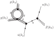
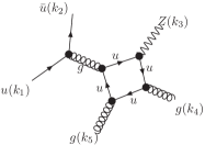
For the diagram generation both at tree level and one-loop level we employ the program QGRAF Nogueira:1991ex . This program already offers several ways of excluding unwanted diagrams, for example by requesting a certain number of propagators or vertices of a certain type or by specifying topological properties such as the presence of tadpoles or on-shell propagators. Although QGRAF is a very reliable and fast generator, we extend its possibilities by adding another level of analysing and filtering over diagrams by means of Python. This gives several advantages: first of all, the possibilities offered by QGRAF are not always sufficient to distinguish certain classes of diagrams (see examples in Fig. 1); secondly, QGRAF cannot handle the sign for diagrams with Majorana fermions in a reliable way; finally, in order to fully optimize the reduction, we want to classify and group diagrams according to the sets of their propagators.
Within our framework, QGRAF generates three sets of output files: an expression for each diagram to be processed with FORM Vermaseren:2000nd , Python code for drawing all diagrams, and Python code for computing the properties of each diagram. The information about the model for QGRAF is either read from the built-in Standard Model file or is generated from a user defined LanHEP Semenov:2010qt or Universal FeynRules Output (UFO) Degrande:2011ua file.
The Python program automatically performs several operations:
-
•
diagrams whose color factor turns out to be zero are dropped automatically;
-
•
the fermion flow is determined and used to compute an overall sign for each diagram, which is relevant in the presence of Majorana fermions;
-
•
the number of propagators containing the loop momentum, i.e. the loop size of the diagram, the tensor rank and the kinematic invariants of the associated loop integral are computed;
-
•
diagrams with an associated vanishing loop integral (see Fig. 1(a)) are detected and flagged for the diagram selection;
-
•
all propagators and vertices are classified for the diagram selection; diagrams containing massive quark self-energy insertions or closed massless quark loops are specially flagged.
Any one-loop diagram can be written in the form
| (1) |
where the numerator is a polynomial of tensor111 Index contractions in Eq. (2) are understood in -dimensional space. rank .
| (2) | ||||
| and the kinematic matrix is defined as | ||||
| (3) | ||||
All masses can be either real or complex. Important information about the integrals that will appear in the reduction of each one-loop diagram is contained in the tensor rank of the loop integral and its kinematic matrix .
We define a preorder relation on one-loop diagrams, such that if their associated matrices and are related by a finite (not necessarily unique) chain of transformations
| (4) |
where each transformation is one of the following:
-
•
the identity,
-
•
the simultaneous permutation of rows and columns,
-
•
the simultaneous deletion of the row and column with the same index, which corresponds to pinching the corresponding propagator in the diagram.
The relation “” can be read as “appears in the reduction of”. Our algorithm groups the one-loop diagrams of a process into subsets such that
-
•
form a partition of and
-
•
each cell contains a maximum element , such that .
The partitioning procedure provides an important gain in efficiency, because while carrying out the tensor reduction for the diagram , all other diagrams in the same cell are reduced with virtually no additional computational cost. The gain in efficiency can be observed when reducing the diagram using the OPP method Ossola:2006us and its implementations in CutTools Ossola:2007ax and Samurai Mastrolia:2010nb , as well as in classical tensor reduction methods as implemented e.g. in Golem95C Binoth:2008uq ; Cullen:2011kv , PJFRY Fleischer:2010sq and LoopTools Hahn:1998yk ; vanOldenborgh:1989wn .
In order to draw the diagrams, we first compute an ordering of the external legs which allows for a planar embedding of the graph. Such ordering can always be found for a tree or a one-loop graph since non-planar graphs only start to appear in diagrams with two or more loops. After the legs have been assigned to the vertices of a regular polygon, we use our own implementation of the algorithms described in Ohl:1995kr for fixing the coordinates of the remaining vertices; the algorithm has been extended to determine an appealing layout also for graphs containing tadpoles. Starting from these coordinates and using the package Axodraw Vermaseren:1994je , GoSam generates a LaTeX file that contains graphical representations of all diagrams.
2.3 Algebraic Processing
2.3.1 Color Algebra
In the models used by GoSam, we allow one unbroken gauge group to be treated implicitly; any additional gauge group, broken or unbroken, needs to be expanded explicitly. Any particle of the model may be charged under the group in the trivial, (anti-)fundamental or adjoint representation. Other representations are currently not implemented.
For a given process we project each Feynman diagram onto a color basis consisting of strings of generators and Kronecker deltas but no contractions of adjoint indices and no structure constants . Considering, for example, the process
GoSam finds the color basis
where and are the color parts of the quark and gluon wave functions respectively. The dimension of this color basis for external gluons and quark-antiquark pairs is given by Reiter:2009kb :
| (5) |
It should be noted that the color basis constructed in this way is not a basis in the mathematical sense, as one can find linear relations between the vectors once the number of external partons is large enough.
Any Feynman diagram can be reduced to the form
| (6) |
for the process specific color basis by applying the following set of relations:
| (7) | ||||
| (8) |
The same set of simplifications is used to compute the matrices and . The former is needed for squaring the matrix element, whereas the latter is used to provide color correlated Born matrix elements which we use for checking the IR poles of the virtual amplitude and also to provide the relevant information for parton showers like POWHEG Nason:2004rx ; Frixione:2007vw ; Alioli:2010xd . For the above example, GoSam obtains222In the actual code the results are given in terms of and only.
| (9) |
Similarly, the program computes the matrices for all pairs of partons and .
If denotes the tree-level matrix element of the process and we have
| (10) |
then the square of the tree level amplitude can be written as
| (11) |
For the interference term between leading and next-to-leading order we use a slightly different philosophy. First of all we note that it is sufficient to focus on a single group as defined in Section 2.2,
| (12) |
In order to reduce the complexity at the level of the reduction, we perform the contraction with the tree-level already at the integrand level,
| (13) |
where is formed by the sum over the corresponding coefficients of all diagrams .
2.3.2 Lorentz Algebra
In this Section we discuss the algorithms used by GoSam to transform the coefficients and , as defined in the previous section, such that the result is suitable for efficient numerical evaluation. One of the major goals is to split the -dimensional algebra () into strictly four-dimensional objects and symbols representing the higher-dimensional remainder.
In GoSam we have implemented the ’t Hooft-Veltman scheme (HV) and dimensional reduction (DRED). In both schemes all external vectors (momenta and polarisation vectors) are kept in four dimensions. Internal vectors, however, are kept in the -dimensional vector space. We adopt the conventions used in Cullen:2010jv , where denotes the four-dimensional projection of an in general -dimensional vector . The -dimensional orthogonal projection is denoted as . For the integration momentum we introduce in addition the symbol , such that
| (14) |
We also introduce suitable projectors by splitting the metric tensor
| (15) |
In the follwing, we describe the ’t Hooft algebra in detail. For DRED, the only differences are that the numerator algebra is performed in four dimensions for both external and internal vectors (i.e. ) and that in the very end all appearances of are replaced by .
Wave Functions and Propagators
GoSam contains a library of representations of wave functions and propagators up to spin two333Processes with particles of spin and spin 2 have not been tested extensively. Furthermore, these processes can lead to integrals where the rank is higher than the loop size, which at the moment are neither implemented in Samurai nor in Golem95C.. The exact form of the interaction vertices is taken from the model files.
The representation of all wave functions with non-trivial spin is based on massless spinors. Each massive external vector is replaced by its light-cone projection with respect to a lightlike reference vector ,
| (16) |
| , | , | |
|---|---|---|
| initial | ||
| final |
For spin particles we use the assignment of wave functions as shown in Table 1; here, we quote the definition of the massive spinors from Cullen:2010jv assuming the splitting of Eq. (16):
| (17a) | ||||||
| (17b) | ||||||
In order to preserve the condition that for any loop integral the tensor rank does not exceed the number of loop propagators we fix all gauge boson propagators to be in Feynman gauge. Their wave functions are constructed as Xu:1986xb
| (18) |
where in the massless case and according to Eq. (16) in the massive case. In the latter case the third polarisation is defined as
| (19) |
The wave functions and propagators for spin and spin 2 particles correspond to those in Kilian:2007gr .
Simplifications
Once all wave functions and propagators have been substituted by the above definitions and all vertices have been replaced by their corresponding expressions from the model file then all vector-like quantities and all metric tensors are split into their four-dimensional and their orthogonal part. As we use the ’t Hooft algebra, is defined as a purely four-dimensional object, . By applying the usual anti-commutation relations for Dirac matrices we can always separate the four-dimensional and -dimensional parts of Dirac traces, as we can use the fact that Reiter:2009kb ; Cullen:2010jv
| (20) |
The same logic applies to open spinor lines such as Cullen:2010jv
| (21) |
While the -dimensional traces are reduced completely to products of -dimensional metric tensors , the four-dimensional part is treated such that the number of terms in the resulting expression is kept as small as possible. Any spinor line or trace is broken up at any position where a light-like vector appears. Furthermore, Chisholm idenities are used to resolve Lorentz contractions between both Dirac traces and open spinor lines. If any traces remain we use the built-in trace algorithm of FORM Vermaseren:2000nd .
In the final result we can always avoid the explicit appearance of Levi-Civitá tensors, noticing that any such tensor is contracted with at least one light-like vector444Any external massive vector at this point has been replaced by a pair of light-like ones. Contractions between two Levi-Civitá symbols can be resolved to products of metric tensors. , and we can replace
| (22) |
Hence, the kinematic part of the numerator, at the end of our simplification algorithm, is expressed entirely in terms of:
-
•
spinor products of the form , or ,
-
•
dot products or ,
-
•
constants of the Lagrangian such as masses, widths and coupling constants,
-
•
the symbols and .
Treatment of rational terms
In our representation for the numerator of one-loop diagrams, terms containing the symbols or can lead to a so-called term Ossola:2008xq , which contributes to the rational part of the amplitude. In general, there are two ways of splitting the numerator function:
| (23a) | ||||
| or, alternatively, | ||||
| (23b) | ||||
It should be noted that in Eq. (23) the terms and do not arise in DRED, where only terms containing contribute to . Instead of relying on the construction of from specialized Feynman rules Draggiotis:2009yb ; Garzelli:2009is ; Garzelli:2010qm ; Garzelli:2010fq , we generate the part along with all other contributions without the need to separate the different parts. For efficiency reasons, however, we provide an implicit and an explicit construction of the terms.
The implicit construction uses the splitting of Eq. (23) and treats all three numerator functions on equal grounds. Each of the three terms is reduced separately in a numerical reduction and the Laurent series of the three results are added up taking into account the powers of .
The explicit construction of is based on the assumption that each term in in Eq. (23b) contains at least one power of or . The expressions for those integrals are relatively simple and known explicitly. Hence, the part of the amplitude which originates from is computed analytically whereas the purely four-dimensional part is passed to the numerical reduction.
2.4 Code Generation
2.4.1 Abbreviation System
To prepare the numerator functions of the one-loop diagrams for their numerical evaluation, we separate the symbol and dot products involving the momentum from all other factors. All subexpressions which do not depend on either or are substituted by abbreviation symbols, which are evaluated only once per phase space point. Each of the two parts is then processed using haggies Reiter:2009ts , which generates optimized Fortran code for their numerical evaluation. For each diagram we generate an interface to Samurai Mastrolia:2010nb , Golem95C Cullen:2011kv and/or PJFRY Fleischer:2010sq . The two latter codes are interfaced using tensorial reconstruction at the integrand level Heinrich:2010ax .
2.4.2 Reduction Strategies
In the implementation of GoSam, great emphasis has been put on maintaining flexibility with respect to the reduction algorithm that the user decides to use. On the one hand, this is important because the best choice of the reduction method in terms of speed and numerical stability can strongly depend on the specific process. On the other hand, we tried to keep the code flexible to allow further extensions to new reduction libraries, such that GoSam can be used as a laboratory for interfacing future methods with a realistic environment.
Our standard choice for the reduction is Samurai, which provides a very fast and stable reduction in a large part of the phase space. Furthermore, Samurai reports to the client code if the quality of the reconstruction of the numerator suffices the numerical requirements (for details we refer to Mastrolia:2010nb ). In GoSam we use this information to trigger an alternative reduction with either Golem95C Cullen:2011kv or PJFRY Fleischer:2010sq whenever these reconstruction tests fail, as shown in Fig. 2. The reduction algorithms implemented in these libraries extend to phase space regions of small Gram determinants and therefore cover most cases in which on-shell methods cannot operate sufficiently well. This combination of on-shell techniques and traditional tensor reduction is achieved using tensorial reconstruction at the integrand level Heinrich:2010ax , which also provides the possibility of running on-shell methods with a reconstructed numerator. In addition to solving the problem of numerical instabilities, in some cases this option can reduce the computational cost of the reduction. Since the reconstructed numerator is typically of a form where kinematics and loop momentum dependence are already separated , the use of a reconstructed numerator tends to be faster than the original procedure, in particular in cases with a large number of legs and low rank.
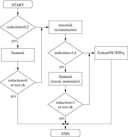
The flowchart in Fig. 2 summarizes all possible reduction strategies which are currently implemented. The strategy in use is selected by assigning the variable reduction_interoperation in the generated Fortran code. The availability of the branches is determined during code generation by activating (at least one of) the extensions (samurai, golem95, pjfry) in the input card. Switching between active branches is possible at run time. In detail, the possible choices for the variable reduction_interoperation are the following:
- 0
-
the numerators of the one-loop diagrams are reduced by Samurai, no rescue system is used in case the reconstruction test fails;
- 1
-
the tensor coefficients of the numerators are reconstructed using the tensorial reconstruction at the integrand level, the numerator is expressed in terms of tensor integral form factors which are evaluated using Golem95C;
- 2
-
the numerators are reduced by Samurai; whenever the reconstruction test fails, numerators are reduced using the option 1 as a backup method;
- 3
-
tensorial reconstruction is used to compute the tensor coefficients; Samurai is employed for the reduction of the reconstructed numerator, no rescue system is used;
- 4
-
as in option 3, Samurai is used to reduce the reconstructed numerator, Golem95C is used as backup option;
- 11
-
same as 1 but PJFRY is used instead of Golem95C;
- 12
-
same as 2 but PJFRY is used instead of Golem95C;
- 14
-
same as 4 but PJFRY is used instead of Golem95C.
It is difficult to make a statement about the “optimal” reduction method because this depends on the process under consideration. For multi-leg processes, e.g. production, we found that Samurai is clearly superior to tensor reduction in what concerns timings and size of the code. Concerning points which need a special treatment, we did not make extensive studies using traditional tensor reduction only, but one can certainly say that the combination of Samurai and tensorial reconstruction seems to be optimal in what concerns the avoidance of numerical instabilities due to inverse Gram determinants.
2.5 Conventions of the Amplitudes
In this section we briefly discuss the conventions chosen for the results returned by GoSam. Depending on the actual setup for a given process, in particular if an imported model file is used, conventions may be slightly different. Here we restrict the discussion to the case where the user wants to compute QCD corrections to a process and in the setup files he has put . In this case, the tree-level matrix element squared can be written as
| (24) |
The fully renormalised matrix element at one-loop level, i.e. the interference term between tree-level and one-loop, can be written as
| (25) |
A call to the subroutine samplitude returns an array consisting of the four numbers in this order. The average over initial state colours and helicities is included in the default setup. In cases where the process is loop induced, i.e. the tree level amplitude is absent, the program returns the values for where a factor
has been pulled out.
After all UV-renormalisation contributions have been taken into account correctly, only IR-singularities remain, which can be computed using the routine ir_subtractions. This routine returns a vector of length two, containing the coefficients of the single and the double pole, which should be equal to and therefore can be used as a check of the result.
Ultraviolet Renormalisation in QCD
For UV-renormalisation we use the scheme for the gluon and all massless quarks, whereas a subtraction at zero momentum is chosen for massive quarks Nason:1987xz . Currently, counterterms are only provided for QCD corrections. In the case of electroweak corrections only unrenormalised results can be produced automatically.
For computations involving loop propagators for massive fermions, we introduced the automatic generation of a mass counter term needed for the on-shell renormalisation of the massive particle. Here, we exploit the fact that such a counter term is strictly related to the massive fermion self energy bubble diagrams (see Fig. 3).

As described in Section 2.2, the program GoSam analyzes all generated diagrams. In that step also self-energy insertions of massive quarks are detected, where we make the replacement
| (26) |
The symbol is one in the ’t Hooft Veltman scheme and zero in DRED.
Performing the integral, contracting the expression with the QCD vertices at both sides and multiplying the missing factor of we retrieve the expression for the mass counter-term,
| (27) |
Furthermore, the renormalisation of leads to a term of the form
| (28) |
with , being the number of light quark flavours, the number of heavy flavours, and is the power of the coupling in the Born amplitude as defined in Eq. (24). The last term of Eq. (28) provides the finite renormalisation needed to compensate the scheme dependence of ,
| (29) |
A further contribution consists of the wave-function renormalisation of massive external quark lines. If we denote the set of external massive quark lines by we obtain
| (30) |
Finally, also the wave function of the gluon receives a contribution from the presence of heavy quarks in closed fermion loops. If is the number of external gluon lines, this contribution can be written as
| (31) |
At the level of the generated Fortran code the presence of these
contributions can be controlled by a set of variables defined in the
module config.f90. The variable renormalisation
can be set to 0, 1, or 2.
If renormalisation=0, none of the counterterms ar present. If
renormalisation=2 only
is included,
which is the counterterm stemming from all terms of the type of Eq. (27)
contributing to the amplitude.
In the case where renormalisation=1 a more fine-grained control
over the counterterms is possible.
- •
- •
-
renorm_beta: if set to false, the counterterm is set to zero.
- •
-
renorm_mqwf: if set to false, the counterterm is set to zero.
- •
-
renorm_mqse: if set to false, the counterterm is set to zero.
- •
-
renorm_decoupling if set to false, the counterterm is set to zero.
The default settings for renormalisation=1 are true for all the renorm options listed above.
Finite Renormalisation of in QCD
In the ’t Hooft Veltman scheme, a finite renormalisation term for is required beyond tree level. The relevant terms are generated only if fr5 is added in the input card to the list of extensions before code generation. Currently, the automatic generation of this finite contribution is not performed if model files different from the built-in model files are used. In agreement with Harris:2002md and Weinzierl:1999xb we replace the axial component at each vertex,
| (32) | ||||
| with | ||||
| (33) | ||||
Once it is generated, this contribution can be switched on and off at run-time through the variable renorm_gamma5, which is defined in the module config.f90.
Conversion between the Schemes
In GoSam we have implemented two different schemes, the ’t Hooft Veltman scheme and dimensional reduction. By default, the former is used, while the latter can be activated by adding the extension dred. If a QCD computation has been done in dimensional reduction the result can be converted back to the ’t Hooft Veltman scheme by adding a contribution for each external massless parton,
| (34) |
with and . This conversion can be switched on by setting convert_to_cdr to true in the module config.f90. At one-loop level, the ’t Hooft Veltman scheme and conventional dimensional regularisation (CDR) are equivalent in the sense that for all partons.
3 Requirements and Installation
3.1 Requirements
The program GoSam is designed to run in any modern Linux/Unix environment; we expect that Python (), Java () and Make are installed on the system. Furthermore, a Fortran 95 compiler is required in order to compile the generated code. Some Fortran 2003 features are used if one wants to make use of the Les Houches interface Binoth:2010xt . We have tried all examples using gfortran versions 4.1 and 4.5.
On top of a standard Linux environment, the programs FORM Vermaseren:2000nd , version (newer than Aug.11, 2010) and QGRAF Nogueira:1991ex need to be installed on the system. Whereas spinney Cullen:2010jv and haggies Reiter:2009ts are part of GoSam and are not required to be installed separately, at least one of the libraries Samurai Mastrolia:2010nb and Golem95C Cullen:2011kv needs to be present at compile time of the generated code. Optionally, PJFRY Fleischer:2010sq can be used on top of Golem95C.
3.2 Download and Installation
QGRAF
The program can be downloaded as Fortran source code from
\urlhttp://cfif.ist.utl.pt/ paulo/qgraf.html .
After unpacking the tar-ball, a single Fortran 77 file needs to be compiled.
FORM
The program is available at
\urlhttp://www.nikhef.nl/ form/
both as a compiled binary for many platforms and as a tar-ball. The build process, if built from the source files, is controlled by Autotools.
Samurai and Golem95C
These libraries are available as tar-balls and from subversion repositories at
\urlhttp://projects.hepforge.org/samurai/
and
\urlhttp://projects.hepforge.org/golem/95/
respectively. For the user’s convenience we have prepared a package containing Samurai and Golem95C together with the integral libraries OneLOop vanHameren:2010cp , QCDLoop Ellis:2007qk and FF vanOldenborgh:1989wn . The package gosam-contrib-1.0.tar.gz containing all these libraries is available for download from:
\urlhttp://projects.hepforge.org/gosam/
GoSam
The user can download the code either as a tar-ball or from the subversion repository at
\urlhttp://projects.hepforge.org/gosam/ .
The build process and installation of GoSam is controlled by Python Distutils, while the build process for the libraries Samurai and Golem95C is controlled by Autotools.
Therefore the installation proceeds in two steps:
-
1.
For all components which use Autotools, the following sequence of commands installs them under the user defined directory MYPATH.
If the configure script is not present, the user needs to run sh ./autogen.sh first.
-
2.
For GoSam which is built using Distutils, the user needs to run
If MYPATH is different from the system default (e.g. /usr/bin), the environment variables PATH, LD_LIBRARY_PATH and PYTHONPATH might have to be set accordingly. For more details we direct the user to the GoSam reference manual and to the documentation of the beforementioned programs.
4 Using GoSam
4.1 Setting up a simple Process
GoSam is a very flexible program and comes with a wide range of configuration options. Not all of these options are relevant for simple processes and often the user can leave most of the settings at their default values. In order to generate the code for a process, one needs to prepare an input file, which will be called process card in the following, which contains
-
•
process specific information, such as a list of initial and final state particles, their helicities (optional) and the order of the coupling constants;
-
•
scheme specific information and approximations, such as the regularisation and renormalisation schemes, the underlying model, masses and widths which are set to zero, the selection of subsets of diagrams; the latter might be process dependent;
-
•
system specific information, such as paths to programs and libraries or compiler options;
-
•
optional information for optimisations which control the code generation.
In the following we explain how to set up the required files for the process . The example computes the QCD corrections for the initial state, where and massless quarks are assumed. For our example, we follow an approach where we keep the different types of information in separate files – process.rc, scheme.rc and system.rc – and use GoSam to produce a process card for this process based on these files. This is not required — one could also produce and edit the process card directly — it is however more convenient to store system specific information into a separate, re-usable file, and it makes the code generation more transparent.
Process specific information
The following listing contains the information which is specific to the process. The syntax of process cards requires that no blank character is left between the equals sign and the property name. Commentary can be added to any line, marked by the ‘#’ character. Line continuation is achieved using a backslash at the end of a line.555The line numbers are just for reference and should not be included in the actual files.
The first line defines the (relative) path to the directory where the process files will be generated. GoSam expects that this directory has already been created. Lines 2 and 3 define the initial and final state of the process in terms of field names, which are defined in the model file. Besides the field names one can also use PDG codes Yost:1988ke ; Caso:1998tx instead. Hence, the following lines would be equivalent to lines 2 and 3 in Listing 1:
Line 4 describes the helicity amplitudes which should be generated. If no helicities are specified, the program defaults to the generation of all possible helicity configurations, some of which may turn out to be zero. The different helicity amplitudes are separated by commas; within one helicity amplitude there is one character (usually ‘+’, ‘-’ and ‘0’) per external particle from the left to the right. In the above example for the reaction
we have the following assignments:
| Helicity | |||||
|---|---|---|---|---|---|
| 0 | + | - | + | - | + |
| 1 | + | - | - | - | + |
| 2 | - | + | + | - | + |
| 3 | - | + | - | - | + |
With the above value for helicities we generate all non-vanishing helicities for the partons but keep the lepton helicities fixed. In more complicated examples this way of listing all helicities explicitly can be very tedious. Therefore, we introduced the option to generate sets of helicities using square brackets. For example, if the gluon helicity is replaced by [+-], the bracket is expanded automatically to take the values +,-.
A further syntactical reduction can be achieved for the quarks. The current expansion of a square bracket and its opposite value can be assigned to a pair of variables as in [xy=+-]. If the bracket expands to ‘+’ then x is assigned ‘+’ and y is assigned the opposite sign, i.e. ‘-’. If the bracket expands to ‘-’ the assignments are x=- and y=+. Hence, the helicity states of a massless quark anti-quark pair are generated by [qQ=+-]Q, and the selection of helicities in our example can be abbreviated to
which is equivalent to the version of this line in Listing 1.
Finally, the order (power) of the coupling constants has to be specified. Line 5 contains a keyword for the type of coupling (QCD or QED), the order of this coupling constant in the unsquared tree level amplitude (in our example: 1) and the order of the coupling constant in the unsquared one-loop amplitude (in our example: 3). One can also use GoSam to generate the tree level only, by giving only the power of the tree level amplitude:
Conversely, GoSam will generate the virtual amplitude squared for processes where no tree level is present if the tree level order is replaced by the keyword NONE.
Up to now, the file would generate all 8 tree level and 180 one-loop diagrams contributing to the process , regardless of the intermediate states. Nevertheless, what we intended to generate were only those diagrams where the electron pair comes from the decay of a . GoSam offers two ways of achieving this diagram selection, either by passing a condition to QGRAF or by applying a filter written in Python. The first option would be specified by the option qgraf.verbatim, which copies the argument of the option to the QGRAF input file in verbatim. The following filter demands the appearance of exactly one -propagator, leaving us with 2 tree-level and 45 one-loop diagrams:
The alternative solution is the application of a Python filter using the options filter.lo for tree level and filter.nlo for one-loop diagrams. The current example requires the two lines
Scheme specific information
For our example we put all scheme specific definitions in the file scheme.rc. It contains the choice of a suitable regularisation scheme and fixes what types of UV counterterms are included in the final result.
In Listing 2, line 1 selects dimensional reduction as a regularisation scheme. If dred is not specified in the list of extensions, GoSam works in the ’t Hooft Veltman scheme by default. Line 2 removes all on-shell bubbles on external legs. This is, on the one hand, required to be consistent with the renormalisation scheme. On the other hand, those diagrams would lead to zero denominators at the algebraic level. In line 3 all light quark masses, the mass of the electron and the width of the top quark are set to zero. Further, as a convention rather than a scheme, the strong coupling is set to one in line 4, which means that will not occur in the algebraic expressions, assuming that the user will multiply the final result by his desired value for the strong coupling. If the option one=gs is not used, the default value contained in the file common/model.f90 will be used. This default value of course can be changed by the user.
System specific information
In order to adapt the code generation to the system environment, GoSam needs to find a way of determining all relevant paths and options for the programs and libraries used during generation, compilation and linking of the code. Those settings are fixed in the file system.rc in our example.666In this example we assume that the user has defined an environment variable PREFIX.
Generating the Code
After having prepared the input files correctly we need to collect the information distributed over the three files process.rc, scheme.rc and system.rc in one input file, which we will call gosam.in here. The corresponding command is:
The generated file can be processed with gosam.py directly but requires the process directory to be present.
All further steps are controlled by the generated make files; in order to generate and compile all files relevant for the matrix element one needs to invoke
The generated code can be tested with the program matrix/test.f90. The following sequence of commands will compile and run the example program.
The last lines of the program output should look as follows777The actual numbers depend on the random number generator of the system because the phase space point is generated randomly; however, the pole parts should agree between the matrix element and the infrared insertion operator given that the matrix element is fully renormalised.
The printed numbers are, in this order, , , , and the pole parts calculated from the infrared insertion operator Catani:1996vz ; Catani:2000ef .
One can generate a visual representation of all generated diagrams using the command
which generates the file doc/process.ps using a Python implementation of the algorithm described in Ohl:1995kr and the LaTeX package AXODRAW Vermaseren:1994je .
4.1.1 Further Options
GoSam provides a range of options which influence the code generation, the compilation and the numerical evaluation of the amplitude. Giving an exhaustive list of all options would be far beyond the scope of this article and the interested user is referred to the reference manual. Nonetheless, we would like to point out some of GoSam’s capabilities by presenting the corresponding options.
Generating the Term
When setting up a process the user can specify if and how the term of the amplitude should be generated by setting the variable r2 in the setup file.
Possible options for r2 are implicit, which is the default, explicit, off and only. The keyword implicit means that the term is generated along with the four-dimensional numerator as a function in terms of , and and is reduced at runtime by sampling different values for . This is the slowest but also the most general option. Using the keyword explicit carries out the reduction of terms containing or during code generation (see Appendix B). The keyword off puts the term to zero which is useful if the user wants to provide his own calculation for these terms. Conversely, using r2=only discards everything but the term (reducing it as in the case explicit) and puts GoSam in the position of providing terms for external codes which work entirely in four dimensions.
Diagram Selection
GoSam offers a two-fold way of selecting and discarding diagrams. One can either influence the way QGRAF generates diagrams or apply filters to the diagrams after they have been generated by QGRAF or combine the two methods. Let us assume that in the above example we want to remove the third generation of quarks completely. Hence, all closed quark loops would be massless and therefore the second generation is just an exact copy of the first one. We can therefore restrict the generation of closed quark loops to up and down quarks. GoSam has a filter precisely for this purpose, which takes the field names of the flavours to be generated as arguments.
This filter can be combined with the already existing filter selecting only diagrams containing a -propagator using the AND function:
A further feature of the code generated by GoSam is the possibility of selecting diagrams at runtime. For example, we would like to distinguish at runtime three different gauge invariant sets of diagrams at one-loop level:
-
1.
diagrams with a closed quark loop where the is attached to the loop;
-
2.
diagrams with a closed quark loop where the is emitted from the external quark line;
-
3.
diagrams without a closed quark loop.
In order to provide the code for a diagram selection at runtime one simply replaces the above filter by a list of filters as follows
The two new filters in use are NF which selects closed quark loops only and LOOPVERTICES which counts the number of vertices attached to the loop with the given sets of fields running through the vertex (where _ replaces any field). In the Fortran files one can access the diagram selection through the routine update_flags. The three selection criteria are stored in a derived data type virt_flags which has fields eval_0, …, eval_2, in general ranging from zero to the length of the list given in filter.nlo.
Additional Extensions
Some of GoSam’s functionality is available through the extensions variable. On top of the already presented options for selecting a regularisation scheme (by adding the option dred) or for activating interfaces to several different reduction libraries (samurai, golem95, pjfry) the user can also add the following options:
- fr5
-
adds and activates the relevant code for the computation of the finite renormalisation of required in the ’t Hooft Veltman scheme as described in Eq. (32).
- powhegbox
-
generates routines for the computation of the color and spin correlated Born matrix elements as required by POWHEG Alioli:2010xd .
- autotools
-
uses make files which use Autoconf and Automake for compilation of the matrix element.
- gaugecheck
-
replaces the polarisation vectors of external vector fields by
(35) where the variable defaults to zero and is accessible in the Fortran code through the symbol gaugeiz.
4.2 Interfacing the code
The matrix element code generated by GoSam provides several routines to transparently access partial or full results of the amplitude calculation. Here, we only present a minimal set of routines which can be used to obtain the set of coefficients for a given scale and a given set of external momenta. The routines, which can be accessed through the modules matrix888If a process name was given all modules are prefixed by the name, e.g. if process_name=pr01, the module matrix would be renamed into pr01_matrix. are defined as follows:
- initgolem
-
This subroutine must be called once before the first matrix element evaluation. It initializes all dependent model parameters and calls the initialisation routines of the reduction libraries.
interfacesubroutine initgolem(init_libs)use config, only: kilogical, optional, && intent(in) :: init_libsend subroutineend interfaceThe optional argument init_libs can usually be omitted. It should be used only when several initialisation calls become necessary, but the reduction libraries and loop libraries should be initialized only once. All model parameters are accessible as global variables in the module model and should be modified (if at all) before calling initgolem.
- samplitude
-
This subroutine starts the actual calculation of the amplitude for a given phase space point.
interfacesubroutine samplitude && (vecs,scale2,amp,ok,h)use config, only: kiuse kinematics, only: num_legsreal(ki), dimension(num_legs,4),&& intent(in) :: vecsdouble precision, && intent(in) :: scale2double precision, && intent(out) :: amplogical, optional, && intent(out) :: okinteger, optional, && intent(in) :: hend subroutineend interfaceThe first mandatory arguments of this routine are the external momenta vecs, where vecs(i,:) contains the momentum of the -th particle as a vector , and we use in-out kinematics, i.e. . Maximal numerical stability is achieved if the beam axis is chosen along the -axis. The second argument, , is the square of the renormalisation scale. As a third argument the routine expects a vector which accepts the result in the format with the coefficents being defined in Eqs. (24) and (25). The optional argument ok may be used in order to report the outcome of the reconstruction tests in samurai if no rescue method has been chosen (see Section 2.4.2). The last argument allows one to select a single helicity subamplitude; the index h runs from zero to the number of helicities minus one. The labeling of the helicities is documented for each process in the file doc/process.ps.
- exitgolem
-
This routine should be called once after the last amplitude evaluation in the program. It closes all open log files and gracefully terminates the reduction and loop libraries.
interfacesubroutine exitgolem(exit_libs)use config, only: kilogical, optional,& intent(in) :: exit_libsend subroutineend interfaceThe optional argument exit_libs should only be set if multiple calls to this routine (e.g. for different matrix elements) are necessary and the dependent libraries should be terminated only once.
A small program which computes the amplitude for a set of phase space points is automatically generated with the amplitude code in the file test.f90 in the subdirectory matrix. The script config.sh in the process directory returns suitable compilation and linking options for the generated matrix element code.
4.3 Using the BLHA Interface
The so-called Binoth Les Houches Accord (BLHA) Binoth:2010xt defines an interface for a standardized communication between one-loop programs (OLP) and Monte Carlo (MC) tools. The communication between the two sides is split into two main phases: an initialisation phase and a runtime phase. During initialisation the two programs establish an agreement by exchanging a set of files and typically initiate the code generation. The OLP runtime code is then linked to the MC program and, during the runtime phase, called through a well-defined set of routines providing NLO results for the phase space points generated by the MC. According to this standard, it is the responsibility of the MC program to provide results for the Born matrix element, for the real emission and for a suitable set of infrared subtraction terms. A schematic overview on this procedure is shown in Fig. 4.

GoSam can act as an OLP in the framework of the BLHA. In the simplest case, the MC writes an order file — in this example it is called olp_order.lh — and invokes the script gosam.py as follows:
Further, GoSam specific options can be passed either in a file or directly at the command line. One can, for example, use autotools for the compilation by modifying the above line as follows.
The contract file is given the extension .olc by default and would be olp_order.olc in this example. Alternatively, the name can be altered using the -o option.
If successful, the invocation of gosam.py generates a set of files which can be compiled as before with a generated make file. The BLHA routines are defined in the Fortran module olp_module but can also be accessed from C programs999A header file is provided in olp.h.. The routines OLP_Start and OLP_EvalSubProcess are defined exactly as in the BLHA proposal Binoth:2010xt . For convenience, we extended the interface by the functions OLP_Finalize(), which terminates all reduction libraries, and OLP_Option(char*,int*), which can be used to pass non-standard options at runtime. For example, a valid call in C to adjust the Higgs mass would be
A value of one in ierr indicates that the setting was successful. A value of zero indicates an error.
4.4 Using External Model Files
With a few modifications in the process description files, GoSam can immediately make use of model files generated by either FeynRules Christensen:2008py in the UFO format Degrande:2011ua or by LanHEP Semenov:2010qt . In both cases, the following limitations and differences with respect to the default model files, sm and smdiag, apply:
-
•
As usual, particles can be specified by their PDG code. The field names, as used by QGRAF, are part and anti for the particles with the PDG code and respectively. For example, the and the boson would be called part24 and anti24.
-
•
All model parameters are prefixed by the letters mdl in order to avoid name clashes with existing variable names in the matrix element code.
-
•
The variable model.options and the extension fr5 are not guaranteed to work with models other than the built-in models.
Importing models in the UFO format
A model description in the UFO format consists of a Python package stored in a directory. In order to import the model into GoSam one needs to set the model variable in the input card to specify the keyword FeynRules in front of the directory name, where we assume that the model description is in the directory $HOME/models/MSSM_UFO.
Importing models in the LanHEP format
LanHEP model descriptions consist of a set of plain text files in the same directory with a common numbering (such as func4.mdl, lgrng4.mdl, prtcls4.mdl, vars4.mdl). A LanHEP model can be loaded by specifying the path and the common number in the model variable. Assuming the files are situated in the directory $HOME/models/MSSM_LHEP one would set the variable as follows.
Details about the allowed names for the table columns are described in the GoSam reference manual. Precompiled MSSM_UFO and MSSM_LHEP files can also be found in the subdirectory examples/model.
5 Sample Calculations and Benchmarks
The codes produced by GoSam have been tested on several processes. In this section we describe some examples of applications. Additional results, whose corresponding code is also included in the official distribution of the program, will be reported in Appendix B.
5.1 \texorpdfstringp p –¿ W j with SHERPA
In Section 4.3 the BLHA interface of GoSam was presented. This interface allows one to link the program to a Monte Carlo event generator, which is, in general, responsible for supplying the missing ingredients for a complete NLO calculation of a physical cross section. Among the different general purpose Monte Carlo event generators, SHERPAGleisberg:2008ta is one of those which offers these tools: computing the LO cross section, the real corrections with both the subtraction terms and the corresponding integrated counterparts Krauss:2001iv ; Gleisberg:2007md ; Schonherr:2008av . Furthermore, SHERPA offers the possibility to match a NLO calculation with a parton shower Hoche:2010pf ; Hoeche:2011fd . Using the BLHA interface, we linked GoSam with SHERPA to compute the physical cross section for jet at NLO.
The first steps to perform this linking is to write a SHERPA input card for the desired process. Instructions and many examples on how to write this can be found in the on-line manual Sherpa1.3.1:online . Running the code for the first time will produce an order file OLE_order.lh which contains all the necessary information for GoSam, to produce the desired code for the loop part of the process. This includes a list of all partonic subprocesses needed. In parallel to the production of the needed SHERPA libraries with the provided script, one can at this point run the gosam.py command with the flag --olp and the correct path to the order file as explained in Section 4.3. Further options may be specified. Among them it is useful to have a second, GoSam-specific, input card with all the important GoSam options. Since, at the end, SHERPA needs to be linked to a dynamic library, it is convenient to run GoSam with the autotools extension, which allows the direct creation of both static and dynamic libraries, together with the test routine test. The gosam.py script creates all the files needed for interfacing GoSam with the Monte Carlo event generator together with the code for the one-loop computation of all needed subprocesses, and a makefile to run them. The different parton-level subprocesses are contained in different subdirectories. At this point the user simply has to run the makefile to generate and compile the code. Once the one-loop part of the code is ready, the produced shared library must be added to the list of needed libraries in the SHERPA input card as follows.
With this operation the generation of the code is completed. The evaluation of the process and the physical analysis can then be performed at the user’s discretion following the advice given in the SHERPA on-line documentation Sherpa1.3.1:online .
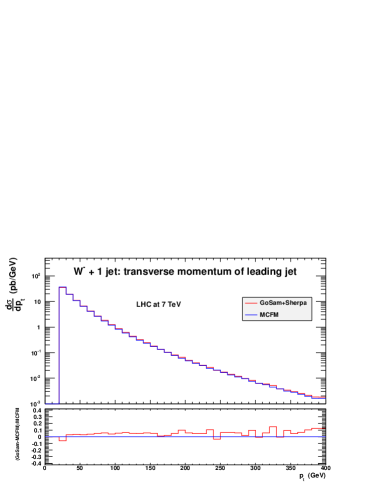
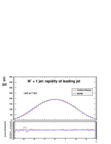
We tested the BLHA interface by computing jet and producing distributions for several typical observables. In Figs. 5(a) and 5(b) the inclusive transverse momentum and rapidity of the jets is shown. These distributions were compared with similar ones produced using the program MCFM Campbell:1999ah ; Campbell:2011bn , and perfect agreement was found.
5.2 \texorpdfstringp p –¿ W j, EW Corrections
As a first example of an electroweak calculation, we computed the virtual one-loop corrections to . A complete analytical calculation for this process was presented in Ref. Kuhn:2007cv .
| 500 | 0 | 0 | 500 | |
| 500 | 0 | 0 | 500 | |
| 503.23360778049988 | 110.20691318538486 | 441.95397288433196 | -198.26237811718670 | |
| 496.76639221950012 | -110.20691318538488 | -441.95397288433202 | 198.26237811718664 |
| parameters | |||
|---|---|---|---|
| 91.1876 | 80.419 | ||
| 0.88156596117995394232 | |||
For the kinematic point given in Tab. 2 and the above parameters we obtain the following result:
| result | ||
|---|---|---|
| 2.812364835883295 | ||
| unren. | -94.52525523327047 | |
| unren. | 17.84240236996827 | |
| unren. | -0.5555555555555560 | |
| renormalized | ||
| GoSam | Eqs.(67,70) of Ref. Kuhn:2007cv | |
| 4.743825167813529 | 4.7438251678146885 | |
| -0.5555555555555560 | -0.5555555555555555 | |
The poles have been renormalized using Eqs.(49)-(64) in Sections 3.3 and 3.4 of Kuhn:2007cv . Our result is agreement with Eqs.(67),(70) of Ref. Kuhn:2007cv and with Ref. Gehrmann:2010ry for the infrared divergences that remain after renormalisation.
5.3 \texorpdfstringphoton photon –¿ photon photon
The process in the Standard Model first arises at the one-loop order, and proceeds through a closed loop of fermions and bosons. Of the 16 helicity amplitudes contributing to it, only three are independent and their analytic expressions can be found in Gounaris:1999gh . The pure QED contribution, involving a fermion loop, is contained in samurai-1.0 Mastrolia:2010nb and will not be repeated here. Instead, we show the results of the -loop contribution to the independent helicity amplitudes, as an example of EW corrections that can be handled with GoSam.
| 500 | 0 | 0 | 500 | |
| 500 | 0 | 0 | -500 | |
| 500 | 436.6186300198938284 | -59.1784256571505765 | 236.3516148798047425 | |
| 500 | -436.6186300198938284 | 59.1784256571505765 | -236.3516148798047425 |
| parameters | |||
|---|---|---|---|
| 1000 | |||
| 80.376 | 1 | ||
With the above parameters and the kinematics of Tab. 3 we obtain the following results.
| result (EW) | ||
|---|---|---|
| GoSam(dred) | Refs.Gounaris:1999gh | |
| 12.02541904626610 | 12.025419045962 | |
| 7.380406043429961 | 7.3804060437434 | |
| 982.7804939723322 | 982.78049397093 | |
5.4 \texorpdfstringp p –¿ chi^0_1 chi^0_1 in the MSSM
As an example for the usage of GoSam with a model file different from the Standard Model we calculated the QCD corrections to neutralino pair production in the MSSM. The model file has been imported via the interface UFO (Universal FeynRules Output) Degrande:2011ua which facilitates the import of Feynman rules generated by FeynRules Christensen:2008py to programs generating one-loop amplitudes. To import such files within the GoSam setup, all the user has to do is to give the path to the corresponding model file in the input card.
For this example, we combined the one-loop amplitude with the real radiation corrections to obtain results for differential cross sections. A calculation of neutralino pair production for the LHC presenting total cross sections at NLO is given in Beenakker:1999xh .
For the infrared subtraction terms the program MadDipole Frederix:2008hu ; Frederix:2010cj is used, the real emission part is calculated using MadGraph/MadEvent Alwall:2007st . The virtual matrix element is renormalized in the scheme, while massive particles are treated in the on-shell scheme. The renormalisation terms specific to the massive MSSM particles have been added manually.
In Fig. 6 we show the differential cross section for the invariant mass, where we employed a jet veto to suppress large contributions from the channel which opens up at order , but for large belongs to the distinct process of neutralino pair plus one hard jet production at leading order. We used massless quark flavours and the MSTW08 Martin:2009iq parton distribution functions. For the SUSY parameters we use the modified benchmarks point SPS1amod suggested in Feigl:2011sw , and we use TeV.

For reference, we also give the result for the unrenormalised amplitude at one specific phase space point for in the DRED scheme, using the following parameters and momenta:
| 1000 | 0 | 0 | 1000 | |
| 1000 | 0 | 0 | -1000 | |
| 1000 | 42.3752677206678996 | 115.0009952646289548 | 987.7401101322898285 | |
| 1000 | -42.3752677206678996 | -115.0009952646289548 | -987.7401101322898285 |
| parameters | |||
|---|---|---|---|
| 91.1876 | 0 | ||
| 79.829013 | |||
| 1 | |||
| 1 | 127.934 | ||
| 96.6880686 | 607.713704 | ||
| 561.119014 | 549.259265 | ||
| 110.899057 | 399.960116 | ||
All widths have been set to zero; for further settings we refer to the model parameter files contained in the subdirectory examples/model/MSSM_UFO. We have checked that the pole terms of the renormalised amplitude cancel with the infrared poles from MadDipole. For the phase space point given in Tab. 4 we obtain the following numbers.
| GoSam result | |
|---|---|
| 0.8680577964243597 | |
| -31.9136615197871 | |
| 13.4374663711899 | |
| 2.6666666666667 | |
5.5 \texorpdfstringe+ e- –¿ e+ e- photon in QED
As an example of a QED calculation, we compared the virtual QED corrections for the process with the results provided in Actis:2009uq . The results compared in the table are the bare unrenormalised amplitudes in the ’t Hooft Veltman scheme. No counterterms or subtraction terms have been added to the result.
| (in) | 0.5 | 0 | 0.4999997388800458 | 0 |
|---|---|---|---|---|
| (in) | 0.5 | 0 | -0.4999997388800458 | 0 |
| (out) | 0.1780937847558600 | −0.1279164180985903 | 0.05006809884093004 | −0.1133477415216646 |
| (out) | 0.3563944406457374 | −0.02860530642319879 | −0.1832142729949070 | −0.3043534176228102 |
| 0.4655117745984024 | 0.1565217245217891 | 0.1331461741539769 | 0.4177011591444748 |
| parameters | |||
|---|---|---|---|
| 1.0 | |||
Using the parameters given above and the kinematics of Tab. 5 we obtain the following results.
| result | ||
|---|---|---|
| GoSam | Ref. Actis:2009uq | |
5.6 \texorpdfstringpp –¿ t t-bar H
This process has been compared with the results given in Hirschi:2011pa . The partonic subprocesses and where computed both in the ’t Hooft Veltman scheme and in dimensional reduction and the fully renormalised results were successfully compared as an internal consistency check. Apart from wave function renormalisation and mass counterterms, Yukawa coupling renormalisation is also needed here. Yukawa coupling counterterms are in this case equal to the wave function counterterms. The Yukawa top mass is set equal to its pole mass.
| parameters | |||
|---|---|---|---|
| 500.0 | 5 | ||
| 1 | |||
| 172.6 | 0.1076395107858145 | ||
| 130 | 246.21835258713082 | ||
The kinematics used to obtain the results below is given in Tab. 6. The results are given in the ’t Hooft Veltman scheme, and are fully renormalised.
| result | ||
|---|---|---|
| GoSam | Ref. Hirschi:2011pa | |
| result | ||
|---|---|---|
| GoSam | Ref. Hirschi:2011pa | |
| 250.0 | 0.0 | 0.0 | 250.0 | |
| 250.0 | 0.0 | 0.0 | -250.0 | |
| 136.35582793693018 | 15.133871809486299 | 27.986733991031045 | 26.088703626953386 | |
| 181.47665951104506 | 20.889486679044587 | -50.105625289561424 | 14.002628607367491 | |
| 182.16751255202476 | -36.023358488530903 | 22.118891298530357 | -40.091332234320859 |
On an Intel Core i7 950 at 3 GHz the evaluation of a single phase space point took 44 ms in the channel and 223 ms in the channel. The code was compiled with gfortran without optimisations.
5.7 \texorpdfstringpp –¿ t t-bar Z
This amplitude, fully renormalised, has been compared with the results given in Kardos:2011na .
| 7000.0 | 0.0 | 0.0 | 7000.0 | |
| 7000.0 | 0.0 | 0.0 | -7000.0 | |
| 6270.1855170414337 | -4977.7694025303863 | 806.93726196887712 | 3725.2619580634337 | |
| 6925.5258180925930 | 5306.3374282745517 | -1281.8763412410237 | -4258.3185872039012 | |
| 804.28866486597315 | -328.56802574416463 | 474.93907927214622 | 533.05662914046729 |
| parameters | |||
|---|---|---|---|
| 1 | 0.0000116639 | ||
| 5 | |||
| 170.9 | 80.45 | ||
| 91.18 | |||
The kinematics used to obtain the results below is given in Tab. 7.
| result | ||
|---|---|---|
| GoSam | Ref. Kardos:2011na | |
The evaluation of a single phase space point took ms on a 2 GHz processor. The code was compiled with gfortran -O2.
5.8 \texorpdfstringp p –¿ b b-bar b b-bar + X
A detailed discussion of this process can be found in Greiner:2010ci ; Binoth:2010pb . In this section we focus on the parts that are relevant in the context of the virtual corrections. In particular we compared our result to the one given in vanHameren:2009dr , which is the fully renormalised amplitude including the mass counterterms for the top-quark contribution.
| 250.0 | 0.0 | 0.0 | 250.0 | |
| 250.0 | 0.0 | 0.0 | -250.0 | |
| 147.5321146846735 | 24.97040523056789 | -18.43157602837212 | 144.2306511496888 | |
| 108.7035966213640 | 103.2557390255471 | -0.5484684659584054 | 33.97680766420219 | |
| 194.0630765341365 | -79.89596300367462 | 7.485866671764871 | -176.6948628845280 | |
| 49.70121215982584 | -48.33018125244035 | 11.49417782256567 | -1.512595929362970 |
| parameters | |||
|---|---|---|---|
| 500 | 5 | ||
| 1 | |||
| 174 | 0 | ||
| 0 | 1 | ||
The results below are obtained for the phase space point of Tab. 8 using the above parameters.
| result | ||
|---|---|---|
| GoSam | Ref. vanHameren:2009dr | |
| result | ||
|---|---|---|
| GoSam | Ref. vanHameren:2009dr | |
On an Intel Xeon E7340 the running time for the calculation of a single phase space point was s for the gluon initiated channel and ms for the quark channel.
5.9 \texorpdfstringp p –¿ t t-bar b b-bar + X
This process has been compared with the results given in vanHameren:2009dr . We have set up the process both in the ’t Hooft Veltman scheme and in dimensional reduction and successfully compared the fully renormalised results as an internal consistency check. The results below are given in the ’t Hooft Veltman scheme, and only the counterterms for are included.
| 250.0 | 0.0 | 0.0 | 250.0 | |
| 250.0 | 0.0 | 0.0 | -250.0 | |
| 190.1845561691092 | 12.99421901255723 | -9.591511769543683 | 75.05543670827210 | |
| 182.9642163285034 | 53.73271578143694 | -0.2854146459513714 | 17.68101382654795 | |
| 100.9874727883170 | -41.57664370692741 | 3.895531135098977 | -91.94931862397770 | |
| 25.86375471407044 | -25.15029108706678 | 5.981395280396083 | -0.7871319108423604 |
| parameters | |||
|---|---|---|---|
| 500.0 | 5 | ||
| 1 | |||
| 174.0 | 0.0 | ||
| 0.0 | 1.0 | ||
Using the above parameters and the phase space point of Tab. 9 we obtain the following results.
On an Intel Core i7 950 at 3 GHz the evaluation of a single phase space point took 393 ms in the channel and 12.3 s in the channel. The code was compiled with gfortran without optimisations.
5.10 \texorpdfstringpp –¿ W+ W- b b-bar
The subprocesses and have been calculated both in vanHameren:2009dr and Hirschi:2011pa . Accordingly, the results below are given in the ’t Hooft Veltman scheme, where only the counterterms for are included.
| 250.0 | 0.0 | 0.0 | 250.0 | |
| 250.0 | 0.0 | 0.0 | -250.0 | |
| 154.8819879118765 | 22.40377113462118 | -16.53704884550758 | 129.4056091248114 | |
| 126.4095336206695 | 92.64238702192333 | -0.4920930146078141 | 30.48443210132545 | |
| 174.1159068988160 | -71.68369328357026 | 6.716416578342183 | -158.5329205583824 | |
| 44.59257156863792 | -43.36246487297426 | 10.31272528177322 | -1.357120667754454 |
| parameters | |||
|---|---|---|---|
| 500.0 | 5 | ||
| 1 | |||
| 174.0 | 0 | ||
| 0 | 1 | ||
| 91.188 | 2.44140351 | ||
| 80.419 | 0 | ||
| 132.50686625 | |||
With the above parameters and the kinematics defined in Tab. 10 we obtain the following results.
5.11 \texorpdfstringu d-bar –¿ W+ g g g
The amplitude is an important channel in the calculation of the process . The QCD corrections to this process have been presented in Refs. Berger:2009ep ; Berger:2009zg ; KeithEllis:2009bu ; Melnikov:2009wh .
The subprocess with one quark pair and three gluons consists of more than 1500 Feynman diagrams. We have computed the amplitude including the leptonic decay of the -boson and compared our result to vanHameren:2009dr .
| 250.0 | 0.0 | 0.0 | 250.0 | |
| 250.0 | 0.0 | 0.0 | -250.0 | |
| 162.5391101447744 | 23.90724239064912 | -17.64681636854432 | 138.0897548661186 | |
| 104.0753327455388 | 98.85942812363483 | -0.5251163702879512 | 32.53017998659339 | |
| 185.8004692730082 | -76.49423931754684 | 7.167141557113385 | -169.1717405928078 | |
| 47.58508783667868 | -46.27243119673712 | 11.00479118171890 | -1.448194259904179 |
| parameters | |||
|---|---|---|---|
| 500.0 | 5 | ||
| 1 | |||
| 174.0 | 91.188 | ||
| 0.0 | 80.419 | ||
| 1.0 | |||
Furthermore, the values for the dependent parameters are and . For the phase space point of Tab. 11 we obtain the numbers below.
| result | ||
|---|---|---|
| GoSam | Ref. vanHameren:2009dr | |
On an Intel Core 2 i5 Laptop at 2.0 GHz the evaluation of a single phase space point took about 2.5 s for and about 7.5 s for on-shell W’s without decay. The code was compiled with gfortran -02.
5.12 \texorpdfstring (massive -quark)u d-bar –¿ W+ b b-bar
The process , with an on-shell -boson, has been studied in FebresCordero:2006sj , while the effects of the -decay have been recently accounted for in Badger:2010mg , and implemented within MCFM. We consider the latter process, and compare the renormalised amplitude evaluated by MCFM. The -quark is treated as massive in all diagrams except in the vacuum-polarisation like contributions.
| 76.084349979114506 | 0.0 | 0.0 | 76.084349979114506 | |
| 1998.0331337409114 | 0.0 | 0.0 | -1998.0331337409114 | |
| -953.55303294091811 | 955.01676368653477 | 50.025808060592873 | 17.060211586132972 | |
| -190.20402007017753 | 194.22279012023398 | 4.3588877692445251 | 39.063065018596490 | |
| -417.39085287123652 | 468.23544715890415 | 208.22173996408185 | 40.625785184424117 | |
| -360.80087787946474 | 456.64248275435313 | -262.60643579391922 | -96.749061789153586 |
| parameters | |||
|---|---|---|---|
| 1 | |||
| 172.5 | 4.75 | ||
| 91.1876 | 80.419 | ||
| 2.1054 | 0.0000116639 | ||
| 0.975 | |||
Using the above parameters and the kinematics given in Tab. 12 we obtain the following results.
| result | ||
|---|---|---|
| GoSam | MCFM-6.0 | |
The evaluation of a single phase space point took ms on a 2 GHz processor. The code was compiled with gfortran -O2.
6 Conclusions
We have presented the program package GoSam which produces, in a fully automated way, the code required to perform the evaluation of one-loop matrix elements for multi-particle processes. The program is publicly available at \urlhttp://projects.hepforge.org/gosam/ and can be used to calculate one-loop amplitudes within QCD, electroweak theory, or other models which can be imported via an interface to LanHEP and UFO, also included in the release. Monte Carlo programs for the real radiation can be easily linked through the BLHA interface.
GoSam is extremely flexible, allowing for both unitarity-based reduction at integrand level and traditional tensor reduction, or even for a combination of the two approaches when required. The amplitudes are generated in terms of Feynman diagrams within the dimensional regularisation scheme, and optionally the calculation can be carried out either in the ’t Hooft Veltman or in the dimensional reduction variant. The user can choose among different libraries for the master integrals, and the setup is such that other libraries can be linked easily.
The calculation of the rational terms is very modular and can proceed either along with the same numerical reduction as the rest of the amplitude, or independently, before any reduction, by using analytic information on the integrals which can potentially give rise to a rational part. In the current version of the code, UV-renormalisation counterterms are provided for QCD corrections only. Further improvements concerning the full automatisation of electroweak corrections are planned.
Different systems to detect and rescue numerical instabilities are implemented, and the user can switch between them without having to re-generate the source code. Due to a careful organisation of the calculation both at the code generation stage and at the reduction stage, the runtimes for multi-particle amplitudes are very satisfactory. Moreover, the GoSam generator can also produce codes for processes that include intermediate states with complex masses.
Within the context of the automated matching of Monte Carlo programs to NLO virtual amplitudes, GoSam can be used as a module to produce differential cross sections for multi-particle processes which can be compared directly to experiment. Therefore we believe that GoSam can contribute to the goal of using NLO tools as a standard framework for the LHC data analysis at the TeV scale.
Acknowledgements.
We would like to thank the SHERPA collaboration for the support, in particular Jennifer Archibald, Frank Krauss and Marek Schönherr. We also would like to thank Rikkert Frederix, Adam Kardos, Stefano Pozzorini, Zoltan Trocsanyi, Thomas Schutzmeier and Christian Sturm for their input to various comparisons and clarifying discussions, and Edoardo Mirabella for important feedback on Samurai. G.C. and G.L. were supported by the British Science and Technology Facilities Council (STFC). The work of G.C was supported by DFG Sonderforschungsbereich Transregio 9, Computergestützte Theoretische Teilchenphysik. N.G. was supported in part by the U.S. Department of Energy under contract No. DE-FG02-91ER40677. P.M. and T.R. were supported by the Alexander von Humboldt Foundation, in the framework of the Sofja Kovaleskaja Award Project “Advanced Mathematical Methods for Particle Physics”, endowed by the German Federal Ministry of Education and Research. The work of G.O. was supported in part by the National Science Foundation under Grant PHY-0855489 and PHY-1068550. The research of F.T. is supported by Marie-Curie-IEF, project: “SAMURAI-Apps”. We also acknowledge the support of the Research Executive Agency (REA) of the European Union under the Grant Agreement number PITN-GA-2010-264564 (LHCPhenoNet).Appendix
Appendix A Examples included in the release
In the following we give results for the processes listed in the examples directory. Unless stated otherwise, we assume that the coupling constants ( and in the standard model) have been set to one in the input card. The conventions for the returned numbers are as stated in Section 2.5. Dimensionful parameters are understood to be in powers of GeV.
As an illustration of the potential of GoSam, we display in Table 13 the timings required by a wide list of benchmark processes. The first value provided in the table is the time required for the code generation (Generation, given in seconds): we remind the reader that this operation only needs to be performed once per process. The second value is the timing for the full calculation of the amplitude at one phase-space point (Evaluation, in milliseconds). Results are obtained with an Intel(R) Core(TM) i7 CPU 950 @ 3.07GHz.
| Process | Generation [s] | Evaluation [ms] |
|---|---|---|
| 236 | 2.49 | |
| 341 | 4.71 | |
| 324 | 4.05 | |
| 398 | 3.08 | |
| 402 | 3.28 | |
| 221 | 1.27 | |
| 180 | 1.27 | |
| 122 | 0.65 | |
| 525 | 1.69 | |
| 428 | 1.66 | |
| 1022 | 1.70 | |
| 529 | 15.18 | |
| 1132 | 24.65 | |
| 957 | 30.13 | |
| 1225 | 29.45 | |
| 140 | 0.24 | |
| 337 | 2.89 | |
| 71 | 0.09 | |
| 154 | 1.15 | |
| 186 | 2.06 | |
| 1295 | 17.37 | |
| 597 | 6.08 |
A.1 How to run the examples
The example directories only define the system independent part of the setup. All settings which are defined in the file system.rc (see Section 4) must be put either in a file called $HOME/.gosam or in the file setup.in in the GoSam examples/ directory. A script runtests.sh is provided to generate, compile and run the test programs. The names of the directories respectively examples to be run should be specified at the command line, e.g.
If the script is invoked without arguments it will loop over all subdirectories. A second script, summarize.sh, can be used in order to collect the test results and print a summary to the screen. The command
will produce an output like the following one.
The examples have an explicit dependence on the Golem95C library and will therefore fail if the extension golem95 is not added.
A.2 \texorpdfstringe+ e- –¿ u u-bar
The following parameters and momenta have been used to produce the numerical result:
| 0 | 0 | |||
| 0 | 0 | - | ||
| - | - | - |
| parameters | |||
|---|---|---|---|
| 74.7646520969852 | |||
| 2.46 | 1.35 | ||
| 91.1876 | 2.4952 | ||
| 0.47303762 | |||
| result | ||
|---|---|---|
| GoSam | analytic | |
| 3.7878306213027528 | ||
| 1.86960440108932 | ||
A.3 \texorpdfstringe+ e- –¿ t t-bar
This example has been produced twice: once with the default model file and once with a model file imported from LanHEP Semenov:2010qt . Thus it also can serve as an example of how to import model parameters from LanHEP. The result is given in dimensional reduction, and no renormalisation terms are included.
| 74.7646520969852 | 0. | 0. | 74.7646520969852 | |
| 6067.88254935176 | 0. | 0. | -6067.88254935176 | |
| 5867.13826404309 | 16.7946967430656 | 169.437140279981 | -5862.12966020487 | |
| 275.508937405653 | -16.7946967430656 | -169.437140279981 | -130.988237049907 |
| parameters | |||
|---|---|---|---|
| 91.1876 | 2.4952 | ||
| 0.47303762 | |||
| 172.5 | |||
The following results are obtained with the above parameters and the kinematic point of Tab. 14.
| result | ||
|---|---|---|
| GoSam | analytic | |
| 6.3620691850584166 | 6.3620691850631061 | |
| 13.182472828297422 | 13.182472828302023 | |
| 12.211527682024421 | 12.211527682032367 | |
| 0. | 0. | |
A.4 \texorpdfstringu u-bar –¿ d d-bar
This example has been produced twice: once in the ’t Hooft Veltman (HV) scheme and once with dimensional reduction (DRED). Only the result in the HV scheme will be listed below, for the DRED calculation see the directory uudd_dred.
| 102.6289752320661 | 0 | 0 | 102.6289752320661 | |
| 102.6289752320661 | 0 | 0 | -102.6289752320661 | |
| 102.6289752320661 | -85.98802977488269 | -12.11018104528534 | 54.70017191625945 | |
| 102.6289752320661 | 85.98802977488269 | 12.11018104528534 | -54.70017191625945 |
| parameters | |||
|---|---|---|---|
| 91.188 | 2 | ||
Using the above parameters and the phase space point of Tab. 15 we obtain the following numbers.
| result | ||
|---|---|---|
| GoSam(HV) | Ref. Ellis:1985er | |
| 0.28535063700913421 | 0.28535063700913416 | |
| -2.7940629929270155 | -2.7940629929268876 | |
| -6.4881359148866604 | -6.4881359148866391 | |
| -5.3333333333333 | -5.3333333333333 | |
A.5 \texorpdfstringg g –¿ g g
This example has been produced both with the default model file and with a model file imported from LanHEP. Further, it has been calculated in the ’t Hooft Veltman scheme and in the dimensional reduction scheme. Only the results in the ’t Hooft Veltman scheme are listed below, for further details please see the subdirectories gggg_dred and gggg_lhep. The result is for the helicity configuration , and pure Yang-Mills theory, i.e. fermion loops are not included.
| 220.9501779577791 | 0 | 0 | 220.9501779577791 | |
| 220.9501779577791 | 0 | 0 | -220.9501779577791 | |
| 220.9501779577791 | 119.9098300357375 | 183.0492135511419 | -30.55485589367430 | |
| 220.9501779577791 | -119.9098300357375 | -183.0492135511419 | 30.55485589367430 |
| parameters | |||
|---|---|---|---|
| 442 | 0 | ||
| 0.13 | |||
Evaluating the amplitude for above parameters and the phase space point given in Tab. 16 we obtain the following results.
| result | ||
|---|---|---|
| GoSam(HV) | Ref. Binoth:2006hk | |
| 14.120983050796795 | 14.120983050796804 | |
| -124.0247557942351 | -124.02475579423495 | |
| 55.003597347101078 | 55.003597347101035 | |
| -12.00000000000000 | -12. | |
A.6 \texorpdfstringg g –¿ g Z
As this process has no tree level amplitude, the result is for the one-loop amplitude squared.
| 100 | 0 | 0 | 100 | |
| 100 | 0 | 0 | -100 | |
| 79.2120540156 | 3.65874234516586 | - 25.1245942606679 | 75.0327786308013 | |
| 120.7879459844 | -3.65874234516586 | 25.1245942606679 | - 75.0327786308013 |
| parameters | |||
|---|---|---|---|
| 1 | |||
| 91.1876 | 0 | ||
| 0.4808222 | |||
| 2 | |||
With the above parameters and the kinematics given in Tab. 17 we obtain the following result.
| result | ||
|---|---|---|
| GoSam | Ref. vanderBij:1988ac | |
| - | - | |
| 0.1075742599502829 | 0.10757425995048300 | |
A.7 \texorpdfstringd d-bar –¿ t t-bar
This example has been calculated in the ’t Hooft Veltman scheme and in the dimensional reduction scheme. Only the results in the ’t Hooft Veltman scheme are listed below, for the renormalised amplitude with and the top mass renormalised on-shell.
For further details please see the subdirectories ddtt and ddtt_dred.
| 74.7646520969852 | 0 | 0 | 74.7646520969852 | |
| 6067.88254935176 | 0 | 0 | -6067.88254935176 | |
| 5867.13826404309 | 16.7946967430656 | 169.437140279981 | -5862.12966020487 | |
| 275.508937405653 | -16.7946967430656 | -169.437140279981 | -130.988237049907 |
| parameters | |||
|---|---|---|---|
| 172.5 | |||
| 1 | 5 | ||
With the above parameters and the kinematics given in Tab. 18 we obtain the following results.
| result | ||
|---|---|---|
| GoSam(HV) | Ref. Campbell:1999ah ; Campbell:2000bg (MCFM) | |
| 0.43024349783870747 | 0.43024349783867882 | |
| -22.526901042662193 | -22.526901042658068 | |
| 10.579577611830414 | 10.579577611830567 | |
| -2.6666666666666599 | -2.666666666666721 | |
A.8 \texorpdfstringg g –¿ t t-bar
The result is for the renormalised amplitude in the HV scheme.
| 137.84795086008967 | 0. | 0. | 137.84795086008967 | |
| 3161.1731634194916 | 0. | 0. | -3161.1731634194916 | |
| 3058.6441209877348 | 16.445287185144903 | 165.91204201912493 | -3049.2945357402382 | |
| 240.37699329184659 | -16.445287185144903 | -165.91204201912493 | 25.969323180836145 |
| parameters | |||
|---|---|---|---|
| 171.2 | 0 | ||
| 5 | 71.2 | ||
With the above parameters and the kinematics given in Tab. 19 we obtain the following results.
| result | ||
|---|---|---|
| GoSam(HV) | Ref. Campbell:1999ah ; Campbell:2000bg (MCFM) | |
| 4.5576116986983433 | 4.5576116986983424 | |
| 15.352143751168184 | 15.352143750919995 | |
| -27.235240992743407 | -27.235240936279297 | |
| -6.0 | -6.0 | |
A.9 \texorpdfstringb g –¿ H b
For this process the mass of the b-quark is set to zero. However, in order to have a coupling between the b-quark and the Higgs boson, the following Yukawa coupling is implemented in the model file:
| 250 | 0 | 0 | 250 | |
| 250 | 0 | 0 | -250 | |
| 264.4 | -83.84841332241601 | -86.85350630148753 | -202.3197272300720 | |
| 235.6 | 83.84841332241601 | 86.85350630148753 | 202.3197272300720 |
| parameters | |||
|---|---|---|---|
| 0 | 2.937956 | ||
| 120 | 246.2185 | ||
With the above parameters and the kinematics given in Tab. 20 we obtain the following results.
| result | ||
|---|---|---|
| GoSam(HV) | Refs. Campbell:2002zm ; Hirschi:2011pa | |
| 2.09926265849001642 | 2.09926265848997195 | |
| -24.131948141318752 | -24.131948141995107 | |
| 11.957924609547224 | 11.957924605423791 | |
| -5.6666666666666643 | -5.6666666666666670 | |
A.10 \texorpdfstringH –¿ photon photon
The decay width of this loop induced process is known analytically at lowest order. For comparison we used the equations including the top loop and the bosonic contribution given in Aglietti:2004nj ; Harlander:2005rq . The decay width can be expressed as
| (A.1) |
where for .
| parameters | |||
|---|---|---|---|
| 124.5 | 172.5 | ||
| 80.398 | |||
| result | ||
|---|---|---|
| GoSam | Refs. Aglietti:2004nj ; Harlander:2005rq | |
| 3.366785118586698 | 3.36678512043889 | |
A.11 \texorpdfstringu d-bar –¿ e- nu_e
This example has been calculated in the ’t Hooft Veltman scheme and in the dimensional reduction scheme. Only the results in the ’t Hooft Veltman scheme are listed below, for the renormalised amplitude. In addition to a calculation with the default model file, calculations using LanHEP Semenov:2010qt and UFO Degrande:2011ua are also contained in the examples directory.
| 100 | 0 | 0 | 100 | |
| 100 | 0 | 0 | -100 | |
| 100 | 75.541566535633046 | 30.240603423558878 | -58.128974100026611 | |
| 100 | -75.541566535633046 | -30.240603423558878 | 58.128974100026611 |
| parameters | |||
|---|---|---|---|
| 200 | |||
With the above parameters and the kinematics given in Tab. 21 we obtain the following results.
| result | ||
|---|---|---|
| GoSam(HV) | Ref. Hirschi:2011pa | |
| 1.4138127601912656 | 1.4138127601912673 | |
| 5.4861229357937624 | 5.4861229357937660 | |
| 0.18879169932851950 | 0.18879169932852413 | |
| -2.666666666666667 | -2.6666666666666665 | |
A.12 \texorpdfstringu d-bar –¿ e- nu_e g
We list the renormalised amplitude in the HV scheme.
| 500 | 0 | 0 | 500 | |
| 500 | 0 | 0 | -500 | |
| 483.244841094218 | -86.3112218694181 | 147.629518147233 | -451.975082051212 | |
| 279.253370247231 | 6.62401666401929 | -5.58083951102529 | 279.119009435087 | |
| 237.501788658551 | 79.6872052053988 | -142.048678636208 | 172.856072616124 |
| parameters | |||
|---|---|---|---|
| 80.398 | 2.1054 | ||
| 0.4808222 | |||
| 5 | 0.97419 | ||
With the above parameters and the kinematics given in Tab. 22 we obtain the following results.
| result | ||
|---|---|---|
| GoSam(HV) | Ref. Hirschi:2011pa | |
| 2.8398509625435832 | 2.8398509625435922 | |
| -8.6052919370147745 | -8.6052919368774248 | |
| -18.722010655600936 | -18.722010655557121 | |
| -5.6666666666666 | -5.66666666666667 | |
A.13 \texorpdfstringg b –¿ e- nu_e t
We list the renormalised result in the dimensional reduction scheme.
| 1187.7086110647201 | 0 | 0 | 1187.7086110647201 | |
| 2897.148136260289 | -2897.148136260289 | |||
| 2293.0435558834492 | 629.81047833131981 | 258.58120146220904 | -2189.6399870328105 | |
| 509.48956356743611 | 144.72113807954338 | 19.883362437475 | -488.098411670514 | |
| 1282.3236278741238 | -774.53161641086319 | -278.46456389968404 | 968.29887350775562 |
| parameters | |||
|---|---|---|---|
| 80.4190 | 2.04760 | ||
| 91.1876 | 2.49520 | ||
| 171.2 | 0 | ||
| 71.2 | 0.30794906326863203 | ||
With the above parameters and the kinematics given in Tab. 23 we obtain the following results.
| result | ||
|---|---|---|
| GoSam | Ref. Campbell:1999ah ; Campbell:2000bg (MCFM) | |
| 8.52301540675800134 | 8.52301540708130106 | |
| -79.879718568538991 | -79.879718569273024 | |
| 26.570185488790770 | 26.570185487963364 | |
| -4.3333333333333401 | -4.3333333331689596 | |
A.14 \texorpdfstringp p –¿ W+ W+ j j
Results are given for the unrenormalised amplitude in the dimensional reduction scheme.
| 500 | 0 | 0 | 500 | |
| 500 | 0 | 0 | -500 | |
| 54.2314070117999 | -7.92796656791140 | 43.6912823611163 | -31.1330162081798 | |
| 214.488870161418 | -98.5198083786150 | 188.592247959949 | -27.0607980217775 | |
| 85.5312248384887 | 36.1637837682033 | -77.0725048002414 | -8.22193223977868 | |
| 181.428811610043 | -171.863734086635 | -5.61185898481311 | -57.8599829481937 | |
| 82.8493010774356 | -49.8952157196287 | 5.51413360058664 | -65.9095476235891 | |
| 381.470385300815 | 292.042940984587 | -155.113300136598 | 190.185277041519 |
| parameters | |||
|---|---|---|---|
| 5 | |||
With the above parameters and the kinematics given in Tab. 24 we obtain the following results.
| result | ||
|---|---|---|
| GoSam | Ref. (Melia:2010bm, , v3) | |
| 23.3596455167118 | 23.35965 | |
| 13.6255429251954 | 13.62554 | |
| -5.333333333333 | -5.33333 | |
Appendix B Explicit reduction of rational terms
In this Appendix we list all integrals which give rise to terms as we use these expressions in their explicit construction. We use the definition
| (B.2) | ||||
| with | ||||
| and | ||||
| (B.3) | ||||
The integrals up to are
| (B.4) | ||||
| (B.5) | ||||
| (B.6) | ||||
| (B.7) | ||||
| (B.8) | ||||
| (B.9) |
| (B.10) | ||||
| (B.11) | ||||
| (B.12) | ||||
| (B.13) | ||||
| (B.14) | ||||
| (B.15) | ||||
| (B.16) |
References
- (1) T. Hahn, Comput.Phys.Commun. 140, 418 (2001). DOI 10.1016/S0010-4655(01)00290-9
- (2) P. Nogueira, J.Comput.Phys. 105, 279 (1993). DOI 10.1006/jcph.1993.1074
- (3) T. Hahn, M. Perez-Victoria, Comput.Phys.Commun. 118, 153 (1999). DOI 10.1016/S0010-4655(98)00173-8
- (4) G. Belanger, F. Boudjema, J. Fujimoto, T. Ishikawa, T. Kaneko, et al., Phys.Rept. 430, 117 (2006). DOI 10.1016/j.physrep.2006.02.001
- (5) A. Denner, S. Dittmaier, M. Roth, L. Wieders, Nucl.Phys. B724, 247 (2005)
- (6) C. Berger, Z. Bern, L.J. Dixon, F. Febres Cordero, D. Forde, et al., Phys.Rev. D80, 074036 (2009). DOI 10.1103/PhysRevD.80.074036
- (7) C. Berger, Z. Bern, L.J. Dixon, F. Febres Cordero, D. Forde, et al., Phys.Rev.Lett. 102, 222001 (2009). DOI 10.1103/PhysRevLett.102.222001
- (8) R. Ellis, K. Melnikov, G. Zanderighi, Phys.Rev. D80, 094002 (2009). DOI 10.1103/PhysRevD.80.094002
- (9) K. Melnikov, G. Zanderighi, Phys.Rev. D81, 074025 (2010). DOI 10.1103/PhysRevD.81.074025
- (10) C. Berger, Z. Bern, L.J. Dixon, F. Cordero, D. Forde, et al., Phys.Rev. D82, 074002 (2010). DOI 10.1103/PhysRevD.82.074002
- (11) J.M. Campbell, R. Ellis, C. Williams, Phys.Rev. D81, 074023 (2010). DOI 10.1103/PhysRevD.81.074023
- (12) A. Bredenstein, A. Denner, S. Dittmaier, S. Pozzorini, Phys.Rev.Lett. 103, 012002 (2009). DOI 10.1103/PhysRevLett.103.012002
- (13) A. Bredenstein, A. Denner, S. Dittmaier, S. Pozzorini, JHEP 1003, 021 (2010). DOI 10.1007/JHEP03(2010)021
- (14) G. Bevilacqua, M. Czakon, C. Papadopoulos, R. Pittau, M. Worek, JHEP 0909, 109 (2009). DOI 10.1088/1126-6708/2009/09/109
- (15) G. Bevilacqua, M. Czakon, C. Papadopoulos, M. Worek, Phys.Rev.Lett. 104, 162002 (2010). DOI 10.1103/PhysRevLett.104.162002
- (16) T. Binoth, N. Greiner, A. Guffanti, J. Reuter, J.P. Guillet, et al., Phys.Lett. B685, 293 (2010). DOI 10.1016/j.physletb.2010.02.010
- (17) N. Greiner, A. Guffanti, T. Reiter, J. Reuter, Phys.Rev.Lett. 107, 102002 (2011). DOI 10.1103/PhysRevLett.107.102002
- (18) G. Bevilacqua, M. Czakon, A. van Hameren, C.G. Papadopoulos, M. Worek, JHEP 1102, 083 (2011). DOI 10.1007/JHEP02(2011)083
- (19) A. Denner, S. Dittmaier, S. Kallweit, S. Pozzorini, Phys.Rev.Lett. 106, 052001 (2011). DOI 10.1103/PhysRevLett.106.052001
- (20) T. Melia, K. Melnikov, R. Rontsch, G. Zanderighi, JHEP 1012, 053 (2010). DOI 10.1007/JHEP12(2010)053
- (21) K. Melnikov, M. Schulze, Nucl.Phys. B840, 129 (2010). DOI 10.1016/j.nuclphysb.2010.07.003
- (22) F. Campanario, C. Englert, M. Rauch, D. Zeppenfeld, Phys.Lett. B704, 515 (2011). DOI 10.1016/j.physletb.2011.09.072
- (23) R. Frederix, S. Frixione, K. Melnikov, G. Zanderighi, JHEP 1011, 050 (2010). DOI 10.1007/JHEP11(2010)050
- (24) F. Cascioli, P. Maierhofer, S. Pozzorini, Phys.Rev.Lett. 108, 111601 (2012). DOI 10.1103/PhysRevLett.108.111601
- (25) C. Berger, Z. Bern, L.J. Dixon, F. Cordero, D. Forde, et al., Phys.Rev.Lett. 106, 092001 (2011). DOI 10.1103/PhysRevLett.106.092001
- (26) H. Ita, Z. Bern, L. Dixon, F. Febres Cordero, D. Kosower, et al., Phys.Rev. D85, 031501 (2012). DOI 10.1103/PhysRevD.85.031501. 5 pages, 3 figures, 1 table, RevTex, corrected Z+0 jet cross section
- (27) J.M. Campbell, R. Ellis, Phys.Rev. D60, 113006 (1999). DOI 10.1103/PhysRevD.60.113006
- (28) J.M. Campbell, R. Ellis, C. Williams, JHEP 1107, 018 (2011). DOI 10.1007/JHEP07(2011)018
- (29) K. Arnold, M. Bahr, G. Bozzi, F. Campanario, C. Englert, et al., Comput.Phys.Commun. 180, 1661 (2009). DOI 10.1016/j.cpc.2009.03.006
- (30) K. Arnold, J. Bellm, G. Bozzi, M. Brieg, F. Campanario, et al., (2011)
- (31) S. Frixione, B.R. Webber, JHEP 0206, 029 (2002)
- (32) S. Frixione, F. Stoeckli, P. Torrielli, B.R. Webber, C.D. White, (2010)
- (33) S. Frixione, P. Nason, C. Oleari, JHEP 0711, 070 (2007). DOI 10.1088/1126-6708/2007/11/070
- (34) S. Alioli, P. Nason, C. Oleari, E. Re, JHEP 1006, 043 (2010). DOI 10.1007/JHEP06(2010)043
- (35) A. Kardos, C. Papadopoulos, Z. Trocsanyi, Phys.Lett. B705, 76 (2011). DOI 10.1016/j.physletb.2011.09.080
- (36) M. Garzelli, A. Kardos, C. Papadopoulos, Z. Trocsanyi, Europhys.Lett. 96, 11001 (2011). DOI 10.1209/0295-5075/96/11001
- (37) A. Kardos, C. Papadopoulos, Z. Trocsanyi, (2011)
- (38) A. van Hameren, C. Papadopoulos, R. Pittau, JHEP 0909, 106 (2009). DOI 10.1088/1126-6708/2009/09/106
- (39) V. Hirschi, R. Frederix, S. Frixione, M.V. Garzelli, F. Maltoni, et al., JHEP 1105, 044 (2011). DOI 10.1007/JHEP05(2011)044
- (40) P. Mastrolia, G. Ossola, T. Reiter, F. Tramontano, JHEP 1008, 080 (2010). DOI 10.1007/JHEP08(2010)080
- (41) G. Cullen, N. Greiner, A. Guffanti, J.P. Guillet, G. Heinrich, et al., Nucl.Phys.Proc.Suppl. 205-206, 67 (2010). DOI 10.1016/j.nuclphysbps.2010.08.021
- (42) G. Bevilacqua, M. Czakon, M. Garzelli, A. van Hameren, A. Kardos, et al., (2011)
- (43) L. Reina, T. Schutzmeier, (2011)
- (44) R. Ellis, Z. Kunszt, K. Melnikov, G. Zanderighi, (2011)
- (45) G. Ossola, C.G. Papadopoulos, R. Pittau, Nucl.Phys. B763, 147 (2007). DOI 10.1016/j.nuclphysb.2006.11.012
- (46) G. Ossola, C.G. Papadopoulos, R. Pittau, JHEP 07, 085 (2007). DOI 10.1088/1126-6708/2007/07/085
- (47) R. Ellis, W.T. Giele, Z. Kunszt, K. Melnikov, Nucl.Phys. B822, 270 (2009). DOI 10.1016/j.nuclphysb.2009.07.023
- (48) J. Vermaseren, (2000)
- (49) G. Cullen, M. Koch-Janusz, T. Reiter, Comput.Phys.Commun. 182, 2368 (2011). DOI 10.1016/j.cpc.2011.06.007
- (50) T. Reiter, Comput.Phys.Commun. 181, 1301 (2010). DOI 10.1016/j.cpc.2010.01.012
- (51) T. Binoth, J.P. Guillet, G. Heinrich, E. Pilon, T. Reiter, Comput.Phys.Commun. 180, 2317 (2009). DOI 10.1016/j.cpc.2009.06.024
- (52) G. Cullen, J. Guillet, G. Heinrich, T. Kleinschmidt, E. Pilon, et al., Comput.Phys.Commun. 182, 2276 (2011). DOI 10.1016/j.cpc.2011.05.015
- (53) G. Heinrich, G. Ossola, T. Reiter, F. Tramontano, JHEP 1010, 105 (2010). DOI 10.1007/JHEP10(2010)105
- (54) C. Degrande, C. Duhr, B. Fuks, D. Grellscheid, O. Mattelaer, et al., Comput.Phys.Commun. 183, 1201 (2012). DOI 10.1016/j.cpc.2012.01.022
- (55) A. Semenov, (2010)
- (56) T. Binoth, F. Boudjema, G. Dissertori, A. Lazopoulos, A. Denner, et al., Comput.Phys.Commun. 181, 1612 (2010). DOI 10.1016/j.cpc.2010.05.016. Dedicated to the memory of, and in tribute to, Thomas Binoth, who led the effort to develop this proposal for Les Houches 2009
- (57) G. Ossola, C.G. Papadopoulos, R. Pittau, JHEP 0803, 042 (2008). DOI 10.1088/1126-6708/2008/03/042
- (58) J. Fleischer, T. Riemann, Phys.Rev. D83, 073004 (2011). DOI 10.1103/PhysRevD.83.073004
- (59) G. van Oldenborgh, J. Vermaseren, Z.Phys. C46, 425 (1990). DOI 10.1007/BF01621031
- (60) T. Ohl, Comput.Phys.Commun. 90, 340 (1995). DOI 10.1016/0010-4655(95)90137-S
- (61) J. Vermaseren, Comput.Phys.Commun. 83, 45 (1994). DOI 10.1016/0010-4655(94)90034-5. Axodraw can be obtained from anonymous ftp from ftp.nikhef.nl. It is located in directory pub/form/axodraw. The author’s email address is: t68@nikhef.nl
- (62) T. Reiter, (2009). Ph.D. thesis
- (63) P. Nason, JHEP 0411, 040 (2004). DOI 10.1088/1126-6708/2004/11/040
- (64) Z. Xu, D.H. Zhang, L. Chang, Nucl.Phys. B291, 392 (1987). DOI 10.1016/0550-3213(87)90479-2
- (65) W. Kilian, T. Ohl, J. Reuter, Eur.Phys.J. C71, 1742 (2011). DOI 10.1140/epjc/s10052-011-1742-y
- (66) G. Ossola, C.G. Papadopoulos, R. Pittau, JHEP 0805, 004 (2008). DOI 10.1088/1126-6708/2008/05/004
- (67) P. Draggiotis, M. Garzelli, C. Papadopoulos, R. Pittau, JHEP 0904, 072 (2009). DOI 10.1088/1126-6708/2009/04/072
- (68) M. Garzelli, I. Malamos, R. Pittau, JHEP 1001, 040 (2010). DOI 10.1007/JHEP01(2010)040, 10.1007/JHEP10(2010)097
- (69) M. Garzelli, I. Malamos, R. Pittau, JHEP 1101, 029 (2011). DOI 10.1007/JHEP01(2011)029
- (70) M. Garzelli, I. Malamos, Eur.Phys.J. C71, 1605 (2011). DOI 10.1140/epjc/s10052-011-1605-6
- (71) P. Nason, S. Dawson, R.K. Ellis, Nucl. Phys. B303, 607 (1988). DOI 10.1016/0550-3213(88)90422-1
- (72) B. Harris, E. Laenen, L. Phaf, Z. Sullivan, S. Weinzierl, Phys.Rev. D66, 054024 (2002). DOI 10.1103/PhysRevD.66.054024
- (73) S. Weinzierl, (1999)
- (74) A. van Hameren, Comput.Phys.Commun. 182, 2427 (2011). DOI 10.1016/j.cpc.2011.06.011
- (75) R.K. Ellis, G. Zanderighi, JHEP 02, 002 (2008). DOI 10.1088/1126-6708/2008/02/002
- (76) G. Yost, et al., Phys.Lett. B204, 1 (1988). DOI 10.1016/0370-2693(88)90505-9
- (77) C. Caso, et al., Eur.Phys.J. C3, 1 (1998). DOI 10.1007/s10052-998-0104-x
- (78) S. Catani, M. Seymour, Nucl.Phys. B485, 291 (1997). DOI 10.1016/S0550-3213(96)00589-5, 10.1016/S0550-3213(96)00589-5
- (79) S. Catani, S. Dittmaier, Z. Trocsanyi, Phys.Lett. B500, 149 (2001). DOI 10.1016/S0370-2693(01)00065-X
- (80) N.D. Christensen, C. Duhr, Comput. Phys. Commun. 180, 1614 (2009). DOI 10.1016/j.cpc.2009.02.018
- (81) T. Gleisberg, S. Hoeche, F. Krauss, M. Schonherr, S. Schumann, et al., JHEP 0902, 007 (2009). DOI 10.1088/1126-6708/2009/02/007
- (82) F. Krauss, R. Kuhn, G. Soff, JHEP 0202, 044 (2002)
- (83) T. Gleisberg, F. Krauss, Eur.Phys.J. C53, 501 (2008). DOI 10.1140/epjc/s10052-007-0495-0
- (84) M. Schonherr, F. Krauss, JHEP 0812, 018 (2008). DOI 10.1088/1126-6708/2008/12/018
- (85) S. Hoche, F. Krauss, M. Schonherr, F. Siegert, JHEP 1104, 024 (2011). DOI 10.1007/JHEP04(2011)024
- (86) S. Hoeche, F. Krauss, M. Schonherr, F. Siegert, (2011)
- (87) \urlhttp://projects.hepforge.org/sherpa/ (2011)
- (88) J.H. Kuhn, A. Kulesza, S. Pozzorini, M. Schulze, Nucl.Phys. B797, 27 (2008). DOI 10.1016/j.nuclphysb.2007.12.029
- (89) T. Gehrmann, N. Greiner, JHEP 12, 050 (2010). DOI 10.1007/JHEP12(2010)050
- (90) G. Gounaris, P. Porfyriadis, F. Renard, Eur.Phys.J. C9, 673 (1999). DOI 10.1007/s100529900079
- (91) W. Beenakker, et al., Phys. Rev. Lett. 83, 3780 (1999). DOI 10.1103/PhysRevLett.83.3780
- (92) R. Frederix, T. Gehrmann, N. Greiner, JHEP 0809, 122 (2008). DOI 10.1088/1126-6708/2008/09/122
- (93) R. Frederix, T. Gehrmann, N. Greiner, JHEP 1006, 086 (2010). DOI 10.1007/JHEP06(2010)086
- (94) J. Alwall, P. Demin, S. de Visscher, R. Frederix, M. Herquet, et al., JHEP 0709, 028 (2007). DOI 10.1088/1126-6708/2007/09/028
- (95) A.D. Martin, W.J. Stirling, R.S. Thorne, G. Watt, Eur. Phys. J. C63, 189 (2009). DOI 10.1140/epjc/s10052-009-1072-5
- (96) B. Feigl, H. Rzehak, D. Zeppenfeld, (2011)
- (97) S. Actis, P. Mastrolia, G. Ossola, Phys.Lett. B682, 419 (2010). DOI 10.1016/j.physletb.2009.11.035
- (98) N. Greiner, A. Guffanti, J.P. Guillet, T. Reiter, J. Reuter, PoS DIS2010, 156 (2010)
- (99) T. Binoth, G. Cullen, N. Greiner, A. Guffanti, J.P. Guillet, et al., PoS RADCOR2009, 026 (2010)
- (100) F. Febres Cordero, L. Reina, D. Wackeroth, Phys.Rev. D74, 034007 (2006). DOI 10.1103/PhysRevD.74.034007
- (101) S. Badger, J.M. Campbell, R. Ellis, JHEP 1103, 027 (2011). DOI 10.1007/JHEP03(2011)027
- (102) R. Kleiss, W. Stirling, S. Ellis, Comput.Phys.Commun. 40, 359 (1986). DOI 10.1016/0010-4655(86)90119-0
- (103) R. Ellis, J. Sexton, Nucl.Phys. B269, 445 (1986). DOI 10.1016/0550-3213(86)90232-4
- (104) T. Binoth, J. Guillet, G. Heinrich, JHEP 0702, 013 (2007). DOI 10.1088/1126-6708/2007/02/013
- (105) J. van der Bij, E. Glover, Nucl.Phys. B313, 237 (1989). DOI 10.1016/0550-3213(89)90317-9
- (106) J.M. Campbell, R.K. Ellis, Phys. Rev. D62, 114012 (2000). DOI 10.1103/PhysRevD.62.114012
- (107) J.M. Campbell, R. Ellis, F. Maltoni, S. Willenbrock, Phys.Rev. D67, 095002 (2003). DOI 10.1103/PhysRevD.67.095002
- (108) U. Aglietti, R. Bonciani, G. Degrassi, A. Vicini, Phys.Lett. B595, 432 (2004). DOI 10.1016/j.physletb.2004.06.063
- (109) R. Harlander, P. Kant, JHEP 0512, 015 (2005). DOI 10.1088/1126-6708/2005/12/015