Calculation of $K\to\pi l\nu$ form factors with $N_{f}=2+1$ flavours of staggered quarks

Abstract:

We report on the status of the Fermilab-MILC calculation of the form factor $f_{+}^{K\pi}(q^{2}=0)$, needed to extract the CKM matrix element $|V_{us}|$ from experimental data on $K$ semileptonic decays. The HISQ formulation is used in the simulations for the valence quarks, while the sea quarks are simulated with the asqtad action (MILC $N_{f}=2+1$ configurations). We discuss the general methodology of the calculation, including the use of twisted boundary conditions to get values of the momentum transfer close to zero and the different techniques applied for the correlators fits. We present initial results for lattice spacings $a\approx 0.12~{}{\rm fm}$ and $a\approx 0.09~{}{\rm fm}$, and several choices of the light quark masses.

1 Introduction

The error associated with the lattice determination of the form factor $f_{+}^{K\pi}(0)$ ($\sim 0.5\%$) is still the dominant uncertainty in the extraction of $|V_{us}|$ from experimental data on $K$ semileptonic decays: $|V_{us}|f_{+}^{K\pi}(0)=0.2163(\pm 0.23\%)$ [1]. Improvement in the determination of that form factor is thus crucial in order to extract all the information from the available experimental data.

A precise value of $|V_{us}|$ is needed to check unitarity in the first row of the CKM matrix. Any deviation from unitarity would indicate the existence of beyond the Standard Model physics. But, even if unitarity is fulfilled, however, as it is the case with current experimental and theoretical inputs, this test can establish very stringent constraints on the scale of the allowed new physics ($\sim 10~{}{\rm TeV}$) [1]. One also could compare the values of $|V_{us}|$ as extracted from helicity-allowed semileptonic decays and helicity-suppressed leptonic decays in the search for deviations from SM predictions. In particular, it is useful to study the ratio

$$R_{\mu 23}=\left(\frac{f_{+}^{K\pi}(0)}{f_{K}/f_{\pi}}\right)_{{\rm lattice}}\left(\left|\frac{V_{us}}{V_{ud}}\right|\frac{f_{K}}{f_{\pi}}\right)_{\mu 2}\,\frac{|V_{ud}|}{\left[|V_{us}|f_{+}^{K\pi}(0)\right]_{l3}}\,,$$ (1)

where the subscripts $\mu 2$ and $l3$ indicate that those quantities are obtained from experimental data on leptonic $K_{\mu 2}$ and semileptonic $K_{l3}$ decays respectively. The ratio in (1) is unity in the SM but not in some extensions of the SM, for example, those with a charged Higgs. Again, the error in the current value $R_{\mu 23}=0.999(7)$ [1] is limited by the precision of lattice-QCD inputs.

In these proceedings we report on the status of the calculation of the form factor $f_{+}^{K\pi}(0)$ using staggered quarks. The goal of this analysis is to show that the staggered formulation can provide a determination of this parameter competitive with the state of the art unquenched determinations [3] by addressing the main sources of systematic errors and improving in statistics.

2 Methodology: extracting the form factor directly at $q^{2}=0$

Semileptonic $K$ decays are parametrized in terms of the form factors $f_{+}$ and $f_{0}$ in the following way

$$\langle\pi|V^{\mu}|K\rangle=f_{+}^{K\pi}(q^{2})\left[p_{K}^{\mu}+p_{\pi}^{\mu}-\frac{m_{K}^{2}-m_{\pi}^{2}}{q^{2}}q^{\mu}\right]+f_{0}^{K\pi}(q^{2})\frac{m_{K}^{2}-m_{\pi}^{2}}{q^{2}}q^{\mu}\,,$$ (2)

where $q=p_{K}-p_{\pi}$ and $V^{\mu}$ is the appropriate flavour changing vector current. One of the main components of our analysis which reduces both systematic and statistical errors is the use of the method developed by the HPQCD collaboration to study charm semileptonic decays [2]. This method is based on the Ward identity relating the matrix element of a vector current to that of the corresponding scalar current: $q^{\mu}\langle\pi|V_{\mu}^{lat.}|K\rangle Z=(m_{s}-m_{q})\langle\pi|S^{lat.}|K\rangle\,$, with $S=\bar{s}l$, and $Z$ a lattice renormalization factor for the vector current. In this work, we use the local scalar density of staggered fermions, so the combination $(m_{s}-m_{q})S$ requires no renormalization. Using the definition of the form factors in Eq. (2) and this identity, one can extract $f_{0}^{K\pi}(q^{2})$ at any $q^{2}$ by using

$$f_{0}^{K\pi}(q^{2})=\frac{m_{s}-m_{l}}{m_{K}^{2}-m_{\pi}^{2}}\langle\pi|S|K\rangle(q^{2}).$$ (3)

Kinematic constraints demand that $f_{+}(0)=f_{0}(0)$, so this relation can be used to calculate $f_{+}^{K\pi}(0)$. One of the main advantages of relation (3) is that it avoids the use of a renormalization factor to obtain the form factor $f_{0}$. The drawback to this method is that it gives no access to the shape of $f_{+}^{K\pi}$, but in this analysis we are focusing on the extraction of $|V_{us}|$, so we need the normalization of the form factor only at a single point.

Another key ingredient is employing twisted boundary conditions [5, 6] to simulate the relevant correlations functions directly at $q^{2}=0$. This avoids an interpolation in $q^{2}$ and thus the corresponding systematic uncertainty. In Fig. 2 we plot the general structure of the relevant 3-point functions. In order to get $q^{2}=0$, we inject momentum $\vec{p}=\vec{\theta}\pi/L$ in either the kaon or the pion. For a non-zero $\vec{p}_{K}$ we chose $\vec{\theta}_{0}=\vec{\theta}_{2}=0$, $\vec{\theta}_{1}\neq\vec{0}$, and for a non-zero $\vec{p}_{\pi}$ we chose $\vec{\theta}_{0}=\vec{\theta}_{1}=\vec{0}$, $\vec{\theta}_{2}\neq\vec{0}$ (see Fig. 2 for definition of $\vec{\theta}_{0,1,2}$). The twisting angles are tuned to produce $q^{2}=0$ using two-point correlators fits according to

$$\vec{\theta}_{1}(q^{2}=0)=\frac{L}{\pi}\,\sqrt{\left(\frac{m_{K}^{2}+m_{\pi}^{2}}{2m_{\pi}}\right)^{2}-m_{K}^{2}}\,\,,\quad\quad\vec{\theta}_{2}(q^{2}=0)=\frac{L}{\pi}\,\sqrt{\left(\frac{m_{K}^{2}+m_{\pi}^{2}}{2m_{K}}\right)^{2}-m_{\pi}^{2}}\,.$$ (4)

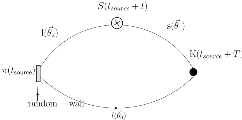
Figure 1: Structure of the 3-point functions needed to calculate $f_{0}^{K\pi}(q^{2})$. Light-quark propagators are generated at $t_{source}$ with random-wall sources. An extended strange propagator is generated at $T$.

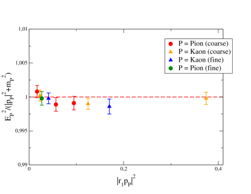
Figure 2: Deviation of our data from the continuum dispersion relation prediction.

We found in a previous test run [7] that the use of random-wall sources greatly reduces the statistical errors of the parameters of the two-point and three-point correlators, so we use them throughout this analysis.

3 Simulation details and fitting

We have completed the generation of correlators with HISQ staggered valence quarks on the $2+1$ flavor asqtad staggered MILC ensembles [8] shown in Table 1 at two lattice spacings.

	$\approx a$ (fm)	$am_{l}/am_{h}$	$N_{conf}$	$am_{s}^{val}$	$am_{l}^{val}$	$N_{sources}$	$N_{T}$
coarse	$0.12$	$0.020/0.050$	$2052$	$0.0491(9)$	$0.02806$	$4$	$5$
		$0.010/0.050$	$2243$	$0.0495(9)$	$0.01414$	$4$	$8$
		$0.005/0.050$	$2098$	$0.0489(9)$	$0.00670$	$8$	$5$
fine	$0.09$	$0.0124/0.031$	$1996$	$0.0337(6)$	$0.0080$	$4$	$5$
		$0.0062/0.031$	$1946$	$0.0336(6)$	$0.0160$	$4$	$5$

Table 1: Ensembles and simulation details. $am_{h}$ is the nominal strange-quark mass in the sea sector, $N_{sources}$ is the number of time sources, and $N_{T}$ the number of sink-source separations for which we have generated data.

We average results over four time sources separated by 16 (24) timeslices on the $0.12~{}{\rm fm}$ ($0.09~{}{\rm fm}$) ensembles but displaced by a random distance from configuration to configuration to suppress autocorrelations. A subset of this data was analyzed in [7]. The strange valence mass is tuned to its physical value on each ensemble [4]. The valence light-quark masses are fixed according to the relation, $\frac{m_{l}^{val}(HISQ)}{m_{s}^{phys.}(HISQ)}=\frac{m_{l}^{sea}(asqtad)}{m_{s}^{phys.}(asqtad)}$. The effect of the mixed actions for the sea and valence quark sectors can be analyzed using partially quenched staggered CHPT techniques for the chiral and continuum extrapolations.

We fit the two-point functions for a pseudoscalar meson $P$ to the expression

$$C_{2pt}^{P}(\vec{p}_{P};t) = \sum_{m=0}^{N_{exp}}(-1)^{mt}(Z_{m}^{P})^{2}\left(e^{-E_{P}^{m}t}+e^{-E_{P}^{m}(L_{t}-t)}\right)\,,$$ (5)

where $L_{t}$ is the temporal size of the lattice. Oscillating terms with $(-1)^{m}$ do not appear for pions with zero momentum. From two-point function fits, we checked whether the continuum dispersion relation is satisfied. This is plotted in Fig. 2, which shows very small deviations from the continuum prediction ($\leq 0.15\%$), indicating small discretization effects.

The functional form for the three-point functions is

$$C_{3pt}^{K\to\pi}(\vec{p}_{\pi},\vec{p}_{K};t,T) = \sum_{m,n=0}^{N_{exp}^{3pt}}(-1)^{mt}(-1)^{n(T-t)}A^{mn}Z_{m}^{\pi}Z_{n}^{K}\left(e^{-E_{\pi}^{m}t-E_{\pi}^{m}(L_{t}-t)}\right)\left(e^{-E_{K}^{n}(T-t)-E_{K}^{n}(T-L_{t}+t)}\right)\,,$$

where the factors $Z_{i}^{P}$ are the amplitudes of the two-point functions in (5). The three-point parameter $A^{00}$ in (3) is related to the desired form factor $f_{0}^{K\pi}(q^{2})$ via $f_{0}^{K\pi}(q^{2})=\frac{1}{2}A^{00}(q^{2})\,\sqrt{2E_{\pi}E_{K}}\,(m_{s}-m_{l})/(m_{K}^{2}-m_{\pi}^{2})$, where we have used (3) and taken into account some overall factors involved in the parametrization of the correlation function. We extract the form factors $f_{0}^{K\pi}(q^{2})$ using the expression above directly from simultaneous fits of the relevant three- and two-point functions. In these fits we include several three-point functions with different values of the source-sink separation $T$, with at least one odd $T$ and one even $T$ to be able to get a handle on the contributions from the oscillatory states.

In this analysis it is especially relevant to check for the stability of our fits under the choice of fitting parameters and techniques, since we are getting very small statistical errors and we need to be sure that these results are not methodology dependent in any way. One of the checks we performed is varying the time fitting ranges and number of states included in the fits. Fitting ranges for two-point functions are $t_{min}-(L_{t}-t_{min})$ and for the three-point functions $t_{min}-(T-t_{min})$, with $L_{t}$ the temporal size of the lattice and $T$ the source-sink separation—see Fig. 2. The number of states included is the same in the regular and oscillating sectors, so $N_{exp}=N_{{\rm regular\,states}}=N_{{\rm oscillatory\,states}}$. Fixing $N_{exp}$ and changing $t_{min}$ from 3 (5) for $0.12~{}{\rm fm}$ ($0.09~{}{\rm fm}$) ensembles up to the maximum allowed by the source-sink separation, give us a plateau for central values with only small variations in errors. Analogously, fixing $t_{min}$ to our preferred value we do not find any significant variation of results for $N_{exp}\geq 3-4$.

We study as well which combination of $T^{\prime}s$ from the ones we have simulated is optimal. We find that the central values are very insensitive to the number of three-point functions included and the values of $T$ in the range we are analyzing. Errors and stability are better when $15\leq T\leq 24$ and including three three-point functions for the $0.12~{}{\rm fm}$ ensembles, and $18\leq T\leq 33$ and including four three-point functions for the $0.09~{}{\rm fm}$ ensembles.

Finally, we checked an alternative way of doing the fits, using the iterative superaverage method described in [9]. This takes an explicit combination of three-point functions with consecutive values of $T$ and the time slice $t$ which suppresses the contribution from both the first regular excited state and the first oscillatory state. Again, results are compatible within one statistical $\sigma$ with our preferred fitting method.

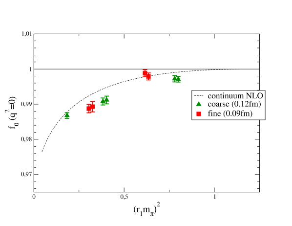
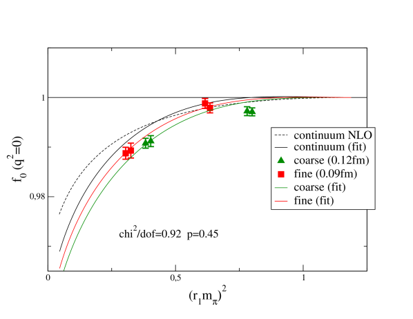
Figure 3: In the left panel, we collect the form factor $f_{+}^{K\pi}(0)$ obtained from the different ensembles in Table [1]. The right panel shows an example of the output from the chiral and continuum extrapolation tests. The dotted black line in both plots is the NLO CHPT prediction. The solid black line is the extrapolation in the light-quark mass with a physical $m_{s}$ and in the continuum limit. The green and red lines are also extrapolations in the light-quark masses with $m_{s}^{phys}$ but with $a\approx 0.12~{}{\rm fm},0.09~{}{\rm fm}$, respectively.

4 Results for $f_{+}(q^{2}=0)$

In Fig. 3 we collect the results for $f_{+}^{K\pi}(0)$ with statistical errors from our preferred fits as a function of $(r_{1}m_{\pi})^{2}$, fixing $(2m_{K}^{2}-m_{\pi}^{2})$ to the experimental value. We plot results coming from three-point functions where the external momentum to obtain $q^{2}=0$ is injected via the $K$ and the $\pi$ (we give an offset in the pion mass to the two points for clarity). The green triangle at the far left corresponds to the $0.12~{}{\rm fm}$ ensemble with masses 0.005/0.050, four time sources, and a moving pion. When analyzing those data we found it to be more challenging to get stable results, so we have decided to double the number of sources and exclude it in our discussions until the full new data set is analyzed and other effects, like finite volume corrections, are incorporated to the analysis. So, in particular, we do not include it in the fits described below.

The first remarkable characteristic of our results is that the statistical errors are very small, $0.1-0.15\%$, reaching our goal to be competitive with other determinations. In addition, the results coming from three-point functions where the external momentum to get $q^{2}=0$ is injected via the $K$ and the $\pi$ agree within the very small statistical errors, as can be seen in the figure. This constitutes a very good test of our methodology and quoted errors.

4.1 Chiral and continuum extrapolation

The form factor $f_{+}(0)$ can be written as a CHPT expansion in the following way: $f_{+}(0)=1+f_{2}+f_{4}+f_{6}+...=1+f_{2}+\Delta f$. The Ademollo-Gatto (AG) theorem, which follows from vector current conservation, ensures that $f_{+}(0)\to 1$ in the $SU(3)$ limit and, furthermore, that the $SU(3)$ breaking effects are second order in $(m_{K}^{2}-m_{\pi}^{2})$. This fixes $f_{2}$ completely in terms of experimental quantities. At finite lattice spacing, systematic errors can enter due to, for example, corrections to the dispersion relation needed to derive Eq. (3). Those and other discretization effects are very small though, as can be deduced from our results in Fig. 3. However, since statistical errors are at the $0.1-0.2\%$ level, we should pin down the other sources of systematic errors as precisely as possible.

Our plan for treating the light-quark mass dependence and the discretization effects in our calculation is to use two-loop continuum CHPT [10], supplemented by staggered partially quenched CHPT at one-loop. The small variation with $a$ in our data suggests that addressing those effects at one loop should be enough for our target precision.

Since we do not yet have the staggered CHPT expressions, nor have we implemented the two-loop continuum CHPT functions, just as an exercise, we can try to fit our data with a much more simple fitting ansatz. We take the continuum partially quenched NLO CHPT expression [11] and add a general parametrization of NNLO analytic terms and $a^{2}$ corrections of the form

$$f_{+}^{K\pi}(0)=1+f_{2}+C_{a}\left(\frac{a}{r_{1}}\right)^{2}+ r_{1}^{4}(m_{\pi}^{2}-m_{K}^{2})^{2}\Big{[}C_{6}^{(1)}(r_{1}m_{\pi})^{2}+C_{6}^{(2)}(r_{1}m_{K})^{2}$$

$$+ C_{6}^{(3)}(r_{1}m_{\pi})^{2}log(m_{\pi}^{2}/\mu^{2})+C_{6}^{(4)}(r_{1}m_{\pi})^{4}+C_{6}^{(5)}\left(\frac{a}{r_{1}}\right)^{2}\Big{]}.$$ (7)

We include only correlation functions coming from injecting the momentum in the $\pi$ for these test fits. The result for one of these fits with $C_{a}=C_{6}^{(i)}=0$ for $i=3,4$ is shown in Fig. 3. We can obtain similar good fits with different combinations of terms in (4.1). This must be taken just as a naive first try to fit our data and no conclusions should be drawn until we have used staggered CHPT to gain more information about the $a^{2}$ structure of our data.

5 Conclusions and outlook

We have completed the generation of the data in Table 1 needed for the calculation of $f_{+}^{K\pi}(0)$. Since the time of the conference we have generated data for another coarse ensemble with light-quark mass $am_{l}=0.007$ to facilitate the chiral extrapolation, which we anticipate is going to be our main source of uncertainty.

The statistical errors in the form factor in all ensembles exceed our expectations, being around $0.1-0.15\%$. We have performed several checks of the robustness of the central fit values and errors, by studying the stability with changes in the time range and number of states, the dependence on the source-sink separation and number of three-point functions included in the fit, and testing alternative methods for fitting the correlation functions. We find it very difficult to make changes in the fitting procedure that change the fit results outside the one sigma range. Another very good test of our results is the fact that $f_{+}^{K\pi}(0)$ as extracted from three-point correlation functions with a moving $\pi$ and a moving $K$ agree with each other. For the final analysis we will redo the fits we found to be the optimal, including the correlation functions with both momentum injected in the $\pi$ and the $K$ to further increase the statistics.

We found very small lattice spacing dependence in our data and the continuum dispersion relation is fulfilled at the $0.15\%$ level, but in view of the small statistical error, we plan to study in detail the dependence on $a^{2}$ by using staggered partially quenched CHPT at one-loop. We will also investigate the use of two-loop continuum CHPT.

With all these elements, we expect our calculation to be competitive with the current state of the art.

- [1] M. Antonelli et al., Eur. Phys. J. C69, 399-424 (2010). [arXiv:1005.2323 [hep-ph]].
- [2] H. Na, C. T. H. Davies, E. Follana, G. P. Lepage, J. Shigemitsu, Phys. Rev. D82 (2010) 114506. [arXiv:1008.4562 [hep-lat]].
- [3] V. Lubicz et al. [ETM Collaboration], Phys. Rev. D80 (2009) 111502. [arXiv:0906.4728 [hep-lat]]; P. A. Boyle et al., Eur. Phys. J. C69 (2010) 159-167. [arXiv:1004.0886 [hep-lat]].
- [4] C. T. H. Davies, E. Follana, I. D. Kendall, G. P. Lepage and C. McNeile [HPQCD Collaboration], Phys. Rev. D 81 (2010) 034506 [arXiv:0910.1229 [hep-lat]].
- [5] P. F. Bedaque, J. -W. Chen, Phys. Lett. B616, 208-214 (2005). [hep-lat/0412023].
- [6] P. A. Boyle et al. [RBC-UKQCD Collaboration], Eur. Phys. J. C69 (2010) 159-167. [arXiv:1004.0886 [hep-lat]].
- [7] J. A. Bailey et al. [Fermilab Lattice and MILC Collaboration], PoS LATTICE2010 (2010) 306. [arXiv:1011.2423 [hep-lat]].
- [8] A. Bazavov et al., Rev. Mod. Phys. 82 (2010) 1349-1417. [arXiv:0903.3598 [hep-lat]].
- [9] J. A. Bailey et al., Phys. Rev. D79 (2009) 054507. [arXiv:0811.3640 [hep-lat]].
- [10] J. Bijnens, P. Talavera, Nucl. Phys. B669 (2003) 341-362. [hep-ph/0303103].
- [11] Johan Bijnens, private communication.