The Loschmidt Echo as a robust decoherence quantifier for many-body systems

Abstract

We employ the Loschmidt Echo, i.e. the signal recovered after the reversal of an evolution, to identify and quantify the processes contributing to decoherence. This procedure, which has been extensively used in single particle physics, is here employed in a spin ladder. The isolated chains have $1/2$ spins with $XY$ interaction and their excitations would sustain a one-body like propagation. One of them constitutes the controlled system $\mathcal{S}$ whose reversible dynamics is degraded by the weak coupling with the uncontrolled second chain, i.e. the environment $\mathcal{E}$. The perturbative $\mathcal{SE}$ coupling is swept through arbitrary combinations of $XY$ and Ising like interactions, that contain the standard Heisenberg and dipolar ones. Different time regimes are identified for the Loschmidt Echo dynamics in this perturbative configuration. In particular, the exponential decay scales as a Fermi golden rule, where the contributions of the different $\mathcal{SE}$ terms are individually evaluated and analyzed.  Comparisons with previous analytical and numerical evaluations of decoherence based on the attenuation of specific interferences, show that the Loschmidt Echo is an advantageous decoherence quantifier at any time, regardless of the $\mathcal{S}$ internal dynamics.

I INTRODUCTION

The physical realization of Quantum Information Processing (QIP) Bennett and DiVincenzo (2000), requires a precise control of quantum dynamics. The coherent manipulation of many-body systems plays a crucial role for several QIP-related implementations, such as spintronic devices Awschalom and Flatté (2007), optical lattices Bloch et al. (2008); Sherson et al. (2010), superconducting circuits Dicarlo et al. (2010) and nitrogen-vacancy centers in diamond Grinolds et al. (2011). Experiments with spin arrays in Nuclear Magnetic Resonance (NMR) Levstein et al. (1998); Pastawski et al. (2000); Krojanski and Suter (2004), have shown that many-body dynamics conspires against quantum control. Moreover, once the system interacts with an environment, control becomes even more difficult due to information leakage. This degradation of the system’s coherent dynamics, called decoherence, is subject of deep theoretical and experimental investigation Zurek et al. (2007), as it remains the key obstacle for QIP. Indeed, quantum error correction protocols Kosut et al. (2008); Knill and Laflamme (1997) can restore quantum information provided that they operate above a certain threshold. Achieving this limit is often a task for dynamical decoupling techniques Viola et al. (1999); Ryan et al. (2010); Álvarez et al. (2010a). However, specific implementations require a precise knowledge of the nature of the decoherence processes Ladd et al. (2010). It is the purpose of this paper to contribute to a better characterization of the role of a spin environment on the decoherence of a many-spin system.

At least for short distance communications, spin chains can be used to transfer information Bose (2003). In fact, several selective polarization techniques have been developed in NMR experiments to set up an initial local excitation in one edge of a spin chain and transfer it to the other edge by means of an effective $XY$ Hamiltonian (i.e. $S_{i}^{+}S_{j}^{-}+S_{i}^{-}S_{j}^{+}$ or polarization conserving ”flip-flop” processes) Mádi et al. (1997); Cappellaro et al. (2007). Additionally, Multiple Quantum Coherence spectroscopy has allowed the study of quasi-one-dimensional spin systems under the influence of spin environments Zhang et al. (2009); Rufeil-Fiori et al. (2009). Here, the Double Quantum Hamiltonian (i.e. the $S_{i}^{+}S_{j}^{+}+S_{i}^{-}S_{j}^{-}$ processes), can be mapped to an $XY$ Hamiltonian allowing the design and control of the excitation transfer in a broader family of solid-state spin structures Fel’dman and Lacelle (1997); Doronin et al. (2000); Doronin and Fel’dman (2005); Cappellaro et al. (2007); Ramanathan et al. (2011). Thus, a deep knowledge of decoherence in such 1-D systems is crucial to improve the degree of control available for NMR-based state transfer protocols Álvarez et al. (2010b); Cappellaro et al. (2011).

A natural way to quantify the decoherence time $\tau_{\phi}$ is through the degradation of interferences. This requires the identification of specific coherence “witnesses”, such as excitations in the local polarization. Particularly useful are the reflections in the boundaries that can be observed as well defined Mesoscopic Echoes (ME) Pastawski et al. (1995); Pastawski (1996); Prigodin et al. (1994). Recently, the ME intensity has been used to quantify decoherence of spins arranged in a ladder topology Álvarez et al. (2010c). Alternatively, the evaluation of $\tau_{\phi}$ can be performed by a time reversal procedure, the Loschmidt Echo (LE) Jalabert and Pastawski (2001), where one evaluates the reversibility of the system’s dynamics in the presence of an uncontrolled environment. The LE can be accessed experimentally in many situations, such as spin systems Pastawski et al. (2000); Levstein et al. (1998); Sánchez et al. (2009), confined atoms Andersen et al. (2006) and microwave excitations Schäfer et al. (2005). Besides, it has become a standard way to quantify decoherence, stability and complexity in dynamical processes, in several physical situations Jacquod and Petitjean (2009); Gorin et al. (2006); *loschScholarpedia.

In the present article, we address the controllability of a spin chain ($\mathcal{S}$) in the presence of a spin environment ($\mathcal{E}$) by performing a quantitative study of the LE. The LE degradation characterizes the decoherence due to the perturbation of $\mathcal{E}$ on the otherwise simple dynamics of $\mathcal{S}$. Indeed, the many-body nature of the $\mathcal{S}$-$\mathcal{E}$ interaction yields a very rich behavior in the dynamical regimes of decoherence: a short time quadratic decay, an exponential regime, and a saturation plateau are identified by our numerical approach. In particular, we perform a detailed analysis of the LE exponential decay, addressing how the rates scale with a Fermi golden rule (FGR). Additionally, since for weak perturbations the LE of the local excitation can be seen as a Survival Probability (SP), the numerical results are compared to previous analytical predictions for that magnitude Flambaum and Izrailev (2001).

In the next section, we describe the spin problem and summarize its theoretical background. We introduce the spin autocorrelation function and describe a single particle analogy which underlies further analysis. We also discuss the local version of the Loschmidt Echo and present its definition in terms of the local polarization, which is the usual experimental observable. In Section III.1, we present the numerical study of the LE for some of the different physically relevant parameters. We consider $\mathcal{S}$-$\mathcal{E}$ interactions which are weak compared with those determining the $\mathcal{E}$ dynamics. We also address different anisotropies of the $\mathcal{S}$-$\mathcal{E}$ interaction which ranges from pure $XY$ (planar) to truncated dipolar cases, going through the Heisenberg (isotropic) interaction. In Section III.2 we analyze the obtained results. First we consider the transition from the short time quadratic decay to the exponential regime in analogy to what is known for the SP. Then, we focus on the exponential regime to show that the Fermi golden rule in the present spin problem has independent contributions arising from each specific process in the $\mathcal{S}$-$\mathcal{E}$ interaction. We then compare these rates with a previous evaluation based on the contrast of specific interferences (ME attenuation). In the last section, we conclude that since the LE filters the internal dynamics of the system, it provides a reliable and continuous access to all time regimes. Thus, the LE compares favorably with the evaluation of decoherence based on interference contrast.

II QUANTUM DYNAMICS IN SPIN SYSTEMS

II.1 THE MODELS

The spin models analyzed in this article are schematized in Fig. 1. In the first one, the system $\mathcal{S}$ is an $m$-spin chain (Fig. 1-a), which could constitute a quantum channel. It interacts with a second chain $\mathcal{E}$, that stands for the “environment” which perturbs the dynamics of $\mathcal{S}$. The second model (Fig. 1-b) is obtained from the first one by imposing a periodic boundary condition that transforms chains into rings.

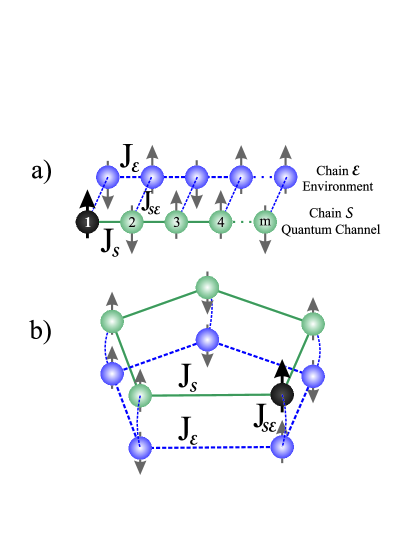
Figure 1: (Color Online). The spin system. (a) Open boundary conditions. (b) Closed boundary conditions (ring-like). Continuous (green) connections represent interactions that can be inverted to obtain the Loschmidt echo. Dash (blue) lines represent non-controllable interactions. The first spin (black circle) is initially polarized and the rest of the spins are in one of the high temperature configurations.

For both models, the spin Hamiltonian is given by:

$$\hat{H}_{total}=\hat{H}_{\mathcal{S}}\otimes\hat{I}_{\mathcal{E}}+\hat{I}_{\mathcal{S}}\otimes\hat{H}_{\mathcal{E}}+\hat{V}_{\mathcal{SE}},$$ (1)

where the first and second terms represent the system and the environment Hamiltonians respectively, and the third one is the interaction between them. In order to simplify notation, we write just $\hat{H}_{\mathcal{S}}$ and $\hat{H}_{\mathcal{E}}$ instead of the tensor product with their respective $\hat{I}_{\mathcal{E}}$ and $\hat{I}_{\mathcal{S}}$ identities. For both $\mathcal{\nu}=\mathcal{S}$ or $\mathcal{E}$, we use an effective “planar” or $XY$ Hamiltonian Mádi et al. (1997), that describes the homogeneous flip-flop interaction between nearest neighbor spins. In the model of Fig. 1-a, i.e. the chain:

$$\hat{H}_{\nu} =\sum_{n=1}^{m-1}J_{\nu}(\hat{S}_{\mathcal{\nu},n+1}^{x}\hat{S}_{\mathcal{\nu},n}^{x}+\hat{S}_{\mathcal{\nu},n+1}^{y}\hat{S}_{\mathcal{\nu},n}^{y})$$

$$=\sum_{n=1}^{m-1}\frac{J_{\nu}}{2}(\hat{S}_{\mathcal{\nu},n+1}^{+}\hat{S}_{\mathcal{\nu},n}^{-}+\hat{S}_{\mathcal{\nu},n+1}^{-}\hat{S}_{\mathcal{\nu},n}^{+}).$$ (2)

Here $\hat{S}_{\mathcal{\nu},n}^{x}$ and $\hat{S}_{\mathcal{\nu},n}^{y}$ are the $x$ and $y$ components of the spin operator in the $n$-th site in the $\nu$ chain respectively, while $\hat{S}_{\mathcal{\nu},n}^{+}$ and $\hat{S}_{\mathcal{\nu},n}^{-}$ are the raising and lowering operators. Again, the abbreviated notation for any spin operator must be understood in the form $\hat{S}_{\mathcal{S},n}^{z}=\hat{I}_{1}\otimes\ldots\otimes\hat{S}_{n}^{z}\otimes\ldots\otimes\hat{I}_{m}\otimes\hat{I}_{m+1}\otimes\ldots\otimes\hat{I}_{2m}$. If one wants to consider the ring model, an extra $XY$ coupling appears between the $1$-st and $m$-th spins.

The interchain coupling is:

$$\hat{V}_{\mathcal{SE}} =\sum_{n=1}^{m}J_{\mathcal{SE}}[2\alpha\hat{S}_{\mathcal{S},n}^{z}\hat{S}_{\mathcal{E},n}^{z}-(\hat{S}_{\mathcal{S},n}^{x}\hat{S}_{\mathcal{E},n}^{x}+\hat{S}_{\mathcal{S},n}^{y}\hat{S}_{\mathcal{E},n}^{y})]$$ (3)

$$=\sum_{n=1}^{m}J_{\mathcal{SE}}[2\alpha\hat{S}_{\mathcal{S},n}^{z}\hat{S}_{\mathcal{E},n}^{z}-\frac{1}{2}(\hat{S}_{\mathcal{S},n}^{+}\hat{S}_{\mathcal{E},n}^{-}+\hat{S}_{\mathcal{S},n}^{-}\hat{S}_{\mathcal{E},n}^{+})],$$ (4)

where the first term is an Ising interaction. The $\alpha$ parameter determines the anisotropy of the coupling. This encompass the typical magnetic resonance scenarios: the $XY$ (planar) interaction Mádi et al. (1997), represented by $\alpha=0$; the Heisenberg (isotropic) interaction Levstein et al. (1991), by $\alpha=-\frac{1}{2}$; and the truncated dipolar coupling Zhang et al. (1992) corresponds to $\alpha=1$. In order to extend and systematize our analysis we also consider several other values for $\alpha$. It is important to notice that for any finite $\alpha$ the $\mathcal{S}$-$\mathcal{E}$ interaction has always an $XY$ component. This allows a polarization exchange which, in a Fermionic representation, can be seen as a “single-particle tunnelling” Danieli et al. (2004). In such a picture, the Ising term corresponds to a nearest neighbour Hubbard term which is a two-body interaction.

It is crucial to stress that the real constants $J_{\mathcal{S}}$, $J_{\mathcal{E}}$ and $J_{\mathcal{SE}}$ determine the relevant time scales of the whole dynamics. As introduced above, the first two give the homogeneous $XY$ coupling within $\mathcal{S}$ and $\mathcal{E}$ respectively, while $J_{\mathcal{SE}}$ stands for the interchain coupling. To ensure a smooth degradation of the $\mathcal{S}$ coherent dynamics, we set $J_{\mathcal{SE}}$ in the weak coupling limit, i.e. $J_{\mathcal{SE}}\ll$ $J_{\mathcal{S}}=J_{\mathcal{E}}$.

II.2 Basic features of Spin Dynamics

A natural question for the spin models introduced above is how to quantify the decoherence of $\mathcal{S}$ in the presence of $\mathcal{E}$. This means that one has to deal with a composite (bipartite) Hilbert space $\mathcal{S\otimes E}$, and trace out the $\mathcal{E}$-degrees of freedom whenever necessary. A standard strategy relies on finding an appropriate decoherence rate $1/\tau_{\phi}$ through the quantification of the attenuation of system’s specific interferences. As in the experiments Zhang et al. (1992); Pastawski (1996), one starts evaluating the evolution of an injected local polarization through the spin autocorrelation function Abragam (1986); Levstein et al. (1991):

$$P_{1,1}(t)=\frac{\left\langle\Psi_{eq}\right|\hat{S}_{\mathcal{S},1}^{z}(t)\hat{S}_{\mathcal{S},1}^{z}(0)\left|\Psi_{eq}\right\rangle}{\left\langle\Psi_{eq}\right|\hat{S}_{\mathcal{S},1}^{z}(0)\hat{S}_{\mathcal{S},1}^{z}(0)\left|\Psi_{eq}\right\rangle}.$$ (5)

This function gives the local polarization at time $t$ along the $z$ direction in site $1$ provided that at time $t=0$ the system was in its thermal equilibrium state plus a local excitation in site $1$. Here, the spin operator in the Heisenberg representation is given by $\hat{S}_{\mathcal{S},1}^{z}(t)=e^{\mathrm{i}\hat{H}_{total}t/\hbar}\hat{S}_{\mathcal{S},1}^{z}e^{-\mathrm{i}\hat{H}_{total}t/\hbar}$. The many-body state $\left|\Psi_{eq}\right\rangle$ corresponding to a high temperature thermal equilibrium represents a mixture of all states with amplitudes satisfying the appropriate statistical weights and random phases. Then, the initial non-equilibrium local excitation $\left|\Psi_{ne}\right\rangle$ can be defined in terms of the computational (Ising) basis components that have the $1^{\mathrm{st}}$ spin up as:

$$\left|\Psi_{ne}\right\rangle=\frac{\hat{S}_{\mathcal{S},1}^{+}\left|\Psi_{eq}\right\rangle}{\left|\left\langle\Psi_{eq}\right|\hat{S}_{\mathcal{S},1}^{-}\hat{S}_{\mathcal{S},1}^{+}\left|\Psi_{eq}\right\rangle\right|^{1/2}}=\sum_{r}c_{r}\left|\Psi_{r}\right\rangle,$$ (6)

see Appendix A for further details. Here, each contribution $\left|\Psi_{r}\right\rangle$ to the locally polarized initial state can be written as:

$$\left|\Psi_{r}\right\rangle=\left|\uparrow_{1}\right\rangle\otimes\left|\beta_{r}\right\rangle,$$ (7)

where the basis for the remaining $2m-1$ spins is

$$\left|\beta_{r}\right\rangle=\left|s_{2}\right\rangle\otimes\left|s_{3}\right\rangle\otimes\left|s_{4}\right\rangle\otimes...\otimes\left|s_{2m}\right\rangle\ \text{\ with }\left|s_{k}\right\rangle\in\left\{\left|\uparrow\right\rangle,\left|\downarrow\right\rangle\right\}.$$ (8)

Since in the regime of NMR spin dynamics, the thermal energy $k_{B}T$ is much higher than any other energy scale of the system Slichter (1980); Abragam (1986), all statistical weights result identical, i.e. $\left|c_{r}\right|=1/\sqrt{2^{2m-1}}.$

It is useful to analyze the autocorrelation $P_{1,1}(t)$. For each contribution $\left|\Psi_{r}\right\rangle$ to the initial state, the evolved wave function at time $t$, is

$$\left|\Psi_{r}(t)\right\rangle=\exp\{-\tfrac{\mathrm{i}}{\hbar}\hat{H}_{total}t\}\left|\Psi_{r}\right\rangle.$$ (9)

Then, the probability of finding the first spin up-polarized is:

$$P_{1,1}^{\left[r\right]}(t)=\sum_{j}\left|(\left\langle\uparrow_{1}\right|\otimes\left\langle\beta_{j}\right|)\left|\Psi_{r}(t)\right\rangle\right|^{2},$$ (10)

where the sum runs over the 2^2m-1 configurations of the $2m-1$ remaining spins. Notice that the sum over the $j$-index in Eq. 10, means that we are performing a trace not only over $\mathcal{E}$, but also over the spins in $\mathcal{S}$ other than the first one. After the summation over all contributions $\left|\Psi_{r}\right\rangle$ to the initial state, and expressing the result as a local polarization Pastawski et al. (1995), we obtain:

$$P_{1,1}(t)=\bigg{[}\sum_{r=1}^{2^{2m-1}}\left|c_{r}\right|^{2}P_{1,1}^{\left[r\right]}(t)-\frac{1}{2}\bigg{]}\times 2.$$ (11)

A computation of the time dependent local observable in Eq. 5 reduces to Eq. 11 which in turn, requires evolving each of the $2^{2m-1}$ pure states to evaluate the ensemble averaged observables. This is implemented using a Trotter decomposition Rieth and Schommers (2006) assisted by an algorithm that exploits quantum parallelism Álvarez et al. (2008) (See appendix B).

II.3 The single-particle picture and Mesoscopic Echoes

The obvious complexity of the many spin dynamics might hinder some simple interference phenomena that can be taken as hallmarks. Under certain experimentally achievable conditions (e.g. $XY$ interaction, 1D topology and negligible $\mathcal{S}$-$\mathcal{E}$ interaction), the autocorrelation $P_{1,1}(t)$ becomes a simple one-body magnitude. Indeed, once the initial excitation is created, the first physical picture about its evolution may be obtained from the Wigner-Jordan spin-fermion mapping Lieb et al. (1961). The point here is to trace over the $\mathcal{E}$-degrees of freedom from the beginning and focus on a single quantum spin chain. Accordingly, an isolated $m$ spin chain with $XY$ interaction, where $N$ of them are up, is mapped to a chain with $N$ non-interacting fermions. Thus, a local polarization excitation has the same dynamics as a single fermion wave-packet in a tight-binding linear chain Danieli et al. (2004, 2005). The observed autocorrelation function in the limit of infinite temperature is precisely described by the evolution of a single spin up in a chain of down spins:

$$\left|\Psi_{1}\right\rangle:=\left|\uparrow_{1}\right\rangle\otimes\left|\downarrow_{2}\right\rangle\otimes\left|\downarrow_{3}\right\rangle\otimes...\otimes\left|\downarrow_{m}\right\rangle.$$ (12)

This is a one-body wave function, defined on a subspace of $\mathcal{S}$ where the total spin projection is $\frac{m}{2}-1$, and the observable is evaluated as:

$$P_{1,1}^{\left[r=1\right]}(t)=\left|\left\langle\Psi_{1}\right|\exp[-\mathrm{i}\hat{H}_{\mathcal{S}}t/\hbar]\left|\Psi_{1}\right\rangle\right|^{2}.$$ (13)

Since this is a finite size system one should expect revivals of the initial polarization. Such revivals are called Mesoscopic Echoes (ME) Prigodin et al. (1994); Pastawski et al. (1995) and they appear when constructive interferences manifest at the Heisenberg time $t_{H}\sim\hbar/\Delta$, with $\Delta$ being the typical mean energy level spacing. In a spin chain with $XY$ interaction one may safely use $\Delta\simeq J_{\mathcal{E}}/m$. As long as such one-body picture remains approximately valid for a linear chain weakly coupled to the environment these interferences show up experimentally Pastawski (1996); Mádi et al. (1997); Khitrin and Fung (1999).

A weak coupling to the spin bath $\mathcal{E}$ results in a progressive attenuation of the ME, which has been used to quantify environmentally induced decoherence Álvarez et al. (2010c). This attenuation is understood as a Fermi golden rule (FGR), which describes an “irreversible” decay of a pure state in $\mathcal{S}$ into collective $\mathcal{S\otimes E}$ states. In fact, the validity of the FGR requires here the breakdown of degeneracies, i.e. the whole $\mathcal{S}\otimes\mathcal{E}$ must behave as a fully many-body system. We shall return to this point below.

II.4 Loschmidt Echo

Let us now explain the essence of the protocol that uses the Loschmidt Echo to quantify decoherence in a spin system using a local spin as an observable Levstein et al. (1998). Our strategy relies on the controllability of the chain $\mathcal{S}$, whose Hamiltonian’s sign can be switched at will as it is often the case in NMR. The reversibility of the dynamics within the chain is perturbed by the interaction with the non-controlled spin chain $\mathcal{E}$. There are two stages in the evolution. First, a spin excitation is created and the whole spin set evolves according to the Hamiltonian of Eq. 1, during a time $t_{R}$. At that time, the internal interactions within $\mathcal{S}$ are reversed (i.e. $\hat{H}_{\mathcal{S}}$ is replaced by $-\hat{H}_{\mathcal{S}}$ during a second $t_{R}$-period). However, neither the $\mathcal{S}$-$\mathcal{E}$ coupling nor the interactions within chain $\mathcal{E}$ are reversed, leading to a non-reversed perturbation,

$$\hat{\Sigma}=\hat{H}_{\mathcal{E}}+\hat{V}_{\mathcal{SE}},$$ (14)

acting in both periods. Thus, in analogy with Eq. 5, we define the observable Loschmidt echo as the recovered local polarization:

$$M_{LE}(2t_{R})=\frac{\left\langle\Psi_{eq}\right|\hat{S}_{\mathcal{S},1}^{z}(2t_{R})\hat{S}_{\mathcal{S},1}^{z}(0)\left|\Psi_{eq}\right\rangle}{\left\langle\Psi_{eq}\right|\hat{S}_{\mathcal{S},1}^{z}(0)\hat{S}_{\mathcal{S},1}^{z}(0)\left|\Psi_{eq}\right\rangle}.$$ (15)

The spin operators, expressed in the Heisenberg representation, are now:

$$\hat{S}_{\mathcal{\nu},1}^{z}(2t_{R})=e^{\frac{\mathrm{i}}{\hbar}(-\hat{H}_{\mathcal{S}}+\hat{\Sigma})t_{R}}e^{\frac{\mathrm{i}}{\hbar}(\hat{H}_{\mathcal{S}}+\hat{\Sigma})t_{R}}\hat{S}_{\mathcal{\nu},1}^{z}e^{-\frac{\mathrm{i}}{\hbar}(\hat{H}_{\mathcal{S}}+\hat{\Sigma})t_{R}}e^{-\frac{\mathrm{i}}{\hbar}(-\hat{H}_{\mathcal{S}}+\hat{\Sigma})t_{R}}.$$ (16)

The computation of the Loschmidt Echo in Eq. 15 proceeds as we did above for the forward dynamics. In a system with a general interaction, it requires a full many-body evolution.

As before, the initial excitation is described in terms of the Ising basis by Eq. 6. For each contribution $\left|\Psi_{r}\right\rangle$ to the initial state, the resulting wave function at time $t=2t_{R}$, after the whole time-reversal procedure, is

$$\left|\Psi_{r}(2t_{R})\right\rangle=\exp\{-\tfrac{\mathrm{i}}{\hbar}(-\hat{H}_{\mathcal{S}}+\hat{\Sigma})t_{R}\}\exp\{-\tfrac{\mathrm{i}}{\hbar}(\hat{H}_{\mathcal{S}}+\hat{\Sigma})t_{R}\}\left|\Psi_{r}\right\rangle.$$ (17)

In analogy with the discussion above, the probability of finding the first spin up-polarized is:

$$M_{1,1}^{\left[r\right]}(t)=\sum_{j}\left|(\left\langle\uparrow_{1}\right|\otimes\left\langle\beta_{j}\right|)\left|\Psi_{r}(t)\right\rangle\right|^{2},$$ (18)

where the sum runs over the 2^2m-1 configurations of the $2m-1$ remaining spins. Again, the sum over $j$ means a trace over all the spins of the environment and the system except the first one. After the summation (average) over all contributions $\left|\Psi_{r}\right\rangle$ to the initial state, and expressing the result as a local polarization, we compute the local Loschmidt Echo as:

$$M_{LE}(t)=\bigg{[}\sum_{r=1}^{2^{2m-1}}\left|c_{r}\right|^{2}M_{1,1}^{\left[r\right]}(t)-\frac{1}{2}\bigg{]}\times 2.$$ (19)

Here again, the statistical weights $\left|c_{r}\right|^{2}$ are the inverse of $2^{2m-1},$ the number of initial states  in the ensemble that satisfy the “$1^{\mathrm{st}}$ spin up polarized” condition. Notice that, except for the fact that the evolution operator contains a partially reversed dynamics, this quantity refers to the same physical observable as Eq. 11.

II.5 Connection to previous works

It would be useful to make a connection between the observable just described and the usual definition of the Loschmidt Echo Jalabert and Pastawski (2001), which was extensively studied in the field of quantum chaos and quantum information Jacquod and Petitjean (2009); Gorin et al. (2006); *loschScholarpedia. With this purpose, let us consider the particular case of Fig. 1 where $\hat{H}_{\mathcal{S}}$ describes a chain with $XY$ interactions, while $\hat{H}_{\mathcal{E}}$ describes a chain $\mathcal{E}$ that remains quenched in a random configuration and $\hat{V}_{\mathcal{SE}}$ is restricted to an Ising interaction. Under these assumptions, the time-reversed dynamics reduces to that of a single spin up in an oriented chain defined in Eq. 12. Accordingly, $\hat{\Sigma}$ becomes an Hermitian self-energy operator $\hat{\Sigma}_{\mathcal{S}}$ acting on the $\mathcal{S}$ Hilbert space. Indeed, $\hat{\Sigma}_{\mathcal{S}}$ represents a set of non-reversed random energy shifts produced by the Ising interaction with the static environmental spins. In the independent fermion picture, $\hat{\Sigma}_{\mathcal{S}}$ yields a “random potential”for each specific configuration of the environment, i.e. the the binary alloy variant of an Anderson’s disorder Anderson (1978). It is now relevant to address the physical meaning of the sum over the $2^{2m-1}$ indices $r$ of the observable in Eq. 19. This sum performs a trace over system spins which evolve but are not observed (crucial to recover a one-body dynamics), as well as a trace over the environmental spins, which can be seen as an ensemble average over quenched disorder configurations Jalabert and Pastawski (2001). Thus, the same procedure that enabled to reduce Eq. 5 to Eq. 13, transforms Eq. 15 into the corresponding one-body Loschmidt Echo:

$$M_{LE}(2t_{R})=\left|\left\langle\Psi_{1}\right|\exp\{-\frac{\mathrm{i}}{\hbar}(-\hat{H}_{\mathcal{S}}+\hat{\Sigma}_{\mathcal{S}})t_{R}\}\exp\{-\frac{\mathrm{i}}{\hbar}(\hat{H}_{\mathcal{S}}+\hat{\Sigma}_{\mathcal{S}})t_{R}\}\left|\Psi_{1}\right\rangle\right|^{2}.$$ (20)

Here, one can recognize the LE definition introduced in Ref. Jalabert and Pastawski (2001) as the overlap of two wave functions evolving in presence of a quenched disorder whose dynamics is not inverted.

The decomposition of the spin set into a controllable subset ($\mathcal{S}$) and an uncontrollable one ($\mathcal{E}$) resembles the discussion of the partial fidelity, called Boltzmann echo, analyzed in Ref. Petitjean and Jacquod (2006) for a two-body problem. Analogously, the $2m$ spin problem treated here verifies that: (i) a separation into two interacting subsystems ($\mathcal{S}$ and $\mathcal{E}$) is performed, (ii) the initial state in $\mathcal{S}$ is at least partially prepared (injected polarization), and at the end a local measure is performed in the same site of injection, (iii) the subsystem $\mathcal{E}$ remains in the high temperature thermal equilibrium, and (iv) the Hamiltonian in $\mathcal{S}$ can be fully time-reversed, while the Hamiltonian of $\mathcal{E}$ and the $\mathcal{S}$-$\mathcal{E}$ interaction remain uncontrolled. However, the main result of Ref. Petitjean and Jacquod (2006), that considers a chaotic one-body system coupled to a chaotic one-body environment, can not be directly compared with our study. Here, we focus on a system and an environment which are both many-body systems that can be reduced to integrable one-body systems. In our case, we expect many-body chaos Bohigas and Flores (1971) only as a consequence of the $\mathcal{S}$-$\mathcal{E}$ interaction.

Many-body chaos has been the subject of much interest Flambaum et al. (1996); *Flambaum97; Jacquod and Shepelyansky (1997); Georgeot and Shepelyansky (1998), which was recently renewed mainly in connection to thermalization dynamics Santos et al. (2012). Within this context, the attention has been centered on the study of spectral correlations and the related survival probability (SP), i.e. the decay of an initial excitation Flambaum and Izrailev (2001). Based on general considerations on the strength function or local density of states (LDoS) Flambaum and Izrailev (2000), one may predict a Gaussian (or quadratic) time decay governed by the second moment of the perturbation $\sigma^{2}$, followed by an exponential regime whose rate is described by the FGR:

$$1/\tau_{FGR}=\frac{2\Gamma}{\hbar}=\frac{2\pi}{\hbar}\sigma^{2}N_{1}.$$ (21)

Here, $N_{1}$ is the density of directly connected states (DDCS). While it might seem elusive, this magnitude can be numerically evaluated with a Lanczos algorithm Rufeil-Fiori and Pastawski (2009). It also accounts for the transition time from the short-time quadratic regime to the exponential one. Accordingly, the cross-over to the exponential regime is expected Flambaum and Izrailev (2001); Rufeil-Fiori and Pastawski (2006a) to occur at $t_{s}\simeq(\tau_{FGR}\sigma^{2})^{-1}=(2\pi/\hbar)N_{1}$. This spreading time characterizes the dissemination of an excitation within the environment. In the many-body context it has been proposed an interpolation formula Flambaum and Izrailev (2001),

$$P_{11}(t)=\exp[2\frac{\Gamma^{2}}{\sigma^{2}}-2\sqrt{\frac{\Gamma^{4}}{\sigma^{4}}-\Gamma^{2}t^{2}/\hbar^{2}}],$$ (22)

which, to our knowledge, has not been checked in concrete systems.

Coming back to our model, when the chain $\mathcal{S}$ is isolated, the localized excitation propagates freely, and the LE would have a constant value of $1$. However, once a weak $\hat{V}_{\mathcal{SE}}$ interaction is turned on, the excitation decays into the chain $\mathcal{E}$ and the local LE degrades progressively with a law that would be closely described as a SP. Thus, for long chains where the spectrum is a quasi-continuum, we expect that the short and intermediate time-regimes of the LE would follow closely the above discussion for the SP. In fact, we analyze the LE decay numerically and study the rates testing the validity of a FGR description Jacquod et al. (2001); *Cucchietti-Lewenkopf-2006. When applied to the present many-body context it would look:

$$\frac{1}{\tau_{\phi}}\simeq{\displaystyle\sum\limits_{\delta}}\frac{2\pi}{\hbar}\left|V_{\mathcal{SE}}^{\delta}\right|^{2}N_{1\delta},$$ (23)

where $\left|V_{\mathcal{SE}}^{\delta}\right|^{2}\equiv\sigma^{2}$ is the local second moment of the process $\delta$ (e.g. Ising or $XY$) contributing to the $\mathcal{S}$-$\mathcal{E}$ interaction and $N_{1\delta}$ represents some appropriate DDCS.

III QUANTIFYING DECOHERENCE THROUGH THE LOSCHMIDT ECHO

III.1 Numerical Results in Spin Chains

In this section we present the results obtained for $M_{LE}(t)$ in the spin models represented in Fig. 1. Even though our major concern lies on the exponential decay described by the FGR, we can also identify the short time quadratic decay and the saturation regime, as shown in Fig. 2. It is noticeable that the Loschmidt echo yields results for a very wide range of parameters and times scales. This feature contrasts with the study of interferences through the ME whose observability restricts the quantification of decoherence.

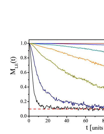
Figure 2: (Color Online). Time regimes of the local Loschmidt echo. Numerical results for a ring of 5 spins weakly coupled to another identical ring by an $XY$ interchain interaction ($\alpha=0$). The $M_{LE}$ is plotted as a function of the total evolution time $t=2t_{R}$. Notice that the stronger the interchain coupling $J_{\mathcal{SE}}$, the faster the saturation regime is reached (dashed line). From up to down, the different curves correspond to the coupling parameters $J_{\mathcal{SE}}$: $0.001,$ $0.01,$ $0.025,$ $0.05,$ $0.1,$ $0.25$ and $0.5$, in units of $J_{\mathcal{E}}$.

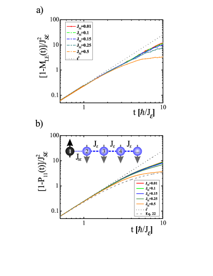
Figure 3: (Color online). a)Short time behavior of the Loschmidt Echo. The dotted line is the quadratic decay (Eq. 24). b)Short time behavior of the Survival Probability for an XY spin chain described by: $\hat{H}_{total}=J_{\mathcal{SE}}\left(\hat{S}_{1}^{+}\hat{S}_{2}^{-}+\hat{S}_{2}^{+}\hat{S}_{1}^{-}\right)+J_{\mathcal{E}}\sum_{n=2}^{\infty}\left(\hat{S}_{n}^{+}\hat{S}_{n+1}^{-}+\hat{S}_{n+1}^{+}\hat{S}_{n}^{-}\right)$, where the first spin is the system and the others constitute the environment. This system is known to satisfy the FGR Rufeil-Fiori and Pastawski (2006b). Notice the similarity between (a) and (b) in departing from the quadratic decay, which evinces the spreading time $t_{s}$. The dashed line shows a plot of Eq. 22 for $J_{\mathcal{SE}}=0.5J_{\mathcal{E}}$.

In Fig. 3-a the short time dynamics is compared with the expected quadratic decay (dotted line), which should appear in any quantum evolution at short times. Indeed, the plot of $\left(1-M_{LE}\right)/J_{\mathcal{SE}}^{2}$ (in log-log scale) as a function of time, shows that $M_{LE}$ follows a quadratic function:

$$M_{LE}(t)\simeq 1-[\frac{J_{\mathcal{SE}}}{2\hbar}]^{2}t^{2}.$$ (24)

This confirms that the short time decay is determined by $\sigma^{2}=(J_{\mathcal{SE}}/2\hbar)^{2}$, the second moment of the $\mathcal{SE}$ interaction. The agreement is observed until a time $t_{s}\simeq\hbar/J_{\mathcal{E}}$, which verifies the prediction for $t_{s}$ in terms of the $\mathcal{E}$ dynamics. For comparison, we show in Fig. 3-b the SP of an excitation in a single spin system $\mathcal{S}$ that interacts with the edge of a spin chain $\mathcal{E}$ where it can spread through pure $XY$ interactions. This model, shown in the inset, constitutes a paradigm for the onset of the FGR, because the DDCS is precisely defined by $N_{1}=1/J_{\mathcal{E}}$ and remains independent of $J_{\mathcal{SE}}$ Rufeil-Fiori and Pastawski (2006b). In Fig. 3-b, we also show with a dashed line the interpolative expression in Eq. 22, for the strongest coupling. This last expression deviates faster from the quadratic decay than the SP in the one-body chain.

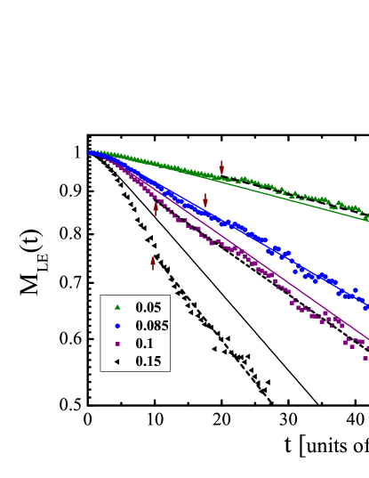
Figure 4: (Color online). The onset of the LE exponential decay. In the log scale, the dashed lines are the ideal exponentials determined by the fitting, show here for representative values. The delay in the entrance into the exponential regime is indicated with arrows pointing the first data used in the fitting. Continuous lines represent the interpolative Eq. 22, used with the corresponding $\sigma^{2}$ and $\Gamma$.

The onset of the exponential regime is exemplified in Fig. 4, for a few values of a pure XY $\mathcal{SE}$ interaction. As a general tendency, we observe that the asymptotic exponential decay only becomes well defined after some evolution period. We indicate with an arrow the initial data that we use to fit these rates. For comparison, the SP interpolative expression is plotted for the same decay rates. We notice that  for $J_{\mathcal{SE}}/J_{\mathcal{E}}\lesssim 0.085$ the interpolation starts to lie below the numerical results, and longer times are required to define the asymptotic exponential.

For long times, the LE shows a saturation plateau at $1/10$ (see Fig. 2). Such observation is consistent with the expectation that, within these coupling networks, the finite system of interacting spins behaves ergodically under the Loschmidt Echo dynamics, and thus the polarization spreads uniformly. At long times each site is polarized by the amount $1/(2m)$Ṫhe larger the coupling $J_{\mathcal{SE}}$, the faster the asymptotic saturation is reached.

In order to assess the exponential regime, we plot the characteristic rate $1/\tau_{\phi}$ in Fig. 5-a, as a function of $J_{\mathcal{SE}}^{2}$ in units of $J_{\mathcal{E}}/\hbar$. This quantity is appropriate to verify the FGR (Eq. 23), as long as $J_{\mathcal{SE}}^{2}$ is the typical scale for the second moment of the $\mathcal{S}$-$\mathcal{E}$ interaction and $1/J_{\mathcal{E}}$ that of $N_{1}$, the DDCS. We point out that rate calculations with longer rings and chains are seen to give similar values as long as the above parameters are kept the same. Such independence on $m$ resembles to the SP and LE for a single spin interacting with chains of different lengths Rufeil-Fiori and Pastawski (2006b); Dente et al. (2011). This is indicative that we are reaching the limit were the DDCS becomes dense enough to manifest the sum rule intrinsic to the FGRRufeil-Fiori and Pastawski (2009). Thus, we restrict our analysis to cases with $m=5$. Although several forms of the interchain Hamiltonians were considered by varying the anisotropy parameter $\alpha$ , we show only those relevant to NMR experiments: $XY$ ($\alpha=0$), isotropic ($\alpha=-\frac{1}{2}$), and truncated dipolar interaction ($\alpha=1$). We observe that the boundary conditions play a non-trivial role Danieli et al. (2004). For the case of open boundary conditions (Fig. 1-a), some oscillations appear mounted on a decay which also depend on the parity of $m,$ the number of spins in each chain. Here, we present only the results using closed boundary conditions (rings) where these effects are much weaker.

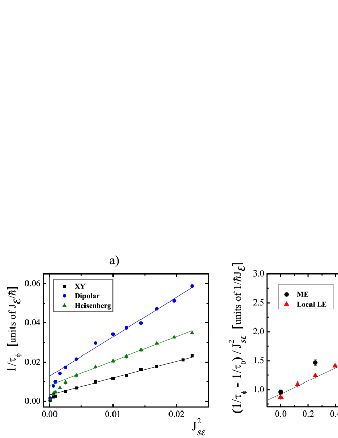
Figure 5: (Color Online). a) Decay rates for the NMR relevant interchain couplings, in units of $J_{\mathcal{E}}/\hbar$. The slopes and offsets depend on the value of $\alpha$, i.e. on the relative weight between the Ising (dephasing) and $XY$ (polarization transfer) contributions to the interchain coupling. b) Scaled rates showing the additivity of the XY and Ising contributions to the FGR rate as a function of $\alpha^{2}$. For comparison, the rates obtained from Mesoscopic Echo degradation data obtained in Ref. Álvarez et al. (2010c) are also plotted.

Note that the Loschmidt Echo allows one to explore a range of very weak perturbations yielding $\tau_{\phi}$ from the regime of exponential decay. Such a range was inaccessible in the interference contrast method Álvarez et al. (2010c). We observe that the rates in Fig. 5-a start from zero and have a rapid increase with the $J_{\mathcal{SE}}$ perturbation. After a small perturbation threshold the rates slow down to a linear dependence on the second moment of the perturbation. This confirms the validity of Eq. 23 for this range. The linear fit is shifted by an offset, $1/\tau_{0}$, which seems to depend on the nature of the $\mathcal{SE}$ interaction as it becomes larger for those perturbations with bigger Ising components.

Fig. 5-b shows the FGR contribution to the scaled decoherence rates $[1/\tau_{\phi}-1/\tau_{0}]/J_{\mathcal{SE}}^{2}$ as a function of interaction anisotropy $\alpha^{2}$. There, we also include the rates derived from the ME attenuation Álvarez et al. (2010c). From the slope in that plot we derive the contributions to the global decay rate $1/\tau_{\phi}$, arising from $XY$ and Ising processes in the interchain interaction:

$$\frac{1}{\tau_{\phi}}=\frac{1}{\tau_{0}}+\frac{1}{\tau_{\phi}^{XY}}+\frac{1}{\tau_{\phi}^{ZZ}}.$$ (25)

For the Loschmidt Echo results:

$$LE:~{}~{}~{}\frac{1}{\tau_{\phi}^{XY}}=(0.92\pm 0.04)\frac{J_{\mathcal{SE}}^{2}}{\hbar J_{\mathcal{E}}},$$ (26)

$$LE:~{}~{}~{}\frac{1}{\tau_{\phi}^{ZZ}}=(1.12\pm 0.04)\alpha^{2}\frac{J_{\mathcal{SE}}^{2}}{\hbar J_{\mathcal{E}}}.$$ (27)

In order to compare with the numerical results in Ref. Álvarez et al. (2010c), and translating its notation $-a/b\equiv 2\alpha$, the rates contributing to the ME degradation result:

$$ME:~{}~{}~{}\frac{1}{\tau_{\phi}^{XY}}=(1.00\pm 0.06)\frac{J_{\mathcal{SE}}^{2}}{\hbar J_{\mathcal{E}}},$$ (28)

$$ME:~{}~{}~{}\frac{1}{\tau_{\phi}^{ZZ}}=(2.0\pm 0.3)\alpha^{2}\frac{J_{\mathcal{SE}}^{2}}{\hbar J_{\mathcal{E}}}.$$ (29)

The most striking effect evinced by this comparison is that while the $XY$ contributions are essentially the same in both methods, the Ising contribution (i.e. pure dephasing) in the ME (Eq. 29) is almost twice the value obtained from the local LE. In the following section we analyze the origin of such result.

III.2 Analysis of the Decoherence Regimes

First, we would like to address the applicability of a “SP picture” for the LE in the present case, as it was proposed in Section II in connection with previous works. We verified that the short time decay is naturally ruled by the second moment of the $\mathcal{S}$-$\mathcal{E}$ interaction $\sigma^{2}=[J_{\mathcal{SE}}/2]^{2}$. We also checked the estimation for the spreading time $t_{s}\simeq\hbar/J_{\mathcal{E}}$, i.e. the transition from the quadratic short-time to the exponential regime. We found that such prediction is in agreement with the observed end of the quadratic decay.

In our spin problem, the LE exponential regime needs a further delay beyond $t_{s}$ to become well defined. This indicates that the DDCS, is not immediately defined but $J_{\mathcal{SE}}$ may have a role in its stabilization. Indeed, it is needed a back action of $J_{\mathcal{SE}}$ to break the strong degeneracy present in the unperturbed integrable $\mathcal{E}$, a finite $XY$ chain itself. Only then, one has the sufficiently dense spectrum required for the FGR to apply. Once the whole Hilbert space is made accessible by the perturbation, as many as $\tbinom{2m}{m}$ states become coupled by an interaction that conserves spin projection.

The interpolative Eq. 22 approximates satisfactorily the short-time decay, but it is not as well suited for intermediate times and certainly can not be applied to the saturation regime. These deviations can be, in principle, related to a failure in the SP picture to describe the local LE dynamics. The physics underlying Eq. 22 is based on the assumption of a sufficiently large number of particles and a well defined $N_{1}$. Also, one should be aware that our spin case is strictly finite, indeed quite small, and therefore the polarization cannot relax to zero. The observed asymptotic steady magnetization $1/2m$ can be identified with an ergodic behavior of the excitation described by the local LE dynamics. Since this ergodicity is not present in the unperturbed system, it should emerge as a consequence of the $\mathcal{SE}$ interaction.

It is important to notice that neither the rate obtained nor $\sigma^{2}$ depend on the total number of spins or on the number of spins in $\mathcal{S}$. The reason for such independence is related to the initial non-equilibrium condition stated in Eq. 6, which is a well localized excitation that maintains its character when it propagates through an $XY$ chain. It turns out that such localized excitation behaves much like a single particle and, in some sense, almost classically. This remains true at least when the LE is in the exponential regime. We have seen that the independence on the number of spins does not hold if one considers an initial state built-in as an arbitrary superposition. However, the investigation of this issue goes beyond the scope of the present study.

One should notice that splitting the FGR contribution to the decoherence rate into two well separated terms, a strategy also exploited in Ref. Álvarez et al. (2010c), evidences the additivity of the $XY$ and Ising processes. Each of them is associated with a different term in the interaction coupling $\hat{V}_{\mathcal{SE}}$ and require a different DDCS. These properties are indeed manifested in Fig. 5, that shows the linear dependence of $(1/\tau_{\phi}-1/\tau_{0})/J_{\mathcal{SE}}^{2}$ on the relative weight $\alpha^{2}$.

Comparing the rates obtained through the LE with those computed by the ME degradation Álvarez et al. (2010c), we notice that the $XY$ rates are equivalent and we can interpret such equivalence by using the mapping into a one-body evolution in both $\mathcal{S}$ and $\mathcal{E}$. Even when the one-body picture is not rigorously valid when the interaction $\hat{V}_{\mathcal{SE}}$ is turned on, it provides some physical insights Dente et al. (2011) that apply to more complex cases. Accordingly, the dynamics along the chains is only weakly affected by the tunnelling processes, (i.e. in a single particle picture, the kinetic energy along the chains commutes with that along the interchain direction). Thus, the rate $1/\tau_{\phi}^{XY}$ should coincide with the interchain tunnelling rate and we expect that it should not be affected by a time-reversal procedure within $\mathcal{S}$.

In contrast to the simple decay associated to the $XY$ component of the $\mathcal{S}$-$\mathcal{E}$ interaction, the Ising part causes energy fluctuations that induce a diffusion-like process within the system. This tends to blur out the dynamical recurrences (i.e. MEs). The smaller decoherence rate observed from the LE indicates that the time reversal procedure is at least partially effective to reverse such processes. In fact, the rates for the pure Ising interaction observed here from the LE are about half of those obtained from the ME Álvarez et al. (2010c). This means that the ME attenuation overestimates the phase degradation induced by the environment. As stated before, the displacement of a spin excitation in presence of a quenched spin environment plays the role of an Anderson disorder degrading the wave packet dynamics that produces the ME. Such degradation is computed as decoherence. The reversal of the internal $XY$ interaction would not be able to reverse such disorder. However, if the environment has an inner dynamics in a time scale comparable to that of the system ($J_{\mathcal{S}}\simeq{}J_{\mathcal{E}}$), there are particular fluctuations that allow for a perfect reversal of the system dynamics. Indeed, this occurs when both the hopping and the site energy signs are inverted. Such specific $\mathcal{E}$-fluctuations are those needed to unravel the phase shifts produced during the forward evolution. This argument, which relies on a single particle picture and equivalent time scales for the local dynamics in $\mathcal{S}$ and $\mathcal{E}$, is represented in Fig. 6. Thus, one may safely say that in the presence of a fluctuating environment, the LE is able to reconstruct the phases in an appreciable fraction of the local configurations.

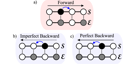
Figure 6: Spin propagation in presence of an Ising interchain interaction, represented as a single fermion moving through a binary alloy landscape. A filled circle is a spin up or a fermion, and an empty circle represents a spin down or a hole. All the processes are considered in the short time scale given by a single Trotter time step. a) Forward dynamics within the upper chain $\mathcal{S}$, in presence of the ”random site energies” produced by the Ising interaction with the lower chain $\mathcal{E}$. b) If $\mathcal{E}$ remains frozen, the backward evolution in $\mathcal{S}$ is imperfect because the signs of the “site energies” are not inverted. c)A particular evolution of $\mathcal{E}$ provides a perfectly reversed dynamics for $\mathcal{S}$. In this case, the local portion of potential landscape, that determined the excitation’s forward evolution, is reversed.

IV CONCLUSIONS

We presented an evaluation of decoherence for a spin chain in realistic many-body scenarios. As specific realizations for structured environments, we used a second spin chain weakly coupled to the first. This system-environment interaction ranges from pure $XY$ to truncated dipolar, passing through the isotropic Heisenberg interaction. In order to evaluate decoherence, we resorted to the Loschmidt Echo, which here is the local polarization recovered after an imperfect time reversal procedure. The attenuation of such echoes yields a first hand estimation of the decoherence rate, without any ad-hoc assumptions about spectral functions Chakravarty and Leggett (1984); Weiss (2008) or stochastic noise operators Blanchard et al. (1994); Machida et al. (1999). Our computational technique involves a Trotter Suzuki decomposition assisted by a recently developed algorithm that relies on quantum parallelism to evaluate local observables Álvarez et al. (2008).

In the present many-body context, the decoherence rate is separated in two contributions, both of which scale with $J_{\mathcal{SE}}^{2}$ and $1/J_{\mathcal{E}}$, i.e. as a Fermi golden rule. The rates obtained here do not depend on the number $m$ of spins. This is strongly related to the localized initial condition but such independence does not hold if the initial condition is a superposition state. It is also indicative of a specific sum rule relating the local second moment of the interaction and the DDCS, which in this many-body case coincides with that resulting from a single particle picture.

In the adopted model, the close connection between the Loschmidt Echo and the Survival Probability allows for a comparison with the expectancies of the last magnitude. In particular, we assessed an interpolative formula Flambaum and Izrailev (2001) that matches the initial quadratic decay with the exponential regime. Despite of the qualitative agreement, the Loschmidt Echo evidences a richer and more complex dynamical behavior than those predictions. For instance, the breakdown of single-particle degeneracies due to the $\mathcal{S}$-$\mathcal{E}$ interaction and the appearance of an ergodic regime, manifested as a steady saturation, are now clearly shown in the numerical results.

The numerical studies performed here confirm that the Loschmidt Echo is better to quantify decoherence than the standard analysis based on interference degradation, as it recovers information that escaped such analysis Álvarez et al. (2010c). Additionally, by compensating the intrinsic dynamical interferences of the system through time reversal, the LE gets rid of most of the trivial part in the $\mathcal{S}$ dynamics that conceals the decoherence effects. Thus the LE provides a smooth and continuous access to characterize decoherence processes.

V Acknowledgements

We acknowledge Fernando Pastawski for critical comments on an initial version of this manuscript as well as Gonzalo Usaj and Greg Boutis for lively discussions. This work was performed with the financial support from CONICET, ANPCyT, SeCyT-UNC, MinCyT-Cor, and NVIDIA professor partnership program.

Appendix A The spin autocorrelation function.

We show here equivalent expressions for the spin autocorrelation expressed in Eq. 5. The autocorrelation $P_{1,1}(t)$ gives the local polarization at time $t$ along the $z$ direction in site $1$ provided that at time $t=0$ the system was in its thermal equilibrium state plus a local excitation in site $1$. In order to show this assertion explicitly, we rewrite the numerator in Eq. 5:

$$\left\langle\Psi_{eq}\right|\hat{S}_{1}^{z}(t)\hat{S}_{1}^{z}(0)\left|\Psi_{eq}\right\rangle=\left\langle\Psi_{eq}\right|\left(\hat{S}_{1}^{+}(t)\hat{S}_{1}^{-}(t)-\frac{1}{2}\right)\left(\hat{S}_{1}^{+}(0)\hat{S}_{1}^{-}(0)-\frac{1}{2}\right)\left|\Psi_{eq}\right\rangle,$$ (30)

where we have used the identity $\hat{S}^{z}=\hat{S}^{+}\hat{S}^{-}-\frac{1}{2}$, which is valid for spins $1/2$. The $\mathcal{S}$ label has been dropped for simplicity. Then,

$$\left\langle\Psi_{eq}\right|\hat{S}_{1}^{z}(t)\hat{S}_{1}^{z}(0)\left|\Psi_{eq}\right\rangle=\left\langle\Psi_{eq}\right|\hat{S}_{1}^{+}(t)\hat{S}_{1}^{-}(t)\hat{S}_{1}^{+}(0)\hat{S}_{1}^{-}(0)\left|\Psi_{eq}\right\rangle-\frac{1}{4},$$ (31)

where we have rearranged the terms and used the high temperature hypothesis for $\left|\Psi_{eq}\right\rangle$ explicitly, i.e. $\left\langle\Psi_{eq}\right|\hat{S}_{1}^{z}(t)\left|\Psi_{eq}\right\rangle=\left\langle\Psi_{eq}\right|\hat{S}_{1}^{z}(0)\left|\Psi_{eq}\right\rangle=0$. It is crucial now to identify the meaning of the expectation value $\left\langle\Psi_{eq}\right|\cdots\left|\Psi_{eq}\right\rangle$ as a trace over the basis states (see Eq. (3) in Ref. Danieli et al. (2004)). Hence, the invariance of the trace under cyclic permutation leads to:

$$\left\langle\Psi_{eq}\right|\hat{S}_{1}^{z}(t)\hat{S}_{1}^{z}(0)\left|\Psi_{eq}\right\rangle=\left\langle\Psi_{eq}\right|\hat{S}_{1}^{-}(0)\hat{S}_{1}^{+}(t)\hat{S}_{1}^{-}(t)\hat{S}_{1}^{+}(0)\left|\Psi_{eq}\right\rangle-\frac{1}{4},$$ (32)

and one identifies the non-equilibrium initial condition $\hat{S}_{1}^{+}(0)\left|\Psi_{eq}\right\rangle$, which after normalization yields exactly Eq. 6:

$$\left|\Psi_{ne}\right\rangle=\frac{\hat{S}_{\mathcal{S},1}^{+}\left|\Psi_{eq}\right\rangle}{\left|\left\langle\Psi_{eq}\right|\hat{S}_{\mathcal{S},1}^{-}\hat{S}_{\mathcal{S},1}^{+}\left|\Psi_{eq}\right\rangle\right|^{1/2}}.$$ (33)

Accordingly, the numerator can be written as:

$$\left\langle\Psi_{eq}\right|\hat{S}_{1}^{z}(t)\hat{S}_{1}^{z}(0)\left|\Psi_{eq}\right\rangle =\left|\left\langle\Psi_{eq}\right|\hat{S}_{\mathcal{S},1}^{-}\hat{S}_{\mathcal{S},1}^{+}\left|\Psi_{eq}\right\rangle\right|\left\langle\Psi_{neq}\right|\hat{S}_{1}^{+}(t)\hat{S}_{1}^{-}(t)\left|\Psi_{neq}\right\rangle-\frac{1}{4},$$

$$=\frac{1}{2}\left\langle\Psi_{ne}\right|\hat{S}_{1}^{+}(t)\hat{S}_{1}^{-}(t)\left|\Psi_{ne}\right\rangle-\frac{1}{4}.$$ (34)

The denominator in Eq. 5 is $\left\langle\Psi_{eq}\right|\hat{S}_{1}^{z}(0)\hat{S}_{1}^{z}(0)\left|\Psi_{eq}\right\rangle\equiv\frac{1}{4}$. Therefore,

$$P_{1,1}(t)=2\left\langle\Psi_{ne}\right|\hat{S}_{1}^{+}(t)\hat{S}_{1}^{-}(t)\left|\Psi_{ne}\right\rangle-1.$$ (35)

In the Schrödinger picture it yields:

$$P_{1,1}(t) =2\left\langle\Psi_{ne}\right|e^{\mathrm{i}\hat{H}_{total}t/\hbar}\hat{S}_{1}^{+}\hat{S}_{1}^{-}e^{-\mathrm{i}\hat{H}_{total}t/\hbar}\left|\Psi_{ne}\right\rangle-1,$$ (36)

$$P_{1,1}(t) =2\left\langle\Psi_{ne}\right|e^{\mathrm{i}\hat{H}_{total}t/\hbar}\left(\hat{S}_{1}^{+}\hat{S}_{1}^{-}-\frac{1}{2}\right)e^{-\mathrm{i}\hat{H}_{total}t/\hbar}\left|\Psi_{ne}\right\rangle,$$ (37)

$$P_{1,1}(t) =2\left\langle\Psi_{ne}\right|e^{\mathrm{i}\hat{H}_{total}t/\hbar}\hat{S}_{1}^{z}e^{-\mathrm{i}\hat{H}_{total}t/\hbar}\left|\Psi_{ne}\right\rangle.$$ (38)

Thus, the autocorrelation $P_{1,1}(t)$ written in the form of Eq. 38 is, in fact, the expectation value of the $\hat{S}_{1}^{z}$ operator over the evolved non-equilibrium state $e^{-\mathrm{i}\hat{H}_{total}t/\hbar}\left|\Psi_{ne}\right\rangle$. We note that an equivalent reasoning can be performed in the case of the local Loschmidt Echo in Eq. 15 just replacing the forward propagator $e^{-\mathrm{i}\hat{H}_{total}t/\hbar}$ by the Loschmidt Echo propagator $e^{-\tfrac{\mathrm{i}}{\hbar}(-\hat{H}_{\mathcal{S}}+\hat{\Sigma})t_{R}}e^{-\tfrac{\mathrm{i}}{\hbar}(\hat{H}_{\mathcal{S}}+\hat{\Sigma})t_{R}}$.

Appendix B Numerical Simulations with Trotter-Suzuki evolutions.

The computation of the time dependent observable in Eq. 5 requires to evolve each of the states participating in the ensemble. However, its implementation for large systems, e.g. by means of a $4^{th}$ order Trotter-Suzuki decomposition Rieth and Schommers (2006), soon becomes quite expensive in computational resources. Instead, the local nature of the excitation allows the employment of an algorithm exploiting the quantum parallelism Álvarez et al. (2008) to give an exponential reduction of computational efforts. The evolution of a few pure states is enough to describe the ensemble averaged excitation dynamics. Thus, a typical initial state representing the whole ensemble has the form:

$$\left|\Psi\right\rangle=\left|\uparrow_{1}\right\rangle\otimes\left\{{\displaystyle\sum\limits_{r=1}^{2^{2m-1}}}\frac{1}{\sqrt{2^{2m-1}}}e^{\mathrm{i}\varphi_{r}}\text{\ }\left|\beta_{r}\right\rangle\right\},\text{ \ \ \ }\varphi_{r}=\text{random phase,}$$ (39)

which exploits the quantum superposition over the whole spin set. Typically, a few of these entangled states is enough to get rid of statistical noise and obtain local physical observables with good accuracy. This highly efficient technique for spin-ensemble calculations is enhanced by the parallelization enabled by its implementation on a General Purpose Graphical Processing Unit (GPGPU).

References

- Bennett and DiVincenzo (2000) C. H. Bennett and D. P. DiVincenzo, Nature 404, 247 (2000).
- Awschalom and Flatté (2007) D. D. Awschalom and M. E. Flatté, Nat. Phys. 3, 153 (2007).
- Bloch et al. (2008) I. Bloch, J. Dalibard, and W. Zwerger, Rev. Mod. Phys. 80, 885 (2008), arXiv:0704.3011 .
- Sherson et al. (2010) J. F. Sherson, C. Weitenberg, M. Endres, M. Cheneau, I. Bloch, and S. Kuhr, Nature 467, 68 (2010), arXiv:1006.3799 [cond-mat.quant-gas] .
- Dicarlo et al. (2010) L. Dicarlo, M. D. Reed, L. Sun, B. R. Johnson, J. M. Chow, J. M. Gambetta, L. Frunzio, S. M. Girvin, M. H. Devoret, and R. J. Schoelkopf, Nature 467, 574 (2010), arXiv:1004.4324 [cond-mat.mes-hall] .
- Grinolds et al. (2011) M. S. Grinolds, P. Maletinsky, S. Hong, M. D. Lukin, R. L. Walsworth, and A. Yacoby, Nat. Phys. 467, 68 (2011), arXiv:1103.0546 [cond-mat.mes-hall] .
- Levstein et al. (1998) P. R. Levstein, G. Usaj, and H. M. Pastawski, J. Chem. Phys. 108, 2718 (1998).
- Pastawski et al. (2000) H. M. Pastawski, P. R. Levstein, G. Usaj, J. Raya, and J. Hirschinger, Physica A 283, 166 (2000).
- Krojanski and Suter (2004) H. G. Krojanski and D. Suter, Phys. Rev. Lett. 93, 090501 (2004).
- Zurek et al. (2007) W. H. Zurek, F. M. Cucchietti, and J. P. Paz, Acta Phys. Pol. B 38, 1685 (2007), and references therein, arXiv:quant-ph/0611200 .
- Kosut et al. (2008) R. L. Kosut, A. Shabani, and D. A. Lidar, Phys. Rev. Lett. 100, 020502 (2008).
- Knill and Laflamme (1997) E. Knill and R. Laflamme, Phys. Rev. A 55, 900 (1997).
- Viola et al. (1999) L. Viola, E. Knill, and S. Lloyd, Phys. Rev. Lett. 82, 2417 (1999).
- Ryan et al. (2010) C. A. Ryan, J. S. Hodges, and D. G. Cory, Phys. Rev. Lett. 105, 200402 (2010), and references therein.
- Álvarez et al. (2010a) G. A. Álvarez, A. Ajoy, X. Peng, and D. Suter, Phys. Rev. A 82, 042306 (2010a).
- Ladd et al. (2010) T. D. Ladd, F. Jelezko, R. Laflamme, Y. Nakamura, C. Monroe, and J. L. O’Brien, Nature 464, 45 (2010), arXiv:1009.2267 [quant-ph] .
- Bose (2003) S. Bose, Phys. Rev. Lett. 91, 207901 (2003).
- Mádi et al. (1997) Z. L. Mádi, B. Brutscher, T. Schulte-Herbrüggen, R. Brüschweiler, and R. R. Ernst, Chem. Phys. Lett. 268, 300 (1997).
- Cappellaro et al. (2007) P. Cappellaro, C. Ramanathan, and D. G. Cory, Phys. Rev. A 76, 032317 (2007).
- Zhang et al. (2009) W. Zhang, P. Cappellaro, N. Antler, B. Pepper, D. G. Cory, V. V. Dobrovitski, C. Ramanathan, and L. Viola, Phys. Rev. A 80, 052323 (2009), arXiv:0906.2434 [quant-ph] .
- Rufeil-Fiori et al. (2009) E. Rufeil-Fiori, C. M. Sánchez, F. Y. Oliva, H. M. Pastawski, and P. R. Levstein, Phys. Rev. A 79, 032324 (2009).
- Fel’dman and Lacelle (1997) E. B. Fel’dman and S. Lacelle, J. Chem. Phys. 107, 7067 (1997).
- Doronin et al. (2000) S. Doronin, I. Maksimov, and E. Fel’dman, J. Experiment. Theoret. Phys. 91, 597 (2000), 10.1134/1.1320096.
- Doronin and Fel’dman (2005) S. I. Doronin and E. B. Fel’dman, Solid State Nucl. Mag. 28, 111 (2005).
- Ramanathan et al. (2011) C. Ramanathan, P. Cappellaro, L. Viola, and D. G. Cory, New J. Phys. 13, 103015 (2011).
- Álvarez et al. (2010b) G. A. Álvarez, M. Mishkovsky, E. P. Danieli, P. R. Levstein, H. M. Pastawski, and L. Frydman, Phys. Rev. A 81, 060302 (2010b).
- Cappellaro et al. (2011) P. Cappellaro, L. Viola, and C. Ramanathan, Phys. Rev. A 83, 032304 (2011), arXiv:1011.0736 [quant-ph] .
- Pastawski et al. (1995) H. M. Pastawski, P. R. Levstein, and G. Usaj, Phys. Rev. Lett. 75, 4310 (1995).
- Pastawski (1996) H. Pastawski, Chem. Phys. Lett. 261, 329 (1996), arXiv:cond-mat/9609036 .
- Prigodin et al. (1994) V. N. Prigodin, B. L. Altshuler, K. B. Efetov, and S. Iida, Phys. Rev. Lett. 72, 546 (1994).
- Álvarez et al. (2010c) G. A. Álvarez, E. P. Danieli, P. R. Levstein, and H. M. Pastawski, Phys. Rev. A 82, 012310 (2010c).
- Jalabert and Pastawski (2001) R. A. Jalabert and H. M. Pastawski, Phys. Rev. Lett. 86, 2490 (2001).
- Sánchez et al. (2009) C. M. Sánchez, P. R. Levstein, R. H. Acosta, and A. K. Chattah, Phys. Rev. A 80, 012328 (2009).
- Andersen et al. (2006) M. F. Andersen, A. Kaplan, T. Grünzweig, and N. Davidson, Phys. Rev. Lett. 97, 104102 (2006).
- Schäfer et al. (2005) R. Schäfer, H.-J. Stöckmann, T. Gorin, and T. H. Seligman, Phys. Rev. Lett. 95, 184102 (2005).
- Jacquod and Petitjean (2009) P. Jacquod and C. Petitjean, Adv. in Phys. 58, 67 (2009).
- Gorin et al. (2006) T. Gorin, T. Prosen, T. H. Seligman, and M. Znidaric, Phys. Rep. 435, 33 (2006).
- Goussev et al. (2012) A. Goussev, R. A. Jalabert, H. M. Pastawski, and D. Wisniacki, ArXiv e-prints (2012), arXiv:1206.6348 [nlin.CD] .
- Flambaum and Izrailev (2001) V. V. Flambaum and F. M. Izrailev, Phys. Rev. E 64, 026124 (2001).
- Levstein et al. (1991) P. R. Levstein, H. M. Pastawski, and R. Calvo, J. Phys.: Condens. Matter 3, 1877 (1991).
- Zhang et al. (1992) S. Zhang, B. H. Meier, and R. R. Ernst, Phys. Rev. Lett. 69, 2149 (1992).
- Danieli et al. (2004) E. P. Danieli, H. M. Pastawski, and P. R. Levstein, Chem. Phys. Lett. 384, 306 (2004).
- Abragam (1986) A. Abragam, The principles of nuclear magnetism, The International Series on Monographs on physics (Oxford University Press, Oxford, 1986).
- Slichter (1980) C. P. Slichter, Principles of magnetic resonance; 2nd ed., Springer series in solid state sciences (Springer, Berlin, 1980).
- Rieth and Schommers (2006) M. Rieth and W. Schommers, Handbook of Theoretical and Computational Nanotechnology: Quantum and molecular computing, quantum simulations, Nanotechnology book series (American Scientific Publishers, 2006).
- Álvarez et al. (2008) G. A. Álvarez, E. P. Danieli, P. R. Levstein, and H. M. Pastawski, Phys. Rev. Lett. 101, 120503 (2008).
- Lieb et al. (1961) E. Lieb, T. Schultz, and D. Mattis, Ann. Phys. 16, 407 (1961).
- Danieli et al. (2005) E. P. Danieli, H. M. Pastawski, and G. A. Álvarez, Chem. Phys. Lett. 402, 88 (2005).
- Khitrin and Fung (1999) A. K. Khitrin and B. M. Fung, J. Chem. Phys. 111, 7480 (1999).
- Anderson (1978) P. W. Anderson, Rev. Mod. Phys. 50, 191 (1978).
- Petitjean and Jacquod (2006) C. Petitjean and P. Jacquod, Phys. Rev. Lett. 97, 124103 (2006).
- Bohigas and Flores (1971) O. Bohigas and J. Flores, Phys. Lett. B 34, 261 (1971).
- Flambaum et al. (1996) V. V. Flambaum, G. F. Gribakin, and F. M. Izrailev, Phys. Rev. E 53, 5729 (1996).
- Flambaum and Izrailev (1997) V. V. Flambaum and F. M. Izrailev, Phys. Rev. E 55, R13 (1997).
- Jacquod and Shepelyansky (1997) P. Jacquod and D. L. Shepelyansky, Phys. Rev. Lett. 79, 1837 (1997).
- Georgeot and Shepelyansky (1998) B. Georgeot and D. L. Shepelyansky, Phys. Rev. Lett. 81, 5129 (1998).
- Santos et al. (2012) L. F. Santos, F. Borgonovi, and F. M. Izrailev, Phys. Rev. Lett. 108, 094102 (2012).
- Flambaum and Izrailev (2000) V. V. Flambaum and F. M. Izrailev, Phys. Rev. E 61, 2539 (2000).
- Rufeil-Fiori and Pastawski (2009) E. Rufeil-Fiori and H. M. Pastawski, Physica B 404, 2812 (2009), arXiv:0812.1009 [quant-ph] .
- Rufeil-Fiori and Pastawski (2006a) E. Rufeil-Fiori and H. M. Pastawski, Braz. J. Phys. 36, 844 (2006a).
- Jacquod et al. (2001) P. Jacquod, P. Silvestrov, and C. Beenakker, Phys. Rev. E 64, 055203 (2001).
- Cucchietti et al. (2006) F. M. Cucchietti, C. H. Lewenkopf, and H. M. Pastawski, Phys. Rev. E 74, 026207 (2006).
- Rufeil-Fiori and Pastawski (2006b) E. Rufeil-Fiori and H. M. Pastawski, Chem. Phys. Lett. 420, 35 (2006b).
- Dente et al. (2011) A. D. Dente, P. R. Zangara, and H. M. Pastawski, Phys. Rev. A 84, 042104 (2011).
- Chakravarty and Leggett (1984) S. Chakravarty and A. J. Leggett, Phys. Rev. Lett. 52, 5 (1984).
- Weiss (2008) U. Weiss, Quantum dissipative systems, Series in modern condensed matter physics (World Scientific, Singapore, 2008).
- Blanchard et al. (1994) P. Blanchard, G. Bolz, M. Cini, G. F. de Angelis, and M. Serva, J. Stat. Phys. 75, 749 (1994).
- Machida et al. (1999) K. Machida, H. Nakazato, S. Pascazio, H. Rauch, and S. Yu, Phys. Rev. A 60, 3448 (1999), arXiv:quant-ph/9903009 .