FITSH – a software package for image processing

Abstract

In this paper we describe the main features of the software package named FITSH, intended to provide a standalone environment for analysis of data acquired by imaging astronomical detectors. The package provides utilities both for the full pipeline of subsequent related data processing steps (incl. image calibration, astrometry, source identification, photometry, differential analysis, low-level arithmetic operations, multiple image combinations, spatial transformations and interpolations, etc.) and for aiding the interpretation of the (mainly photometric and/or astrometric) results. The package also features a consistent implementation of photometry based on image subtraction, point spread function fitting and aperture photometry and provides easy-to-use interfaces for comparisons and for picking the most suitable method for a particular problem. This set of utilities found in the package are built on the top of the commonly used UNIX/POSIX shells (hence the name of the package), therefore both frequently used and well-documented tools for such environments can be exploited and managing massive amount of data is rather convenient.

1 Introduction

In general, homogeneous data acquisition and subsequent data processing are essential for obtaining a proper measurement and characterize various observations. It is especially true for observing weak signals and analyzing related data series with a relatively low signal-to-noise (S/N) ratio. These mentioned data processing steps include a) calibration and per-pixel arithmetic operations; b) source detection, source profile characterization and (optionally space-varying) PSF determination; c) catalogue and cross-matching, coordinate list processing and astrometry; d) image registration, convolution and combination of multiple images; e) instrumental photometry (normal, PSF fitting and based on image subtraction); f) refined profile modelling, obtaining centroid and shape parameters; g) creation of model and artificial images; h) data modelling and regression analysis. Although several software solutions exist for processing imaging astronomical data (see e.g. IRAF, ISIS, SExtractor, utilities and wrappers around these implemented in Python or IDL), we intended to develop a lightweight package that is both a versatile solution for astronomical image processing (focusing mostly on the processing of optical imaging data) and features the many of the most recent data analysis and interpretation algorithms.

This paper presents a software package named FITSH, that provides a set of independent binary programs (called “tasks”) that are designed to be executed from a UNIX command line shell or shell script. Each of these tasks performs a specific operation (see the various steps above), while the details of a certain operation are specified via command line switches and/or arguments. Therefore this package does not need any higher level operating environment than a standard UNIX shell, however, processing the related data might require a little more knowledge of the used shell itself (the documentation and available examples use the bash shell). Additionally, some of the processing steps might require minor or basic operations performed with other tools like awk or text processing utilities (sort, uniq, paste, …). Another advantage of a “plain” UNIX environment is the option for exploiting other shell-level features, such as very easy implementation of remote execution, job control, batched processing (including background processing), higher level ways of run tasks in parallel, and integration for autonomous observing systems

In order to have a consistent implementation of the procedures required by astronomical image processing, several well known algorithms (that are ultimately used as standard procedures) have also been implemented in the FITSH package. The details of these are known from the literature. These include image preprocessing and calibration (Chromey, 2010), basic source extraction, aperture photometry and PSF modelling (Stetson, 1987, 1989) or differential image analysis (Alard & Lupton, 1998). The new improvements, including routines related to astrometry and catalogue matching, image transformations, consistent photometry on subtracted (differential) images, various regression analysis methods, etc. have been discussed in more details in Pál (2009b). See this work and references therein for more details. In this paper we also refer to some parts of that thesis during the discussion of various tasks.

The structure of this paper goes as follows. Sec. 2 describes briefly some aspects of the practical implementation. In Sec. 3, each of the main tasks are described in more detail, featuring small “script-lets” as a demonstration of the syntax of the various tasks. In Sec. 4, we summarize the results. The software package has its own website located at http://fitsh.szofi.net. This site displays information about the program and the tasks (including documentation and detailed examples), it is the primary download source of the package itself, and additionally, serves a public forum for the program users in various topics.

2 Implementation aspects

Table 1: An overview of the standalone tasks included in the package, displaying their main purposes and the types of input and output data.

Task	Main purpose	Type of input	Type of output
fiarith	Evaluates arithmetic expressions on images as operands.	A set of FITS images.	A single FITS image.
ficalib	Performs various calibration steps on the input images.	A set of raw FITS images.	A set of calibrated FITS images.
ficombine	Combines (most frequently averages) a set of images.	A set of FITS images.	A single FITS image.
ficonv	Obtains an optimal convolution transformation between two images or use an existing convolution transformation to convolve an image.	Two FITS images or a single image and a transformation.	A convolution transformation or a single image.
fiheader	Manipulates, i.e. reads, sets, alters or removes some FITS header keywords and/or their values.	A single FITS image (alternation) or more FITS images (if header contents are just read).	A FITS image with altered header or a series of keywords/values from the headers.
fiign	Performs low-level manipulations on masks associated to FITS images.	A single FITS image (with some optional mask).	A single FITS image (with an altered mask).
fiinfo	Gives some information about the FITS image in a human-readable form or creates image stamps in a conventional format.	A single FITS image.	Basic information or PNM images.
fiphot	Performs photometry on normal, convolved or subtracted images.	A single FITS image (with additional reference photometric information if the image is a subtracted one).	Instrumental photometric data.
firandom	Generates artificial object lists and/or artificial (astronomical) images.	List of sources to be drawn to the image or an arithmetic expression that describes how the list of sources is to be created.	List of sources and/or a single FITS image.
fistar	Detects and characterizes point-like sources from astronomical images.	A single FITS image.	List of detected sources and an optional PSF image (in FITS format).
fitrans	Performs generic geometric (spatial) transformations on the input image.	A single FITS image.	A single, transformed FITS image.
fi[un]zip	Compresses and decompresses primary FITS images.	A single uncompressed or compressed FITS image file.	A single compressed or uncompressed FITS image file.
grcollect	Performs data transposition on the input tabulated data or do some sort of statistics on the input data.	A set of files containing tabulated data.	A set of files containing the transposed tabulated data or a single file for the statistics, also in a tabulated form.
grmatch	Matches lines read from two input files of tabulated data, using various criteria (point matching, coordinate matching or identifier matching).	Two files containing tabulated data (that must be two point sets in the case of point or coordinate matching).	One file containing the matched lines and in the case of point matching, an additional file that describes the best fit geometric transformation between the two point sets.
grselect	Selects lines from tabulated data using various criteria.	A single file containing tabulated data.	The filtered rows from the input data.
grtrans	Transforms a single coordinate list or derives a best-fit transformation between two coordinate lists.	A single file containing a coordinate list and a file that describes the transformation or two files, each one is containing a coordinate list.	A file with the transformed coordinate list in tabulated from or a file that contains the best-fit transformation.
lfit	General purpose arithmetic evaluation, regression and data analysis tool.	Files containing data to be analyzed in a tabulated form.	Regression parameters or results of the arithmetic evaluation.

This section briefly summarize the main aspects of the implementation of the package tasks. The tasks can be divided into two well separated groups with respect to the main purposes. In the first group there are the programs that manipulate the (astronomical) images themselves (for instance, read an image, generate one or do a specific transformation on a single image or on more images). In the second group, there are the tasks that manipulate textual data, mostly numerical data presented in a tabulated form.

In general, all of these tasks are capable to the following.

2.1 Logging and versions

The codes give release and version information as well as the invocation can be logged on demand. The version information can be reported by a single call of the given task, moreover it is logged along with the invocation arguments in the form of special FITS keywords (if the main output of the actual code is a processed FITS image) and/or in the form of textual comments (if the main output of the code is text data). Preserving the version information along with the invocation arguments makes any kind of output easily reproducible.

2.2 Pipelines

All of the tasks are capable to read their input from stdin (the standard input on UNIX environments) and write the results to stdout (the UNIX standard output). Since many of these tasks manipulate relatively large amount of data, the number of unnecessary hard disk operations can therefore be reduced as small as possible. Moreover, in many cases the output of one of the programs is the input of the another one: pipes, available in all of the modern UNIX-like operating systems, are basically designed to perform such bindings between the (standard) output and (standard) input of two programs. Therefore, such a capability of redirecting the input/output data streams significantly reduce the overhead of background storage operations.

2.3 Symbolic operations

For the tasks dealing with symbolic operations and functions, a general back-end library is provided to make a user-friendly interface to specify arithmetic expressions. This kind of approach in software systems is barely used, since such a symbolic specification of arithmetic expressions does not provide a standalone language. However, it allows an easy and transparent way for arbitrary operations, and turned out to be very efficient in higher level data reduction scripts.

2.4 Extensions

Tasks that manipulate FITS images are capable to handle files with multiple extensions. The FITS standard allows the user to store multiple individual images, as well as (ASCII or binary) tabulated data in a single file. The control software of some detectors produces images that are stored in this extended format. Other kind of detectors (which acquire individual images with a very short exposure time) might store the data in the three dimensional format called “data cube”. The tasks are also capable to process such data storage formats.

The list of standalone tasks and their main purposes that come with the package are shown in Table 1. The next section discusses these tasks in more details.

3 Tasks

In this section we summarize the features and properties each of the standalone tasks that are implemented as distinct binary executables.

3.1 Basic operations on FITS headers and keywords – fiheader

The main purpose of the fiheader utility is to read specific values from the headers of FITS files and/or alter them on demand.

Although most of the information about the observational conditions is stored in the form of FITS keywords, image manipulation programs use only the necessary ones and most of the image processing parameters are passed as command line arguments (such keywords and data are, for example, the gain, the image centroid coordinates, astrometrical solutions). The main reasons why this kind of approach was chosen are the following.

• First, interpreting many of the standard keywords leads to false information about the image in the cases of wide-field or heavily distorted images. Such a parameter is the gain that can be highly inhomogeneous for images acquired by an optical system with non-negligible vignetting and the gain itself cannot be described by a single real number, rather a polynomial or some equivalent function. Similarly, the standard World Coordinate System information, describing the astrometrical solution of the image, has been designed for small field-of-view images, i.e. the number of coefficients are insufficiently few to properly constrain the astrometry of a distorted image.

• Second, altering the meanings of standard keywords leads to incompatibilities with existing software. For example, if the format of the keyword GAIN was changed to be a string of finite real numbers (describing a spatially varied gain), other programs would not be able to parse this redefined keyword.

Therefore, our conclusion was not altering the syntax of the existing keywords, but to define some new (wherever it was necessary). The fiheader utility enables the user to read any of the keywords, and allows higher level scripts to interpret the values read from the headers and pass their values to other programs in the form of command line arguments.

3.2 Basic arithmetic operations on images – fiarith

The task fiarith allows the user to perform simple operations on one or more astronomical images. Supposing all of the input images have the same size, the task allows the user to do per pixel arithmetic operations as well as manipulations depend on the pixel coordinates themselves. Unlike utilities like imarith in IRAF, fiarith is capable to process both the symbolic arithmetic operations (done via the libpsn library, see Sec. 2.3) and the per-pixel operations via a single call.

3.3 Basic information about images – fiinfo

The aim of the task fiinfo is twofold. First, this task is capable to gather some statistics and masking information of the image. These include

• general statistics, such as mean, median, minimum, maximum, standard deviation of the pixel values;

• statistics derived after rejecting the outlier pixels;

• estimations for the background level and its spatial variations;

• estimations for the background noise; and

• the number of masked pixels, detailing for all occurring mask types.

The most common usage of fiinfo in this statistical mode is to deselect those calibration frames that seem to be faulty (e.g. saturated sky flats, aborted images or so).

Second, the task is capable to convert astronomical images into widely used graphics file formats. Almost all of the scaling options available in the well known DS9 program (see Joye & Mandel, 2003) have been implemented in fiinfo, moreover, the user can define arbitrary color palettes as well. In practice, fiinfo creates only images in PNM (portable anymap) format. Images stored in this format can then be converted to any of the widely used graphics file formats (such as JPEG, PNG), using existing software (e.g. netpbm, convert/ImageMagick). Figures in this paper displaying stamps from real (or mock) astronomical images have also been created using this mode of the task.

3.4 Combination of images – ficombine

The main purpose of image combination is either to create a single image with from individual images (mainly in order to create higher signal-to-noise ratio frames and/or images with smaller statistical noise) or create a mosaic image covering a larger area (mainly from images with smaller field-of-view). The task ficombine is intended to perform this averaging of individual images. This task has several possible applications in a data reduction pipeline. For instance, it is used to create the master calibration frames (see also Sec. 3.5) or the reference frame required by the method of image subtraction is also created by averaging individual registered object frames (see also Sec. 3.11 about the details of image registration).

In the actual implementation, such combination is employed as a per pixel averaging, where the method of averaging and its fine tune parameters can be specified via command line arguments. The most frequently used “average values” are the mean and median values. In many applications, rejection of outlier values are required, for instance, omitting pixels affected by cosmic ray events. The respective parameters for tuning the outlier rejection are also given as command line options. See Sec. 3.5 for an example about the usage of ficombine, demonstrating its usage in a simple implementation of a calibration pipeline.

       #!/bin/sh
      
# Names of the individual files storing the raw bias, dark, flat and object frames:
BIASLIST=($SOURCE/bias-*.fits)
DARKLIST=($SOURCE/dark-*.fits)
FLATLIST=($SOURCE/flat-*.fits)
IOBJLIST=($SOURCE/target_object-*.fits)
      
# Calibrated images: all the images have the same name but put into a separate directory ($TARGET):
R_BIASLIST=($(for f in "${BIASLIST[*]}" ; do echo $TMP/bias/‘basename $f‘ ; done))
R_DARKLIST=($(for f in "${DARKLIST[*]}" ; do echo $TMP/dark/‘basename $f‘ ; done))
R_FLATLIST=($(for f in "${FLATLIST[*]}" ; do echo $TMP/flat/‘basename $f‘ ; done))
R_IOBJLIST=($(for f in "${IOBJLIST[*]}" ; do echo $TARGET/‘basename $f‘ ; done))
      
# Common arguments (saturation level, image section & trimming, etc.):
COMMON_ARGS="--saturation 65000 --image 0:0:2047:2047 --trim"
      
# The calibration of the individual bias frames, followed by their combination into a single master image:
ficalib -i ${BIASLIST[*]} $COMMON_ARGS -o ${R_BIASLIST[*]}
ficombine ${R_BIASLIST[*]} --mode median -o $MASTER/BIAS.fits
      
# The calibration of the individual dark frames, followed by their combination into a single master image:
ficalib -i ${DARKLIST[*]} $COMMON_ARGS -o ${R_DARKLIST[*]} $\backslash$
             --input-master-bias $MASTER/BIAS.fits
ficombine ${R_DARKLIST[*]} --mode median -o $MASTER/DARK.fits
      
# The calibration of the individual flat frames, followed by their combination into a single master image:
ficalib -i ${FLATLIST[*]} $COMMON_ARGS --post-scale 20000 -o ${R_FLATLIST[*]} $\backslash$
             --input-master-bias $MASTER/BIAS.fits --input-master-dark $MASTER/DARK.fits
ficombine ${R_FLATLIST[*]} --mode median -o $MASTER/FLAT.fits
      
# The calibration of the object images:
ficalib -i ${IOBJLIST[*]} $COMMON_ARGS -o ${R_IOBJLIST[*]} --input-master-bias $MASTER/BIAS.fits $\backslash$
             --input-master-dark $MASTER/DARK.fits --input-master-flat $MASTER/FLAT.fits

Figure 1: A shell script demonstrating the proper usage of the ficalib and ficombine tasks on the example of a simple calibration pipeline. The names for the files containing the input raw frames (both calibration frames and object frames) are stored in the arrays $BIASLIST[*], $DARKLIST[*], $FLATLIST[*] and $OBJLIST[*]. In this example, these frames are taken from the directory $SOURCE and their types are identified by the file names themselves (hence the wildcard-based selection during the declaration of the above arrays). The variable $COMMON_ARGS contains all necessary common information related to the frames (geometry, saturation level, etc.) The individual calibrated bias, dark and flat frames are stored in the subdirectories of the $TMP directory. These files are then combined to a single master bias, dark and flat frame, that are used in the final step of the calibration, when the object frames themselves are calibrated. The final calibrated scientific images are stored in the directory $TARGET. Note that each flat frame is scaled after calibration to have a mean value of 20,000 ADU. In the case of dome flats, this scaling is not necessary, but in the case of sky flats, this steps corrects for the variations in the sky background level (during dusk or dawn). Of course, there are may ways to make this simple pipeline to be more sophisticated, depending on the actual optical and instrumental setup.

3.5 Calibration of images – ficalib

In principle, the task ficalib implements the evaluation of the equations required by image calibration in an efficient way. It is optimized for the assumption that all of the master calibration frames are the same for all of the input images. Because of this assumption, the calibration process is much more faster than if it was done independently on each image, using the task fiarith.

The task ficalib automatically performs the overscan correction (if the user specifies overscan regions), and also trims the image to its designated size (by clipping these overscan areas). The output images inherit the masks from the master calibration images, as well as additional pixels might be masked from the input images if these were found to be saturated and/or bloomed. In Fig. 1 a shell script is shown that demonstrates the usage of the task ficalib and ficombine in brief.

3.6 Rejection and masking of nasty pixels – fiign

The aim of the program fiign is twofold. First, it is intended to perform low-level operations on masks associated to FITS images, such as removing some of the masks, converting between layers of the masks and merging or combining masks from separate files. Second, various methods exist with which the user can add additional masks based on the image itself. These additional masks can be used to mark saturated or blooming pixels, pixels with unexpectedly low and/or high values or extremely sharp structures, especially pixels that are resulted by cosmic ray events.

This program is a crucial piece in the calibration pipeline if it is implemented using purely the fiarith program. However, most of the functionality of fiign is also integrated in ficalib (see Sec. 3.5). Since ficalib much more efficiently implements the operations of the calibration than if these were implemented by individual calls of fiarith, fiign is used only occasionally in practice.

3.6.1 Masking

As it was mentioned above, pixels having some undesirable properties must be masked in order to exclude them from further processing. The FITSH package and therefore the pipeline of the whole reduction supports various kind of masks. These masks are transparently stored in the image headers (using special keywords) and preserved if an independent software modifies the image. Technically, this mask is a bit-wise combination of Boolean flags, assigned to various properties of the pixels. Here we briefly summarize our masking method.

Actually, the latest version of the FITSH package supports the following masks:

• Mask for faulty pixels. These pixels show strong non-linearity. These masks are derived occasionally from the ratios of flat field images with low and high intensities.

• Mask for hot pixels. The mean dark current for these pixels is significantly higher than the dark current of normal pixels.

• Mask for cosmic rays. Cosmic rays cause sharp structures, these structures mostly resemble hot or bad pixels, but these does not have a fixed structure that is known in advance.

• Mask for outer pixels. After a geometric transformation (dilation, rotation, registration between two images), certain pixels near the edges of the frame have no corresponding pixels in the original frame. These pixels are masked as “outer” pixels. Usually, the pixel values assigned to these “outer” pixels are zero.

• Mask for oversaturated pixels. These pixels have an ADU value that is above a certain limit defined near the maximum value of the A/D conversion (or below if the detector shows a general nonlinear response at higher signal levels).

• Mask for blooming. In the cases when the detector has no antiblooming feature or this feature is turned off, extremely saturated pixels causes “blooming” in certain directions (usually parallel to the readout direction). The A/D conversion value of the blooming pixels does not reach the maximum value of the A/D conversion, but these pixels also should be treated as somehow saturated. The “blooming” and “oversaturated” pixels are commonly referred as “saturated” pixels, i.e. the logical combination of these two respective masks indicates pixels that are related to the saturation and its side effects.

• Mask for interpolated pixels. Since the cosmic rays and hot pixels can be easily detected, in some cases it is worth to replace these pixels with an interpolated value derived from the neighboring pixels. However, these pixels should only be used with caution, therefore these are indicated by such a mask for the further processes.

We found that the above categories of 7 distinct masks are feasible for all kind of applications appearing in the data processing. The fact that there are 7 masks – all of which can be stored in a single bit for a given pixel – makes the implementation quite easy. All bits of the mask corresponding to a pixel fit in a byte and we still have an additional bit. It is rather convenient during the implementation of certain steps (e.g. the derivation of the blooming mask from the oversaturated mask), since there is a temporary storage space for a bit that can be used for arbitrary purpose.

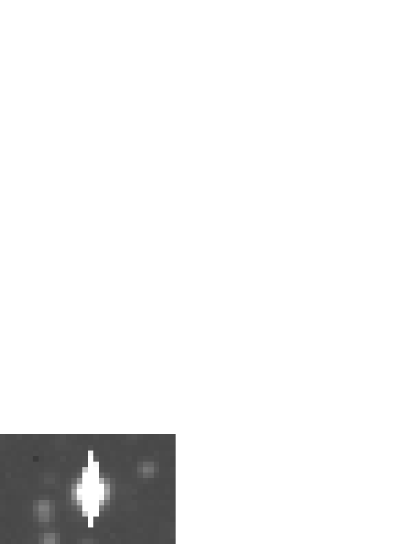
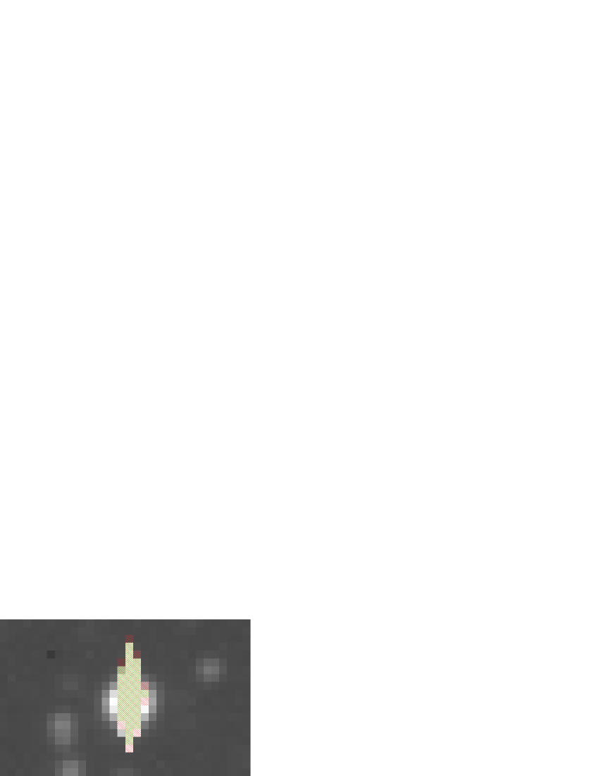
       MASKINFO= ’1 -32 16,8 -16 0,1:-2 -32 1,1 -2,1 -16 1,0:2 -1,1:3,3 -32 3,2’
MASKINFO= ’-16 -3,1:4 0,1:3,3 -32 3,0 -3,3 -16 1,0:2 0,1:-2 -32 1,0 -1,2’

Figure 2: Image stamps showing a typical saturated star and its neighborhood. The left panel shows the original image itself where the blooming structure can be seen well. The right panel shows the same area where the oversaturated and bloomed pixels are marked as follows. The oversaturated pixels (where the actual ADU values reach the maximum of the A/D converter) are marked with green right-diagonal stripes while pixels affected by blooming are marked with red left-diagonal stripes. Note that most of the oversaturated pixels are also marked as blooming ones, since their lower and/or upper neighboring pixels are also oversaturated. Such pixels are therefore marked with both red and green (left- and right-diagonal) stripes. Since the readout direction in this particular detector was vertical, the saturation/blooming structure is also vertical. The ‘‘MASKINFO’’ blocks seen below the two stamps show how this particular masking information is stored in the FITS headers in a form of special keywords.

Value	Interpretation
$T$	Use type $T$ encoding. $T=0$ implies absolute cursor movements, $T=1$ implies relative cursor movements. Other values of $T$ are reserved for optional further improvements.
$-M$	Set the current bitmask to $M$. $M$ must be between 1 and 127 and it is a bit-wise combination of the numbers 1, 2, 4, 8, 16, 32 and 64, for faulty, hot, cosmic, outer, oversaturated, blooming and interpolated pixels, respectively.
$x,y$	Move the cursor to the position $(x,y)$ (in the case of $T=0$) or shift the cursor position by $(x,y)$ (in the case of $T=1$) and mark the pixel with the mask value of $M$.
$x,y:h$	Move/shift the cursor to/by $(x,y)$ and mark the horizontal line having the length of $h$ and left endpoint at the actual position.
$x,y:-v$	Move/shift the cursor to/by $(x,y)$ and mark the vertical line having the length of $v$ and lower endpoint at the actual position.
$x,y:h,w$	Move/shift the cursor to/by $(x,y)$ and mark the rectangle having a size of $h\times w$ and lower-left corner at the actual cursor position.

Figure 3: Interpretation of the tags found MASKINFO keywords in order to decode the respective mask. The values of $M$, $h$, $v$ and $w$ must be always positive.

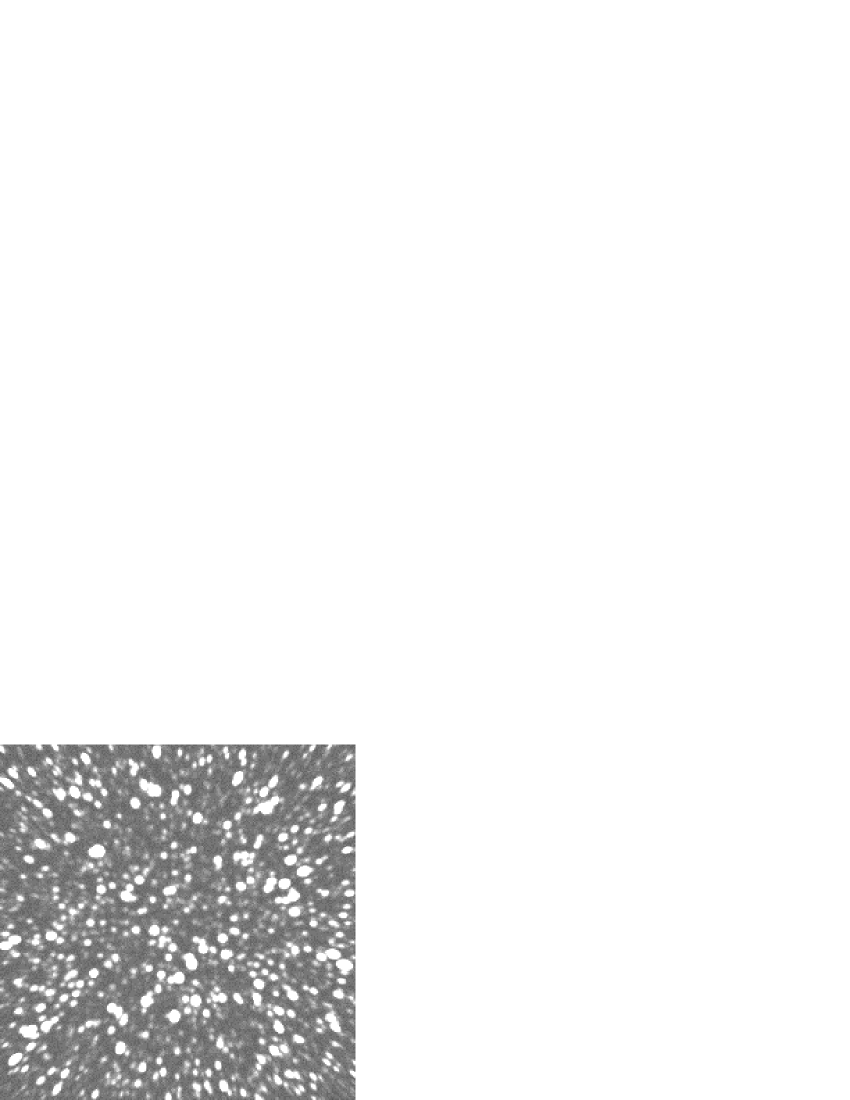
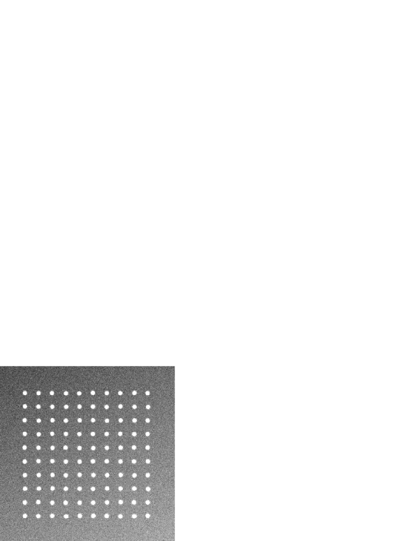
       #!/bin/sh
      
firandom --size 256,256 $\backslash$
              --list "f=3.2,500*[x=g(0,0.2),y=g(0,0.2),m=15-5*r(0,1)^2]" $\backslash$
              --list "f=3.2,1400*[x=r(-1,1),y=r(-1,1),m=15+1.38*log(r(0,1))]" $\backslash$
              --sky 100 --sky-noise 10 --integral --photon-noise --bitpix -32 --output globular.fits
      
firandom --size 256,256 $\backslash$
              --list "5000*[x=r(-1,1),y=r(-1,1),s=1.3,d=0.3*(x*x-y*y),k=0.6*x*y,m=15+1.38*log(r(0,1))]" $\backslash$
              --sky 100 --sky-noise 10 --integral --photon-noise --bitpix -32 --output coma.fits
      
firandom --size 256,256 $\backslash$
              --list "f=3.0,100*[X=36+20*div(n,10)+r(0,1),Y=36+20*mod(n,10)+r(0,1),m=10]" $\backslash$
              --sky "100+x*10-y*20" --sky-noise 10 --integral --photon-noise --bitpix -32 --output grid.fits
      
for base in globular coma grid ; do
             fiinfo ${base}.fits --pgm linear,zscale --output-pgm - | pnmtoeps -g -4 -d -o ${base}.eps
done

Figure 4: Three mock images generated using the program firandom. The first image (globular.fits) on the left shows a “globular cluster” with some field stars as well. For simplicity, the distribution of the cluster stars are Gaussian and the magnitude distribution is quadratic while the field stars distribute uniformly and their magnitudes is derived from assuming uniformly distributed stars of constant brightness. The second image (coma.fits) simulates nearly similar effect on the stellar profiles what comatic aberration would cause. The shape parameters $\delta$ and $\kappa$ (referred as d and k in the command line argument of the program) are specific functions of the spatial coordinates. The magnitude distribution of the stars is the same as for the field stars in the previous image. The third image (grid.fits) shows a set of stars positioned on a grid. The background of this image is not constant. The shell script below the image stamps is used to create these FITS files. The body of the last iterator loop in the script converts the FITS files into PGM format, using the fiinfo utility (see Sec. 3.3) and the well-known zscale intensity scaling algorithm (see DS9, Joye & Mandel, 2003). The images yielded by fiinfo are instantly converted to EPS (encapsulated Postscript) files, that is the preferred format for many typesetting systems, such as LaTeX.

3.7 Generation of artificial images – firandom

The main purpose of the program firandom is to create artificial images. These artificial images can be used either to create model images for real observations (for instance, to remove fitted stellar PSFS) or mock images that are intended to simulate some of the influence related to one or more observational artifacts and realistic effects. In principle, firandom creates an image with a given background level on which sources are drawn. Additionally, firandom is capable to add noise to the images, simulating both the effect of readout and background noise as well as photon noise. In the case of mock images, firandom is also capable to generate the object list itself. Moreover, firandom is capable to draw stellar profiles derived from PSFs (by the program fistar, see also Sec. 3.8).

The program features symbolic input processing, i.e. the variations in the background level, the spatial distribution of the object centroids (in the case of mock images), the profile shape parameters, fluxes for individual objects and the noise level can be specified not only as a tabulated dataset but in the form of arithmetic expressions. In these expressions one can involve various built-in arithmetic operators and functions, including random number generators. Of course, the generated mock coordinate lists can also be saved in tabulated form. In Fig. 4, some examples are shown that demonstrate the usage of the program firandom.

3.8 Detection of stars or point-like sources – fistar

The source detection and stellar profile modelling algorithms (see Pál, 2009b) are implemented in the program fistar. The main purpose of this program is therefore to search for and characterize point-like sources. Additionally, the program is capable to derive the point-spread function of the image, and spatial variations of the PSF can also be fitted up to arbitrary polynomial order.

The list of detected sources, their centroid coordinates, shape parameters (including FWHM) and flux estimations are written to a previously defined output file. This file can have arbitrary format, depending on our needs. The best fit PSF is saved in FITS format. If the PSF is supposed to be constant throughout the image, the FITS image is a normal two-dimensional image. Otherwise, the PSF data and the associated polynomial coefficients are stored in “data cube” format, and the size of the $z$ (NAXIS3) axis is $(N_{\rm PSF}+1)(N_{\rm PSF}+2)/2$, where $N_{\rm PSF}$ is the polynomial order used for fitting the spatial variations.

3.9 Basic coordinate list manipulations – grtrans

The main purpose of the program grtrans is to perform coordinate list transformations, mostly related to stellar profile centroid coordinates and astrometrical transformations. Since this program is used exhaustively with the program grmatch, examples and further discussion of this program can be found in the next section, Sec. 3.10.

3.10 Matching lists or catalogues – grmatch

The main purpose of the grmatch code is to implement the point matching algorithm that is the key point in the derivation of the astrometric solution and source identification. See Pál & Bakos (2006) or Pál (2009b) about more details on the algorithm itself. We note here that although the program grmatch is sufficient for point matching and source identification purposes, one may need other codes to conveniently interpret or use the output of this program. For instance, tabulated list of coordinates can be transformed from one reference frame to another, using the program grtrans while the program fitrans is capable to apply these derived transformations on FITS images, in order to, e.g. register images to the same reference frame.

       for base in ${LIST_OF_FRAMES[*]} ; do
             
             grmatch --reference $CATALOG --col-ref $COL_X,$COL_Y --col-ref-ordering -$COL_MAG $\backslash$
                          --input $AST/$base.stars --col-inp 2,3 --col-inp-ordering +8 $\backslash$
                          --weight reference,column=$COL_MAG,magnitude,power=2 $\backslash$
                          --order $AST_ORDER --max-distance $MAX_DISTANCE $\backslash$
                          --output-transformation $AST/$base.trans --output $AST/$base.match || break
                          
             grtrans $CATALOG $\backslash$
                          --col-xy $COL_X,$COL_Y --input-transformation $AST/$base.trans $\backslash$
                          --col-out $COL_X,$COL_Y --output - | $\backslash$
             grmatch --reference - --col-ref $COL_X,$COL_Y --input $AST/$base.stars --col-inp 2,3 $\backslash$
                          --match-coords --max-distance $MAX_MATCHDST --output - | $\backslash$
             grtrans --col-xy $COL_X,$COL_Y --input-transformation $AST/$base.trans --reverse $\backslash$
                          --col-out $COL_X,$COL_Y --output $AST/$base.match
             
done

Figure 5: A typical application for the grmatch – grtrans programs, for the cases where a few of the stars have high proper motion thus have significant offsets from the catalogue positions. For each frame (named $base), the input catalogue ($CATALOG) is matched with the respective list of extracted stars (found in the $AST/$base.stars file), keeping a relatively large maximum distance between the nominal and detected stellar positions ($MAX_DISTANCE, e.g. $4-6$ pixels, derived from the expected magnitude of the proper motions from the catalogue epoch and the approximate plate scale). This first initial match identifies all of the sources (including the ones with large proper motion), stored in $AST/$base.match file in the form of matched detected source and catalogue entries. However, the astrometric transformation (stored in $AST/$base.trans) is systematically affected by these high proper motion stars. In order to get rid of this effect, the match is performed again by excluding the stars with higher residual distance (by setting $MAX_MACHDIST to e.g. $1-2$ pixels). The procedure is then repeated for all frames (elements of the $LIST_OF_FRAMES[] array) in the similar manner.

3.10.1 Typical applications

As it was mentioned earlier, the programs grmatch and grtrans are generally involved in a complete photometry pipeline right after the star detection and before the instrumental photometry. If the accuracy of the coordinates in the reference catalogue is sufficient to yield a consistent plate solution, one can obtain the photometric centroids by simply invoking these programs. A more sophisticated example for these program is shown in Fig. 5. In this example these programs are invoked twice in order to both derive a proper astrometric solution and properly identify the stars with larger intrinsic proper motion. A simple direct application of grmatch and grtrans as a part of a complete photometric pipeline is displayed in Fig. 10.

3.11 Transforming and registering images – fitrans

As it is known (Pál, 2009b, Sec. 2.8), the image convolution and subtraction process requires the images to be in the same spatial reference system. The details of this registration process and the underlying algorithms have been explained in Sec. 2.7 of Pál (2009b). The purpose of the program fitrans is to implement these various image interpolation methods.

In principle, fitrans reads an image and a transformation file, performs the spatial transformation and writes the output image to a separate file. Image data are read from FITS files while the transformation files are presumably derived from the appropriate astrometric solutions. The output of the grmatch and grtrans programs can be directly passed to fitrans. Of course, fitrans takes into account the masks associated to the given image as well as derive the appropriate mask for the output file. Pixels which cannot be mapped from the original image have always a value of zero and these are marked as outer pixels (see also Sec. 3.6.1). Modern imaging systems are deployed with high-resolution detectors, therefore the spatial transformation involving exact integration on biquadratic interpolation surfaces might be a computationally expensive process (see Pál, 2009b, Sec. 2.6.3). However, distinct image transformations can be performed independently (i.e. a given transformation does not have any influence on another transformations), thus the complete registration process can easily be performed in parallel.

3.12 Convolution and image subtraction – ficonv

This member of the FITSH package is intended to implement the tasks related to the kernel fit, image convolution and subtraction. In principle, ficonv has two basic modes. First, assuming an existing kernel solution, it evaluates the basic convolution equations (Pál, 2009b, Eq. 67) on an image and writes the convolved result to a separate image file. Second, assuming a base set of kernel functions (Pál, 2009b, Eq. 73) and some model for the background variations (Pál, 2009b, Eq. 75) it derives the best fit kernel solution for the basic convolution equations. Since this fit yields a linear equation for these coefficients, the method of classic linear least squares minimization can be efficiently applied. However, the least squares matrix can have a relatively large dimension in the cases where the kernel basis is also large and/or higher order spatial variations are allowed. In the fit mode, the program yields the kernel solution, and optionally the convolved and the subtracted residual image can also be saved into separate files without additional invocations of ficonv and/or fiarith.

The program ficonv also implements the fit for cross-convolution kernels (Pál, 2009b, Eq. 79). In this case, the two kernel solutions are saved to two distinct files. Subsequent invocations of ficonv and/or fiarith can then be used to analyze various kinds of outputs.

Sec. 2.9 of Pál (2009b) discusses the relevance of the kernel solution in the case when the photometry is performed on the residual (subtracted) images. The best fit kernel solution obtained by ficonv has to be directly passed to the program fiphot (Sec. 3.13) in order to properly take into account the convolution information during the photometry (Pál, 2009b, Eq. 83).

       SELF=$0; base="$1"
if [ -n "$base" ] ; then
             fitrans ${FITS}/$base.fits $\backslash$
                          --input-transformation ${AST}/$base.trans --reverse -k -o ${REG}/$base-trans.fits
else
             pexec -f BASE.list -e base -o - -u - -c -- "$SELF $\backslash$$base"
fi

       SELF=$0; base="$1"
if [ -n "$base" ] ; then
             KERNEL="i/4;b/4;d=3/4"
             ficonv  --reference ./photref.fits $\backslash$
                          --input ${REG}/$base-trans.fits --input-stamps ./photref.reg --kernel "$KERNEL" $\backslash$
                          --output-kernel-list ${AST}/$base.kernel --output-subtracted ${REG}/$base-sub.fits
else
             pexec -f BASE.list -e base -o - -u - -c -- "$SELF $\backslash$$base"
fi

Figure 6: Two shell scripts demonstrating the invocation syntax of the fitrans and ficonv. Since the computation of the transformed and convolved images require significant amount of CPU time, the utility pexec (http://www.gnu.org/software/pexec) is used to run the jobs in parallel on multiple CPUs.

3.13 Photometry – fiphot

The program fiphot is the main code in the FITSH package that performs the raw and instrumental photometry. In the current implementation, we were focusing on the aperture photometry, performed on normal and subtracted images. Basically, fiphot reads an astronomical image (FITS file) and a centroid list file, where the latter should contain not only the centroid coordinates but the individual object identifiers as well.

In case of image subtraction-based photometry, fiphot requires also the kernel solution (derived by ficonv). Otherwise, if this information is omitted, the results of the photometry are not reliable and consistent (Pál, 2009b, Sec. 2.9).

In Fig. 10, a complete shell script is displayed, as an example of various FITSH programs related to the photometry process.

Currently, PSF photometry is not implemented directly in the program fiphot. However, the program fistar (Sec. 3.8) is capable to do PSF fitting on the detected centroids, although its output is not compatible with that of fiphot. Alternatively, lfit (see Sec. 3.16) can be used to perform profile fitting, if the pixel intensities are converted to ASCII tables in advance, however, it is not computationally efficient.

     # ${PHOT}/IMG-1.phot:
IMG-1 STAR-01 6.8765 0.0012 C
IMG-1 STAR-02 7.1245 0.0019 G
IMG-1 STAR-03 7.5645 0.0022 G
IMG-1 STAR-04 8.3381 0.0028 G
      
      
# ${PHOT}/IMG-2.phot:
IMG-2 STAR-01 6.8778 0.0012 C
IMG-2 STAR-02 7.1245 0.0020 G
IMG-2 STAR-03 7.5657 0.0023 G
IMG-2 STAR-04 8.3399 0.0029 G
      
      
# ${PHOT}/IMG-3.phot:
IMG-3 STAR-01 6.8753 0.0012 G
IMG-3 STAR-02 7.1269 0.0019 G
IMG-3 STAR-03 7.5652 0.0023 G
IMG-3 STAR-04 8.3377 0.0029 G          $\Rightarrow$          # ${LC}/STAR-01.lc:
IMG-1 STAR-01 6.8765 0.0012 C
IMG-2 STAR-01 6.8778 0.0012 C
IMG-3 STAR-01 6.8753 0.0012 G
      
# ${LC}/STAR-02.lc:
IMG-1 STAR-02 7.1245 0.0019 G
IMG-2 STAR-02 7.1245 0.0020 G
IMG-3 STAR-02 7.1269 0.0019 G
      
# ${LC}/STAR-03.lc:
IMG-1 STAR-03 7.5645 0.0022 G
IMG-2 STAR-03 7.5657 0.0023 G
IMG-3 STAR-03 7.5652 0.0023 G
      
# ${LC}/STAR-04.lc:
IMG-1 STAR-04 8.3381 0.0028 G
IMG-2 STAR-04 8.3399 0.0029 G
IMG-3 STAR-04 8.3377 0.0029 G     

       grcollect ${PHOT}/IMG-*.phot --col-base 2 --prefix ${LC}/ --extension lc --max-memory 256m
      
cat ${PHOT}/IMG-*.phot | grcollect - --col-base 2 --prefix ${LC}/ --extension lc --max-memory 256m

Figure 7: The schematics of the data transposition. Records for individual measurements are written initially to photometry files (having an extension of *.phot, for instance). These records contain the source identifiers. During the transposition, photometry files are converted to light curves. In principle, these light curves contain the same records but sorted into distinct files by the object names, not the frame identifiers. The command lines on the lower panel show some examples how this data transposition can be employed involving the program grcollect.

3.14 Transposition of tabulated data – grcollect

Raw and instrumental photometric data obtained for each frame are stored in separate files by default as it was discussed earlier (see also Sec. 3.13). We refer to these files as photometric files. In order to analyze the per-object outcome of our data reductions, one has to have the data in the form of light curve files. Therefore, the step of photometry (including the magnitude transformation) is followed immediately by the step of transposition. See Fig. 7 about how this step looks like in a simple case of 3 photometric files and 4 objects.

The main purpose of the program grcollect is to perform this transposition on the photometric data in order to have the measurements being stored in the form of light curves and therefore to be adequate for further per-object analysis (such as light curve modelling). The invocation syntax of grcollect is also shown in Fig. 7. Basically, small amount of information is needed for the transposition process: the name of the input files, the index of the column in which the object identifiers are stored and the optional prefixes and/or suffixes for the individual light curve file names. The maximum memory that the program is allowed to use is also specified in the command line argument. In fact, grcollect does not need the original data to be stored in separate files. The second example on Fig. 7 shows an alternate way of performing the transposition, namely when the whole data is read from the standard input (and the preceding command of cat dumps all the data to the standard output, these two commands are connected by a single uni-directional pipe).

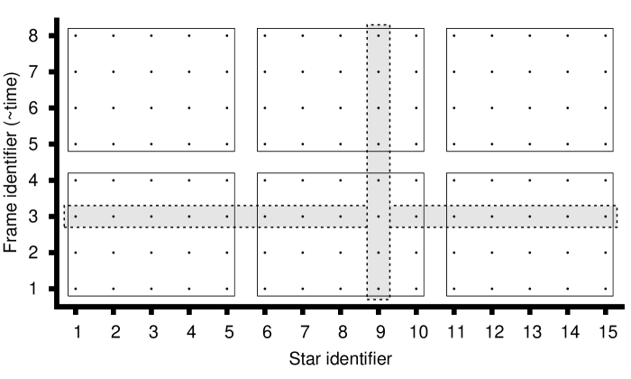
Figure 8: Storage schemes for photometric data. Supposing a series of frames, on which nearly the same set of stars have individual photometric measurements, the figure shows how these data can be arranged for practical usages. The target stars (their identifiers) are arranged along the abscissa while the ordinate shows the frame identifiers to which individual measurements (symbolized by dots) belong. Raw and instrumental photometric data are therefore represented here as rows (see the marked horizontal stripe for frame #3, for instance) while the columns refer to light curves. In practice, native ways of transposition are extremely ineffective if the total amount of data does not fit into the memory. The transposition can be speeded up by using an intermediate stage of data storage, so-called macroblocks. In the figure, each macroblock is marked by an enclosing rectangle. See text for further details.

The actual implementation of the transposition inside grcollect is very simple: it reads the data from the individual files (or from the standard input) until the data fit in the available memory. If this temporary memory is full of records, this array is sorted by the object identifier and the sorted records are written/concatenated to distinct files. The output files are named based on the appropriate object identifiers. This procedure is repeated until there are available data. Although this method creates the light curve files, it means that neither the whole process nor the access to these light curve files is effective. If either the number of the files to be transposed or the number of the records in a single file exceed a certain limit (that can be derived from the available memory, the record size and the ratio of the disk average seek time and sequential input/output bandwidth), the whole transposition process becomes highly ineffective. This can be avoided by introducing some intermediate stages of transpositions, see Fig. 8 or Pál (2009b) for further details.

Table 2: Algorithms supported by lfit and their respective requirements for the model function. The first column refers to the internal and command line identifier of the algorithms. The second column shows whether the method requires the parametric derivatives of the model functions in an analytic form or not. The third column indicates whether in the cases when the method requires parametric derivatives, should the model function be linear in all of the parameters.

Code	derivatives	linearity	Method or algorithm
L/CLLS	yes	yes	Classic linear least squares method
N/NLLM	yes	no	(Nonlinear) Levenberg-Marquardt algorithm
U/LMND	no	no	Levenberg-Marquardt algorithm employing numeric parametric derivatives
M/MCMC	no	no	Classic Markov Chain Monte-Carlo algorithm1
X/XMMC	yes	no	Extended Markov Chain Monte-Carlo2
K/MCHI	no	no	Mapping the values $\chi^{2}$ on a grid (a.k.a. “brute force” minimization)
D/DHSX	optional3	no	Downhill simplex
E/EMCE	optional4	optional4	Uncertainties estimated by refitting to synthetic data sets
A/FIMA	yes	no	Fisher Information Matrix Analysis

¹ The implemented transition function is based on the Metropolitan-Hastings algorithm and the optional Gibbs sampler. The transition amplitudes must be specified initially. Iterative MCMC can be implemented by subsequent calls of lfit, involving the previous inverse statistical variances for each parameters as the transition amplitudes for the next chain.

² The also program reports the summary related to the sanity checks (such as correlation lengths, Fisher covariance, statistical covariance, transition probabilities and the best fit value obtained by an alternate /usually the downhill simplex/ minimization).

³ The downhill simplex algorithm may use the parametric derivatives to estimate the Fisher/covariance matrix for the initial conditions in order to define the control points of the initial simplex. Otherwise, if the parametric derivatives do not exist, the user should specify the “size” of the initial simplex somehow in during the invocation of lfit.

⁴ Some of the other methods (esp. CLLS, NLLM, DHSX, in practice) can be used during the minimization process of the original data and the individual synthetic data sets.

3.15 Archiving – fizip and fiunzip

Due to the large disk space required to store the raw, calibrated and the derived (registered and/or subtracted) frames, it is essential to compress and archive the image files that are barely used. The purpose of the fizip and fiunzip programs is to compress and decompress primary FITS data, by keeping the changes in the primary FITS header to be minimal. The compressed data is stored in a one-dimensional 8 bit (BITPIX=8, NAXIS=1) array, therefore these keywords does not reflect the original image dimension or data type.

All of the other keywords are untouched. Some auxiliary information on the compression is stored in the keywords starting with “FIZIP”, the contents of these keywords depend on the involved compression method. fizip rejects compressing FITS file where such keywords exist in the primary header.

In practice, fizip and fiunzip refer to the same program (namely, fiunzip is a symbolic link to fizip) since the algorithms involved in the compression and decompression refer to the same codebase or external library. fizip and fiunzip support well known compression algorithms, such as the GNU zip (“gzip”) and the block-sorting file compressor (also known as “bzip2”) algorithm.

These compression algorithms are lossless. However, fizip supports rounding the input pixel values to the nearest integer or to the nearest fraction of some power of 2. Since the common representation of floating-point real numbers yields many zero bits if the number itself is an integer or a multiple of power of 2 (including fractional multiples), the compression is more effective if this kind of rounding is done before the compression. This “fractional rounding” yields data loss. However, if the difference between the original and the rounded values are comparable or less than the readout noise of the detector, such compression does not affect the quality of the further processing (e.g. photometry).

3.16 Generic arithmetic evaluation, regression and data analysis – lfit

Modeling of data is a prominent step in the analysis and interpretation of astronomical observations. In this section, a standalone command line driven tool, named lfit is introduced, designed for both interactive and batch processed regression analysis as well as generic arithmetic evaluation.

Similarly to the task fiarith, this tool is built on the top of the libpsn library (see Sec. 2.3). This library provides both the back-end for function evaluation as well as analytical calculations of partial derivatives. Partial derivatives are required by most of the regression methods (e.g. linear and non-linear least squares fitting) and uncertainty estimations (e.g. Fisher analysis). The program features many built-in functions related to special astrophysical problems. Moreover, it allows the end-user to extend the capabilities during run-time using dynamically loaded libraries. Sophisticated functions can be implemented and passed to lfit via this way (see e.g. Pál, 2010, for a practical case).

The built-in regression methods (Table 2), the built-in functions related to astronomical data analysis (see also Table 3) and some of the more sophisticated new tools for nonlinear regression analyses (e.g. extended Markov Chain Monte-Carlo, XMMC) are discussed in Pál (2009b) in more details.

Table 3: Basic functions found in the built-in astronomical extension library. These functions cover the fields of simple radial velocity analysis, some aspects of light curve modelling and data reduction. These functions are a kind of “common denominators”, i.e. they do not provide a direct possibility for applications but complex functions can be built on the top of them for any particular usage. All of the functions below with the exception of hjd() and bjd() have partial derivatives that can be evaluated analytically by lfit.

Function	Description
${\tt hjd}({\rm JD},\alpha,\delta)$	Function that calculates the heliocentric Julian date from the Julian day $J$ and the celestial coordinates $\alpha$ (right ascension) and $\delta$ (declination).
${\tt bjd}({\rm JD},\alpha,\delta)$	Function that calculates the barycentric Julian date from the Julian day $J$ and the celestial coordinates $\alpha$ (right ascension) and $\delta$ (declination).
${\tt ellipticK}(k)$	Complete elliptic integral of the first kind.
${\tt ellipticE}(k)$	Complete elliptic integral of the second kind.
${\tt ellipticPi}(k,n)$	Complete elliptic integral of the third kind.
${\tt eoq}(\lambda,k,h)$	Eccentric offset function, ‘q‘ component. The arguments are the mean longitude $\lambda$, in radians and the Lagrangian orbital elements $k=e\cos\varpi$, $h=e\sin\varpi$.
${\tt eop}(\lambda,k,h)$	Eccentric offset function, ‘p‘ component.
${\tt ntiu}(p,z)$	Normalized occultation flux decrease. This function calculates the flux decrease during the eclipse of two spheres when one of the spheres has uniform flux distribution and the other one by which the former is eclipsed is totally dark. The bright source is assumed to have a unity radius while the occulting disk has a radius of $p$. The distance between the centers of the two disks is $z$.
${\tt ntiq}(p,z,\gamma_{1},\gamma_{2})$	Normalized occultation flux decrease when eclipsed sphere has a non-uniform flux distribution modelled by quadratic limb darkening law. The limb darkening is characterized by $\gamma_{1}$ and $\gamma_{2}$.

       # This command just prints the content of the file ‘‘line.dat’’ to the standard output:
$ cat line.dat
2  8.10
3 10.90
4 14.05
5 16.95
6 19.90
7 23.10
# Regression: this command fits a ‘‘straight line’’ to the above data:
$ lfit -c x,y -v a,b -f ”a*x+b” -y y line.dat
     2.99714      2.01286
# Evaluation: this command evaluates the model function assuming the parameters to be known:
$ lfit -c x,y -v a=2.99714,b=2.01286 -f ”x,y,a*x+b,y-(a*x+b)” -F %6.4g,%8.2f,%8.4f,%8.4f line.dat
      2         8.10      8.0071      0.0929
      3        10.90     11.0043     -0.1042
      4        14.05     14.0014      0.0486
      5        16.95     16.9986     -0.0486
      6        19.90     19.9957     -0.0957
      7        23.10     22.9928      0.1072
$ lfit -c x,y -v a,b -f ”a*x+b” -y y line.dat –err
     2.99714      2.01286
   0.0253144     0.121842

Figure 9: These pieces of commands show the two basic operations of lfit: the first invocation of lfit fits a straight line, i.e. a model function with the form of $ax+b=y$ to the data found in the file line.dat. This file is supposed to contain two columns, one for the $x$ and one for the $y$ values. The second invocation of lfit evaluates the model function. Values for the model parameters ($a$, $b$) are taken from the command line while the individual data points ($x$, $y$) are still read from the data file line.dat. The evaluation mode allows the user to compute (and print) arbitrary functions of the model parameters and the data values. In the above example, the model function itself and the fit residuals are computed and printed, following the read values of $x$ and $y$. Note that the printed values are formatted for a minimal number significant figures (%6.4g) or for a fixed number of decimals (%8.2f or %8.4f). The last command is roughly the same as the first command for regression, but the individual uncertainties are also estimated by normalizing the value of the $\chi^{2}$ to unity.

       #!/bin/sh
CATALOG=input.cat  # name of the reference catalog
COLID=1            # column index of object identifier (in the $CATALOG file)
COLX=2             # column index of the projected X coordinate (in the $CATALOG file)
COLY=3             # column index of the projected Y coordinate (in the $CATALOG file)
COLMAG=4           # column index of object magnitude (in the $CATALOG file)
COLCOLOR=5         # column index of object color (in the $CATALOG file)
THRESHOLD=4000     # threshold for star detection
GAIN=4.2           # combined gain of the readout electronics and the A/D converter in electrons/ADU
MAGFLUX=10,10000   # magnitude/flux conversion
APERTURE=5:8:8     # aperture radius, inner radius and thickness of the background annulus (all in pixels)
mag_param=c0_00,c0_10,c0_01,c0_20,c0_11,c0_02,c1_00,c1_01,c1_10
mag_funct="c0_00+c0_10*x+c0_01*y+0.5*(c0_20*x^2+2*c0_11*x*y+c0_02*y^2)+color*(c1_00+c1_10*x+c1_01*y)"
for base in ${LIST[*]} ; do
             fistar  ${FITS}/$base.fits --algorithm uplink --prominence 0.0 --model elliptic $\backslash$
                          --flux-threshold $THRESHOLD --format id,x,y,s,d,k,amp,flux -o ${AST}/$base.stars
             grmatch --reference $CATALOG --col-ref $COLX,$COLY --col-ref-ordering -$COLMAG $\backslash$
                          --input ${AST}/$base.stars --col-inp 2,3 --col-inp-ordering +8 $\backslash$
                          --weight reference,column=$COLMAG,magnitude,power=2 $\backslash$
                          --triangulation maxinp=100,maxref=100,conformable,auto,unitarity=0.002 $\backslash$
                          --order 2 --max-distance 1 $\backslash$
                          --comment --output-transformation ${AST}/$base.trans || continue
             grtrans $CATALOG --col-xy $COLX,$COLY --col-out $COLX,$COLY $\backslash$
                          --input-transformation ${AST}/$base.trans --output - | $\backslash$
             fiphot  ${FITS}/$base.fits --input-list - --col-xy $COLX,$COLY --col-id $COLID $\backslash$
                          --gain $GAIN --mag-flux $MAGFLUX --aperture $APERTURE --disjoint-annuli $\backslash$
                          --sky-fit mode,iterations=4,sigma=3 --format IXY,MmBbS $\backslash$
                          --comment --output ${PHOT}/$base.phot
             paste   ${PHOT}/$base.phot ${PHOT}/$REF.phot $CATALOG | $\backslash$
             lfit    --columns mag:4,err:5,mag0:12,x:10,y:11,color:$((2*8+COLCOLOR)) $\backslash$
                          --variables $mag_param --function "$mag_funct" --dependent mag0-mag --error err $\backslash$
                          --output-variables ${PHOT}/$base.coeff
             paste   ${PHOT}/$base.phot ${PHOT}/$REF.phot | $\backslash$
             lfit    --columns mag:4,err:5,mag0:12,x:10,y:11,color:$((2*8+COLCOLOR)) $\backslash$
                          --variables $(cat ${PHOT}/$base.coeff) $\backslash$
                          --function "mag+($mag_funct)" --format %9.5f --column-output 4 | $\backslash$
             awk     ’{ print $1,$2,$3,$4,$5,$6,$7,$8; }’ > ${PHOT}/$base.tphot
done
for base in ${LIST[*]} ; do test -f ${PHOT}/$base.tphot && cat ${PHOT}/$base.tphot ; done | $\backslash$
grcollect - --col-base 1 --prefix $LC/ --extension .lc

Figure 10: A shell script demonstrating a complete working pipeline for time series aperture photometry. The input FITS files are read from the directory ${FITS} and their base names (without the *.fits extension) are expected to be in the array ${LIST[*]}. These base names are then used to name the files storing data obtained during the reduction process. Files created by the subsequent calls of the fistar and grmatch programs are related to the derivation of the astrometric solution and the respective files are stored in the directory ${AST}. The photometry centroids are derived from the original input catalog (found in the file $CATALOG) and the astrometric transformation (plate solution, stored in the *.trans) files. The results of the photometry are put into the directory ${PHOT}. Raw photometry is followed by the a magnitude transformation. This branch involves additional common UNIX utilities such as paste and awk in order to match the current and the reference photometry as well as to filter and resort the output after the magnitude transformation. The derivation of the transformation coefficients is done by the lfit utility, that involves $mag_funct with the parameters listed in $mag_param. This example features a quadratic magnitude transformation and a linear color dependent correction (to cancel the effects of the differential refraction). The final light curves are created by the grcollect utility what writes the individual files into the directory ${LC}. More detailed examples are available on the web page of the project, located at http://fitsh.szofi.net. These examples include further possible applications and sample data as well (that have been or are going to be published in and related to separate papers).

4 Summary

In this paper we described a software package named FITSH intended to provide a complete solution for many problems related to astronomical image processing – including calibration, source extraction, astrometry, source identification, photometry, light curve processing and regression analysis. The implementation scheme enables not only the simple and portable processing but the easy cooperation with other existing related data processing software packages. This package has an open source codebase, so any details related to the actual execution of the various tasks and algorithms can be traced. Although the current implementation allows the user a fast accomplishment of the previously listed exercises, there are some features that needs to be improved or some implementational aspects should be reconsidered. These include the cleanup of the code related to PSF analysis and some user interface functionality and homogeneity (more similar syntax for some related tasks, more sophisticated output formatting as provided by the users and so on). In order to be more compatible with existing software solutions, some improvements are considered related to the mask handling and built-in compression algorithms. In addition, implementation of features are also considered and currently in testing stage that aids the processing of data that are not related directly to “CCD imaging”. These include processing of grism observations or applications for post-processing images acquired in (near or far) infrared spectral regimes (e.g. Herschel Space Observatory). The web page of the project (http://fitsh.szofi.net) also provides a forum for the users that are open for discussions related to the FITSH package.

References

- Alard & Lupton (1998) Alard, C. & Lupton, R. H. 1998, ApJ, 503, 325
- Alard (2000) Alard, C. 2000, A&AS, 144, 363
- Bertin & Arnouts (1996) Bertin, E. & Arnouts, S. 1996, A&AS, 117, 393
- Chromey (2010) Chromey, F. R.: To Measure the Sky: An Introduction to Observational Astronomy 2010, Cambridge University Press, The Edinburgh Building, Cambridge CB2 8RU, UK
- Joye & Mandel (2003) Joye, W. A. & Mandel, E., 2003, Astronomical Data Analysis Software and Systems XII, ASP Conference Series, Vol. 295, 489 (eds. H. E. Payne, R. I. Jedrzejewski, and R. N. Hook)
- Pál & Bakos (2006) Pál, A., Bakos, G. Á., 2006, PASP, 118, 1474
- Pál (2009b) Pál, A. 2009b, PhD thesis (arXiv:0906.3486)
- Pál (2010) Pál, A., 2010, MNRAS, 409, 975
- Stetson (1987) Stetson, P. B., 1987, PASP, 99, 191
- Stetson (1989) Stetson, P. B., 1989, in Advanced School of Astrophysics, Image and Data Processing/Interstellar Dust, ed. B. Barbury, E. Janot-Pacheco, A. M. Magalhães and S. M. Viegas (São Paulo, Instituto Astrônomico e Geofísico)