On Refined Versions of the Azuma-Hoeffding Inequality with Applications in Information Theory

Abstract

This paper derives some refined versions of the Azuma-Hoeffding inequality for discrete-parameter martingales with uniformly bounded jumps, and it considers some of their potential applications in information theory and related topics. The first part of this paper derives these refined inequalities, followed by a discussion on their relations to some classical results in probability theory. It also considers a geometric interpretation of some of these inequalities, providing an insight on the inter-connections between them. The second part exemplifies the use of these refined inequalities in the context of hypothesis testing and information theory, communication, and coding theory. The paper is concluded with a discussion on some directions for further research. This work is meant to stimulate the use of some refined versions of the Azuma-Hoeffding inequality in information-theoretic aspects.

I Introduction

Inequalities providing upper bounds on probabilities of the type $\mathbb{P}(|X-\overline{x}|\geq t)$ (or $\mathbb{P}(X-\overline{x}\geq t)$ for a random variable (RV) $X$, where $\overline{x}$ denotes the expectation or median of $X$, have been among the main tools of probability theory. These inequalities are known as concentration inequalities, and they have been subject to interesting developments in probability theory. Very roughly speaking, the concentration of measure phenomenon can be stated in the following simple way: “A random variable that depends in a smooth way on many independent random variables (but not too much on any of them) is essentially constant” [62]. The exact meaning of such a statement clearly needs to be clarified rigorously, but it will often mean that such a random variable $X$ concentrates around $\overline{x}$ in a way that the probability of the event $\{|X-\overline{x}|>t\}$ decays exponentially in $t$ (for $t\geq 0$). The foundations in concentration of measures have been introduced, e.g., in [1, Chapter 7], [10, Chapter 2], [11], [36], [39], [40, Chapter 5], [41], [61] and [62]. Concentration inequalities are also at the core of probabilistic analysis of randomized algorithms (see, e.g., [1], [17], [43], [46], [54]).

The Chernoff bounds provide sharp concentration inequalities when the considered RV $X$ can be expressed as a sum of $n$ independent and bounded RVs. However, the situation is clearly more complex for non-product measures where the concentration property may not exist. Several techniques have been developed to prove concentration of measures. Among several methodologies, these concentration inequalities include isoperimetric inequalities for product measures (e.g., [61] and [62]), logarithmic-Sobolev inequalities (e.g., [27], [34] and [36, Chapter 5]), transportation-cost inequalities (e.g., [36, Chapter 6]), and the Azuma-Hoeffding inequality that is used to derive concentration inequalities for discrete-parameter martingales with bounded jumps (e.g., [1, Chapter 7], [5], [41]). The focus of this paper is on the last methodology.

The Azuma-Hoeffding inequality is by now a well-known methodology that has been often used to prove concentration phenomena. It is due to Hoeffding [30] who proved this inequality for $X=\sum_{i=1}^{n}X_{i}$ where $\{X_{i}\}$ are independent and bounded RVs, and Azuma [5] later extended it to bounded-difference martingales. Some relative entropy and exponential deviation bounds were derived in [35] for an important class of Markov chains, and these bounds are essentially identical to the Hoeffding inequality in the special case of i.i.d. RVs. A common method for proving concentration of a function $f:\mathbb{R}^{n}\rightarrow\mathbb{R}$ of $n$ independent RVs, around the expected value $\mathbb{E}[f]$, where the function $f$ is characterized by bounded differences whenever the $n$-dimensional vectors differ in only one coordinate, is called McDiarmid’s inequality (see [41, Theorem 3.1]). Some of the applications of this inequality are exemplified in [41, Section 3]. The derivation of McDiarmid’s inequality is based on introducing a martingale-difference sequence whose jumps are proved to be bounded almost surely (a.s.), and then the rest of the proof relies on the Azuma-Hoeffding inequality.

The use of the Azuma-Hoeffding inequality was introduced to the computer science literature in [58] in order to prove concentration, around the expected value, of the chromatic number for random graphs. The chromatic number of a graph is defined to be the minimal number of colors that is required to color all the vertices of this graph so that no two vertices which are connected by an edge have the same color, and the ensemble for which concentration was demonstrated in [58] was the ensemble of random graphs with $n$ vertices such that any ordered pair of vertices in the graph is connected by an edge with a fixed probability $p$ for some $p\in(0,1)$. It is noted that the concentration result in [58] was established without knowing the expected value over this ensemble. The migration of this bounding inequality into coding theory, especially for exploring some concentration phenomena that are related to the analysis of codes defined on graphs and iterative message-passing decoding algorithms, was initiated in [38], [53] and [59]. During the last decade, the Azuma-Hoeffding inequality has been extensively used for proving concentration of measures in coding theory (see, e.g., [32], [42], [45], [54] and [63]). In general, all these concentration inequalities serve to justify theoretically the ensemble approach of codes defined on graphs. However, much stronger concentration phenomena are observed in practice. The Azuma-Hoeffding inequality was also recently used in [64] for the analysis of probability estimation in the rare-events regime where it was assumed that an observed string is drawn i.i.d. from an unknown distribution, but the alphabet size and the source distribution both scale with the block length (so the empirical distribution does not converge to the true distribution as the block length tends to infinity). In another recent work [68], Azuma’s inequality was used to derive achievable rates and random coding error exponents for non-linear additive white Gaussian noise channels. This was followed by another work of the same authors [69] who used some other concentration inequalities, for discrete-parameter martingales with bounded jumps, to derive achievable rates and random coding error exponents for non-linear Volterra channels (where their bounding technique can be also applied to intersymbol-interference (ISI) channels, as was noted in [69]).

This work derives some refined versions of the Azuma-Hoeffding inequality, and it exemplifies some of their possible applications in information theory and related topics. The paper is structured as follows: Section II presents briefly some background that is essential to the analysis in this work. The core of the paper is divided into two parts. The first part includes Sections III and IV. Section III is focused on the derivation of some refined versions of Azuma’s inequality, and it considers interconnections between these bounds. Section IV considers some relations between concentration inequalities that are introduced in Section III to the method of types, central limit theorem, law of iterated logarithm, moderate deviations principle, and some previously-reported concentration inequalities for discrete-parameter martingales with bounded jumps. The second part of this work includes Sections V and VI. Section V is focused on some of the applications of these concentration inequalities to hypothesis testing and information theory, communications and coding. This paper is summarized in Section VI, followed by a discussion on some topics for further research (mainly in Shannon theory and coding). Various mathematical details of the analysis are relegated to the appendices. This work is meant to stimulate the derivation and use of some refined versions of the Azuma-Hoeffding inequality in various information-theoretic aspects.

II Preliminaries

In the following, we present briefly some background that is essential to the analysis in this work, followed by some examples that serve to motivate the continuation of this paper.

II-A Doob’s Martingales

This sub-section provides a short background on martingales to set definitions and notation. For a more thorough study of martingales, the reader it referred to standard textbooks, e.g., [8], [55] and [65].

Definition 1

[Doob’s Martingale] Let $(\Omega,\mathcal{F},\mathbb{P})$ be a probability space. A Doob’s martingale sequence is a sequence $X_{0},X_{1},\ldots$ of random variables (RVs) and corresponding sub $\sigma$-algebras $\mathcal{F}_{0},\mathcal{F}_{1},\ldots$ that satisfy the following conditions:

1. $X_{i}\in\mathbb{L}^{1}(\Omega,\mathcal{F}_{i},\mathbb{P})$ for every $i$, i.e., each $X_{i}$ is defined on the same sample space $\Omega$, it is measurable with respect to the $\sigma$-algebra $\mathcal{F}_{i}$ (i.e., $X_{i}$ is $\mathcal{F}_{i}$-measurable) and $\mathbb{E}[|X_{i}|]=\int_{\Omega}|X_{i}(\omega)|d\mathbb{P}(\omega)<\infty.$

2. $\mathcal{F}_{0}\subseteq\mathcal{F}_{1}\subseteq\ldots$ (this sequence is called a filtration).

3. For all $i\in\mathbb{N}$, $X_{i-1}=\mathbb{E}[X_{i}|\mathcal{F}_{i-1}]$ almost surely (a.s.).

In this case, it is written that $\{X_{i},\mathcal{F}_{i}\}_{i=0}^{\infty}$ or $\{X_{i},\mathcal{F}_{i}\}_{i\in\mathbb{N}_{0}}$ (with $\mathbb{N}_{0}\triangleq\mathbb{N}\cup\{0\}$) is a martingale sequence (the inclusion of $X_{\infty}$ and $\mathcal{F}_{\infty}$ in the martingale is not required here).

Remark 1

Since $\{\mathcal{F}_{i}\}_{i=0}^{\infty}$ forms a filtration, then it follows from the tower principle for conditional expectations that a.s.

$$X_{j}=\mathbb{E}[X_{i}|\mathcal{F}_{j}],\quad\forall\,i>j.$$

Also for every $i\in\mathbb{N}$, $\mathbb{E}[X_{i}]=\mathbb{E}\bigl{[}\mathbb{E}[X_{i}|\mathcal{F}_{i-1}]\bigr{]}=\mathbb{E}[X_{i-1}],$ so the expectation of a martingale sequence stays constant.

Remark 2

One can generate martingale sequences by the following procedure: Given a RV $X\in\mathbb{L}^{1}(\Omega,\mathcal{F},\mathbb{P})$ and an arbitrary filtration of sub $\sigma$-algebras $\{\mathcal{F}_{i}\}_{i=0}^{\infty}$, let

$$X_{i}=\mathbb{E}[X|\mathcal{F}_{i}],\quad\,\forall\,i\in\{0,1,\ldots\}.$$

Then, the sequence $X_{0},X_{1},\ldots$ forms a martingale since

1. The RV $X_{i}=\mathbb{E}[X|\mathcal{F}_{i}]$ is $\mathcal{F}_{i}$-measurable, and also $\mathbb{E}[|X_{i}|]\leq\mathbb{E}[|X|]<\infty$ (since conditioning reduces the expectation of the absolute value).

2. By construction $\{\mathcal{F}_{i}\}_{i=0}^{\infty}$ is a filtration.

3. For every $i\in\mathbb{N}$

   $$\mathbb{E}[X_{i}|\mathcal{F}_{i-1}]=\mathbb{E}\bigl{[}\mathbb{E}[X|\mathcal{F}_{i}]|\mathcal{F}_{i-1}\bigr{]}$$

   $$=\mathbb{E}[X|\mathcal{F}_{i-1}]\quad(\text{since}\,\mathcal{F}_{i-1}\subseteq\mathcal{F}_{i})$$

   $$=X_{i-1}\;\;\;\text{a.s.}$$

Remark 3

In continuation to Remark 2, one can choose $\mathcal{F}_{0}=\{\emptyset,\Omega\}$ and $\mathcal{F}_{n}=\mathcal{F}$, so that $X_{0},X_{1},\ldots,X_{n}$ is a martingale sequence where

$$X_{0}=\mathbb{E}[X|\mathcal{F}_{0}]=\mathbb{E}[X]\quad\text{(since $X$ is independent of $\mathcal{F}_{0}$)}$$

$$X_{n}=\mathbb{E}[X|\mathcal{F}_{n}]=X\;\;\text{a.s.}\quad\text{(since $X$ is $\mathcal{F}$-measurable)}.$$

In this case, one gets a martingale sequence where the first element is the expected value of $X$, and the last element of the sequence is $X$ itself (a.s.). This has the following interpretation: At the beginning, one doesn’t know anything about $X$, so it is initially estimated by its expectation. At each step more and more information about $X$ is revealed until one is able to specify it exactly (a.s.).

II-B Azuma’s Inequality

Azuma’s inequality forms a useful concentration inequality for bounded-difference martingales [5]. In the following, this inequality is introduced. The reader is referred to [1, Chapter 11], [10, Chapter 2], [11] and [41] for surveys on concentration inequalities for (sub/ super) martingales.

Theorem 1

[Azuma’s inequality] Let $\{X_{k},\mathcal{F}_{k}\}_{k=0}^{\infty}$ be a discrete-parameter real-valued martingale sequence such that for every $k\in\mathbb{N}$, the condition $|X_{k}-X_{k-1}|\leq d_{k}$ holds a.s. for some non-negative constants $\{d_{k}\}_{k=1}^{\infty}$. Then

$$\mathbb{P}(|X_{n}-X_{0}|\geq r)\leq 2\exp\left(-\frac{r^{2}}{2\sum_{k=1}^{n}d_{k}^{2}}\right)\,\quad\forall\,r\geq 0.$$ (1)

The concentration inequality stated in Theorem 1 was proved in [30] for independent bounded random variables, followed by a discussion on sums of dependent random variables; this inequality was later derived in [5] for bounded-difference martingales. For a proof of Theorem 1 see, e.g., [10, Chapter 2], [16, Chapter 2.4] and [43, Chapter 12]). It will be revisited in the next section for the derivation of some refined versions of Azuma’s inequality.

Remark 4

In [41, Theorem 3.13], Azuma’s inequality is stated as follows: Let $\{Y_{k},\mathcal{F}_{k}\}_{k=0}^{\infty}$ be a martingale-difference sequence with $Y_{0}=0$ (i.e., $Y_{k}$ is $\mathcal{F}_{k}$-measurable, $\mathbb{E}[|Y_{k}|]<\infty$ and $\mathbb{E}[Y_{k}|\mathcal{F}_{k-1}]=0$ a.s. for every $k\in\mathbb{N}$). Assume that, for every $k\in\mathbb{N}$, there exist numbers $a_{k},b_{k}\in\mathbb{R}$ such that a.s. $a_{k}\leq Y_{k}\leq b_{k}$. Then, for every $r\geq 0$,

$$\mathbb{P}\left(\bigg{|}\sum_{k=1}^{n}Y_{k}\bigg{|}\geq r\right)\leq 2\exp\left(-\frac{2r^{2}}{\sum_{k=1}^{n}(b_{k}-a_{k})^{2}}\right).$$ (2)

Hence, consider a discrete-parameter real-valued martingale sequence $\{X_{k},\mathcal{F}_{k}\}_{k=0}^{\infty}$ where $a_{k}\leq X_{k}-X_{k-1}\leq b_{k}$ a.s. for every $k\in\mathbb{N}$. Let $Y_{k}\triangleq X_{k}-X_{k-1}$ for every $k\in\mathbb{N}$. This implies that $\{Y_{k},\mathcal{F}_{k}\}_{k=0}^{\infty}$ is a martingale-difference sequence. From (2), it follows that for every $r\geq 0$,

$$\mathbb{P}\left(|X_{n}-X_{0}|\geq r\right)\leq 2\exp\left(-\frac{2r^{2}}{\sum_{k=1}^{n}(b_{k}-a_{k})^{2}}\right).$$ (3)

Note that according to the setting in Theorem 1, $a_{k}=-d_{k}$ and $b_{k}=d_{k}$ for every $k\in\mathbb{N}$, which implies the equivalence between (1) and (3).

As a special case of Theorem 1, let $\{X_{k},\mathcal{F}_{k}\}_{k=0}^{\infty}$ be a martingale sequence, and assume that there exists a constant $d>0$ such that a.s., for every $k\in\mathbb{N}$, $|X_{k}-X_{k-1}|\leq d.$ Then, for every $n\in\mathbb{N}$ and $\alpha\geq 0$,

$$\mathbb{P}(|X_{n}-X_{0}|\geq\alpha\sqrt{n})\leq 2\exp\left(-\frac{\alpha^{2}}{2d^{2}}\right)\,.$$ (4)

Example 1

Let $\{Y_{i}\}_{i=0}^{\infty}$ be i.i.d. binary random variables which get the values $\pm d$, for some constant $d>0$, with equal probability. Let $X_{k}=\sum_{i=0}^{k}Y_{i}$ for $k\in\{0,1,\ldots,\}$, and define the natural filtration $\mathcal{F}_{0}\subseteq\mathcal{F}_{1}\subseteq\mathcal{F}_{2}\ldots$ where

$$\mathcal{F}_{k}=\sigma(Y_{0},\ldots,Y_{k})\,,\quad\forall\,k\in\{0,1,\ldots,\}$$

is the $\sigma$-algebra that is generated by the random variables $Y_{0},\ldots,Y_{k}$. Note that $\{X_{k},\mathcal{F}_{k}\}_{k=0}^{\infty}$ is a martingale sequence, and (a.s.) $|X_{k}-X_{k-1}|=|Y_{k}|=d,\,\forall\,k\in\mathbb{N}$. It therefore follows from Azuma’s inequality in (4) that

$$\mathbb{P}(|X_{n}-X_{0}|\geq\alpha\sqrt{n})\leq 2\exp\left(-\frac{\alpha^{2}}{2d^{2}}\right).$$ (5)

for every $\alpha\geq 0$ and $n\in\mathbb{N}$. From the central limit theorem (CLT), since the RVs $\{Y_{i}\}_{i=0}^{\infty}$ are i.i.d. with zero mean and variance $d^{2}$, then $\frac{1}{\sqrt{n}}(X_{n}-X_{0})=\frac{1}{\sqrt{n}}\sum_{k=1}^{n}Y_{k}$ converges in distribution to $\mathcal{N}(0,d^{2})$. Therefore, for every $\alpha\geq 0$,

$$\lim_{n\rightarrow\infty}\mathbb{P}(|X_{n}-X_{0}|\geq\alpha\sqrt{n})=2\,Q\Bigl{(}\frac{\alpha}{d}\Bigr{)}$$ (6)

where

$$Q(x)\triangleq\frac{1}{\sqrt{2\pi}}\,\int_{x}^{\infty}\exp\Bigl{(}-\frac{t^{2}}{2}\Bigr{)}\mathrm{d}t,\quad\forall\,x\in\mathbb{R}$$ (7)

is the probability that a zero-mean and unit-variance Gaussian RV is larger than $x$. Since the following exponential upper and lower bounds on the Q-function hold

$$\frac{1}{\sqrt{2\pi}}\,\frac{x}{1+x^{2}}\cdot e^{-\frac{x^{2}}{2}}<Q(x)<\frac{1}{\sqrt{2\pi}\,x}\cdot e^{-\frac{x^{2}}{2}},\;\;\forall\,x>0$$ (8)

then it follows from (6) that the exponent on the right-hand side of (5) is the exact exponent in this example.

Example 2

In continuation to Example 1, let $\gamma\in(0,1]$, and let us generalize this example by considering the case where the i.i.d. binary RVs $\{Y_{i}\}_{i=0}^{\infty}$ have the probability law

$$\mathbb{P}(Y_{i}=+d)=\frac{\gamma}{1+\gamma},\quad\mathbb{P}(Y_{i}=-\gamma d)=\frac{1}{1+\gamma}\;.$$

Hence, it follows that the i.i.d. random variables $\{Y_{i}\}$ have zero mean and variance $\sigma^{2}=\gamma d^{2}$ as in Example 1. Let $\{X_{k},\mathcal{F}_{k}\}_{k=0}^{\infty}$ be defined similarly to Example 1, so that it forms a martingale sequence. Based on the CLT

$$\frac{X_{n}-X_{0}}{\sqrt{n}}=\frac{\sum_{k=1}^{n}Y_{k}}{\sqrt{n}}$$

weakly converges to $\mathcal{N}(0,\gamma d^{2})$, so for every $\alpha\geq 0$

$$\lim_{n\rightarrow\infty}\mathbb{P}(|X_{n}-X_{0}|\geq\alpha\sqrt{n})=2\,Q\biggl{(}\frac{\alpha}{\sqrt{\gamma}\,d}\biggr{)}.$$ (9)

From the exponential upper and lower bounds of the Q-function in (8), the right-hand side of (9) scales exponentially like $e^{-\frac{\alpha^{2}}{2\gamma d^{2}}}$. Hence, the exponent in this example is improved by a factor $\frac{1}{\gamma}$ as compared Azuma’s inequality (that is the same as in Example 1 since $|X_{k}-X_{k-1}|\leq d$ for every $k\in\mathbb{N}$). This indicates on the possible refinement of Azuma’s inequality by introducing an additional constraint on the second moment. This route was studied extensively in the probability literature, and it is further studied in Section III.

Example 2 serves to motivate the introduction of an additional constraint on the conditional variance of a martingale sequence, i.e., adding an inequality constraint of the form

$$\text{Var}(X_{k}\,|\,\mathcal{F}_{k-1})=\mathbb{E}\bigl{[}(X_{k}-X_{k-1})^{2}\,|\,\mathcal{F}_{k-1}\bigr{]}\leq\gamma d^{2}$$

where $\gamma\in(0,1]$ is a constant. Note that since, by assumption $|X_{k}-X_{k-1}|\leq d$ a.s. for every $k\in\mathbb{N}$, then the additional constraint becomes active when $\gamma<1$ (i.e., if $\gamma=1$, then this additional constraint is redundant, and it coincides with the setting of Azuma’s inequality with a fixed $d_{k}$ (i.e., $d_{k}=d$).

III Refined Versions of Azuma’s Inequality

III-A First Refinement of Azuma’s Inequality

Theorem 2

Let $\{X_{k},\mathcal{F}_{k}\}_{k=0}^{\infty}$ be a discrete-parameter real-valued martingale. Assume that, for some constants $d,\sigma>0$, the following two requirements are satisfied a.s.

$$|X_{k}-X_{k-1}|\leq d,$$

$$\text{Var}(X_{k}|\mathcal{F}_{k-1})=\mathbb{E}\bigl{[}(X_{k}-X_{k-1})^{2}\,|\,\mathcal{F}_{k-1}\bigr{]}\leq\sigma^{2}$$

for every $k\in\{1,\ldots,n\}$. Then, for every $\alpha\geq 0$,

$$\mathbb{P}(|X_{n}-X_{0}|\geq\alpha n)\leq 2\exp\left(-n\,D\biggl{(}\frac{\delta+\gamma}{1+\gamma}\Big{|}\Big{|}\frac{\gamma}{1+\gamma}\biggr{)}\right)$$ (10)

where

$$\gamma\triangleq\frac{\sigma^{2}}{d^{2}},\quad\delta\triangleq\frac{\alpha}{d}$$ (11)

and

$$D(p||q)\triangleq p\ln\Bigl{(}\frac{p}{q}\Bigr{)}+(1-p)\ln\Bigl{(}\frac{1-p}{1-q}\Bigr{)},\quad\forall\,p,q\in[0,1]$$ (12)

is the divergence (a.k.a. relative entropy or Kullback-Leibler distance) between the two probability distributions $(p,1-p)$ and $(q,1-q)$. If $\delta>1$, then the probability on the left-hand side of (10) is equal to zero.

Remark 5

Theorem 2 is known in the probability literature (see, e.g., [16, Corollary 2.4.7]), as is discussed later in Section IV-B. The reasons for introducing and proving this theorem here are as follows:

• The geometric interpretation that is associated with the proof of Theorem 2 provides an insight on the underlying connections between this theorem and some other results (e.g., Theorem 3 and Azuma’s inequality).

• The technique that is used to derive Theorem 2 serves as a starting point for the derivation of Theorem 42. Then, it is shown that under a certain sufficient condition, the exponent in Theorem 42 is better than the one in Theorem 2. This will be also exemplified numerically.

• Some of the inequalities obtained along the proof of Theorem 2 are meaningful in their own right. They serve to demonstrate, later in this work, the underlying connections of Theorem 2 with some other concentration inequalities. These inequalities are also helpful for some applications discussed in the continuation to this work.

• The proof of Theorem 2 is of interest since it indicates that it is possible to improve the exponent of inequality (10) by imposing some additional assumptions on the conditional distribution of the jumps $\xi_{k}\triangleq X_{k}-X_{k-1}$ given $\mathcal{F}_{k-1}$ (see the first item in Section VI-B).

• The inclusion of Theorem 2 and its proof at this stage makes the material self-contained, and enables the use of the same set of notation throughout the paper.

Remark 6

From the above conditions then without any loss of generality, $\sigma^{2}\leq d^{2}$ and therefore $\gamma\in(0,1]$.

Proof:

$X_{n}-X_{0}=\sum_{k=1}^{n}\xi_{k}$ where $\xi_{k}=X_{k}-X_{k-1}$ for $k=1,\ldots,n$. By assumption $|\xi_{k}|\leq d$ a.s. for some $d>0$, and also for $k=1,\ldots,n$

$$\mathbb{E}\bigl{[}\xi_{k}\,|\,\mathcal{F}_{k-1}\bigr{]}$$

$$=\mathbb{E}\bigl{[}X_{k}\,|\,\mathcal{F}_{k-1}\bigr{]}-\mathbb{E}\bigl{[}X_{k-1}\,|\,\mathcal{F}_{k-1}\bigr{]}$$

$$=\mathbb{E}\bigl{[}X_{k}\,|\,\mathcal{F}_{k-1}\bigr{]}-X_{k-1}\quad\text{(since $X_{k-1}$ is $\mathcal{F}_{k-1}$-measurable)}$$

$$=X_{k-1}-X_{k-1}=0.$$ (13)

Based on Chernoff’s inequality, it follows that for every $\alpha\geq 0$

$$\mathbb{P}(X_{n}-X_{0}\geq\alpha n)$$

$$=\mathbb{P}\left(\sum_{k=1}^{n}\xi_{k}\geq\alpha n\right)$$

$$\leq\exp(-\alpha nt)\;\mathbb{E}\biggl{[}\exp\biggl{(}t\sum_{k=1}^{n}\xi_{k}\biggr{)}\biggr{]},\quad\forall\,t\geq 0.$$ (14)

For every $t\geq 0$

$$\mathbb{E}\biggl{[}\exp\biggl{(}t\sum_{k=1}^{n}\xi_{k}\biggr{)}\biggr{]}$$

$$=\mathbb{E}\Biggl{[}\mathbb{E}\biggl{[}\exp\biggl{(}t\sum_{k=1}^{n}\xi_{k}\biggr{)}\,|\,\mathcal{F}_{n-1}\biggr{]}\Biggr{]}$$

$$=\mathbb{E}\Biggl{[}\mathbb{E}\biggl{[}\exp\biggl{(}t\sum_{k=1}^{n-1}\xi_{k}\biggr{)}\,\exp(t\xi_{n})\,|\,\mathcal{F}_{n-1}\biggr{]}\Biggr{]}$$

$$=\mathbb{E}\Biggl{[}\exp\biggl{(}t\sum_{k=1}^{n-1}\xi_{k}\biggr{)}\,\mathbb{E}\bigl{[}\exp(t\xi_{n})\,|\,\mathcal{F}_{n-1}\bigr{]}\Biggr{]}$$ (15)

where the last transition holds since $Y=\exp\bigl{(}t\sum_{k=1}^{n-1}\xi_{k}\bigr{)}$ is $\mathcal{F}_{n-1}$-measurable. The measurability of $Y$ is due to fact that $\xi_{k}\triangleq X_{k}-X_{k-1}$ is $\mathcal{F}_{k}$-measurable for every $k\in\mathbb{N}$, and $\mathcal{F}_{k}\subseteq\mathcal{F}_{n-1}$ for $0\leq k\leq n-1$ since $\{\mathcal{F}_{k}\}_{k=0}^{\infty}$ is a filtration; hence, the RV $\sum_{k=1}^{n-1}\xi_{k}$ and its exponentiation $(Y)$ are both $\mathcal{F}_{n-1}$-measurable, and a.s. $\mathbb{E}[XY|\mathcal{F}_{n-1}]=Y\,\mathbb{E}[X|\mathcal{F}_{n-1}].$

From Bennett’s inequality [7] (see, e.g., [16, Lemma 2.4.1]), if $X$ is a real-valued random variable with $\overline{x}=\mathbb{E}(X)$ and $\mathbb{E}[(X-\overline{x})^{2}]\leq\sigma^{2}$ for some $\sigma>0$, and $X\leq b$ a.s. for some $b\in\mathbb{R}$, then for every $\lambda\geq 0$

$$\mathbb{E}\bigl{[}e^{\lambda X}\bigr{]}\leq\frac{e^{\lambda\overline{x}}\left[(b-\overline{x})^{2}\exp^{-\frac{\lambda\sigma^{2}}{b-\overline{x}}}+\sigma^{2}e^{\lambda(b-\overline{x})}\right]}{(b-\overline{x})^{2}+\sigma^{2}}.$$ (16)

Applying Bennett’s inequality for the conditional law of $\xi_{k}$ given the $\sigma$-algebra $\mathcal{F}_{k-1}$, since $\mathbb{E}[\xi_{k}|\mathcal{F}_{k-1}]=0$, $\text{Var}[\xi_{k}|\mathcal{F}_{k-1}]\leq\sigma^{2}$ and $\xi_{k}\leq d$ a.s. for $k\in\mathbb{N}$, then a.s.

$$\mathbb{E}\left[\exp(t\xi_{k})\,|\,\mathcal{F}_{k-1}\right]\leq\frac{\sigma^{2}\exp(td)+d^{2}\exp\left(-\frac{t\sigma^{2}}{d}\right)}{d^{2}+\sigma^{2}}.$$ (17)

Hence, it follows from (15) and (17) that, for every $t\geq 0$,

$$\mathbb{E}\biggl{[}\exp\biggl{(}t\sum_{k=1}^{n}\xi_{k}\biggr{)}\biggr{]}$$

$$\leq\left(\frac{\sigma^{2}\exp(td)+d^{2}\exp\left(-\frac{t\sigma^{2}}{d}\right)}{d^{2}+\sigma^{2}}\right)\mathbb{E}\biggl{[}\exp\biggl{(}t\sum_{k=1}^{n-1}\xi_{k}\biggr{)}\biggr{]}$$

and, by induction, it follows that for every $t\geq 0$

$$\mathbb{E}\biggl{[}\exp\biggl{(}t\sum_{k=1}^{n}\xi_{k}\biggr{)}\biggr{]}\leq\left(\frac{\sigma^{2}\exp(td)+d^{2}\exp\left(-\frac{t\sigma^{2}}{d}\right)}{d^{2}+\sigma^{2}}\right)^{n}.$$

From the definition of $\gamma$ in (11), this inequality is rewritten as

$$\mathbb{E}\biggl{[}\exp\biggl{(}t\sum_{k=1}^{n}\xi_{k}\biggr{)}\biggr{]}\leq\left(\frac{\gamma\exp(td)+\exp(-\gamma td)}{1+\gamma}\right)^{n},\;\forall\,t\geq 0.$$ (18)

Let $x\triangleq td$ (so $x\geq 0$). Combining (14) with (18) gives that, for every $\alpha\geq 0$ (based on the definition of $\delta$ in (11), $\alpha t=\delta x$),

$$\mathbb{P}(X_{n}-X_{0}\geq\alpha n)$$

$$\leq\left(\frac{\gamma\exp\bigl{(}(1-\delta)x\bigr{)}+\exp\bigl{(}-(\gamma+\delta)x\bigr{)}}{1+\gamma}\right)^{n},\;\forall\,x\geq 0.$$ (19)

Consider first the case where $\delta=1$ (i.e., $\alpha=d$), then (19) is particularized to

$$\mathbb{P}(X_{n}-X_{0}\geq dn)\leq\left(\frac{\gamma+\exp\bigl{(}-(\gamma+1)x\bigr{)}}{1+\gamma}\right)^{n},\quad\forall\,x\geq 0$$

and the tightest bound within this form is obtained in the limit where $x\rightarrow\infty$. This provides the inequality

$$\mathbb{P}(X_{n}-X_{0}\geq dn)\leq\left(\frac{\gamma}{1+\gamma}\right)^{n}.$$ (20)

Otherwise, if $\delta\in[0,1)$, the minimization of the base of the exponent on the right-hand side of (19) w.r.t. the free non-negative parameter $x$ yields that the optimized value is

$$x=\left(\frac{1}{1+\gamma}\right)\ln\left(\frac{\gamma+\delta}{\gamma(1-\delta)}\right).$$ (21)

and its substitution into the right-hand side of (19) gives that, for every $\alpha\geq 0$,

$$\mathbb{P}(X_{n}-X_{0}\geq\alpha n)$$

$$\leq\left[\left(\frac{\gamma+\delta}{\gamma}\right)^{-\frac{\gamma+\delta}{1+\gamma}}(1-\delta)^{-\frac{1-\delta}{1+\gamma}}\right]^{n}$$

$$=\exp\left\{-n\left[\left(\frac{\gamma+\delta}{1+\gamma}\right)\ln\left(\frac{\gamma+\delta}{\gamma}\right)+\left(\frac{1-\delta}{1+\gamma}\right)\ln(1-\delta)\right]\right\}$$

$$=\exp\left(-n\,D\left(\frac{\delta+\gamma}{1+\gamma}\Big{|}\Big{|}\frac{\gamma}{1+\gamma}\right)\right)$$ (22)

and the exponent is equal to infinity if $\delta>1$ (i.e., if $\alpha>d$). Applying inequality (22) to the martingale $\{-X_{k},\mathcal{F}_{k}\}_{k=0}^{\infty}$, and using the union bound gives the two-sided concentration inequality in (10). This completes the proof of Theorem 2. ∎

Example 3

Let $d>0$ and $\varepsilon\in(0,\frac{1}{2}]$ be some constants. Consider a discrete-time real-valued martingale $\{X_{k},\mathcal{F}_{k}\}_{k=0}^{\infty}$ where a.s. $X_{0}=0$, and for every $m\in\mathbb{N}$

$$\mathbb{P}(X_{m}-X_{m-1}=d\,|\,\mathcal{F}_{m-1})=\varepsilon\,,$$

$$\mathbb{P}\left(X_{m}-X_{m-1}=-\frac{\varepsilon d}{1-\varepsilon}\,\Big{|}\,\mathcal{F}_{m-1}\right)=1-\varepsilon\,.$$

This indeed implies that a.s. for every $m\in\mathbb{N}$

$$\mathbb{E}[X_{m}-X_{m-1}\,|\,\mathcal{F}_{m-1}]=\varepsilon d+\left(-\frac{\varepsilon d}{1-\varepsilon}\right)(1-\varepsilon)=0$$

and since $X_{m-1}$ is $\mathcal{F}_{m-1}$-measurable then a.s.

$$\mathbb{E}[X_{m}\,|\,\mathcal{F}_{m-1}]=X_{m-1}.$$

Since $\varepsilon\in(0,\frac{1}{2}]$ then a.s.

$$|X_{m}-X_{m-1}|\leq\max\left\{d,\frac{\varepsilon d}{1-\varepsilon}\right\}=d.$$

From Azuma’s inequality, for every $x\geq 0$,

$$\mathbb{P}(X_{k}\geq x)\leq\exp\left(-\frac{x^{2}}{2kd^{2}}\right)$$ (23)

independently of the value of $\varepsilon$ (note that $X_{0}=0$ a.s.). The concentration inequality in Theorem 2 enables one to get a better bound: Since a.s., for every $m\in\mathbb{N}$,

$$\mathbb{E}\bigl{[}(X_{m}-X_{m-1})^{2}\,|\,\mathcal{F}_{m-1}\bigr{]}=d^{2}\varepsilon+\Bigl{(}-\frac{\varepsilon d}{1-\varepsilon}\Bigr{)}^{2}\,(1-\varepsilon)=\frac{d^{2}\varepsilon}{1-\varepsilon}$$

then from (11)

$$\gamma=\frac{\varepsilon}{1-\varepsilon}\,,\,\quad\delta=\frac{x}{d}$$

and from (22), for every $x\geq 0$,

$$\mathbb{P}(X_{k}\geq x)\leq\exp\left(-k\,D\Bigl{(}\frac{x(1-\varepsilon)}{d}+\varepsilon\;||\;\varepsilon\Bigr{)}\right).$$ (24)

Consider the case where $\varepsilon\rightarrow 0$. Then, for every $x>0$, Azuma’s inequality in (23) provides an upper bound that stays bounded away from zero, whereas the one-sided concentration inequality of Theorem 2 implies a bound in (24) that tends to zero. This exemplifies the improvement that is obtained by Theorem 2 as compared to Azuma’s inequality.

Remark 7

As was noted, e.g., in [41, Section 2], all the concentration inequalities for martingales whose derivation is based on Chernoff’s bound can be strengthened to refer to maxima. The reason is that since $\{X_{k}-X_{0},\mathcal{F}_{k}\}_{k=0}^{\infty}$ is a martingale and $h(x)=\exp(tx)$ is a monotonic increasing function for $t\geq 0$, then $\bigl{\{}\exp(t(X_{k}-X_{0})),\mathcal{F}_{k}\bigr{\}}_{k=0}^{\infty}$ is a sub-martingale for every $t\geq 0$. Hence, by applying Doob’s maximal inequality for sub-martingales, then for every $\alpha\geq 0$

$$\mathbb{P}\Bigl{(}\max_{1\leq k\leq n}X_{k}-X_{0}\geq\alpha n\Bigr{)}$$

$$=\mathbb{P}\Bigl{(}\max_{1\leq k\leq n}\exp\left(t(X_{k}-X_{0})\right)\geq\exp(\alpha nt)\Bigr{)}\quad\quad t\geq 0$$

$$\leq\exp(-\alpha nt)\;\mathbb{E}\Bigl{[}\exp\bigl{(}t(X_{n}-X_{0})\bigr{)}\Bigr{]}$$

$$=\exp(-\alpha nt)\;\mathbb{E}\left[\exp\biggl{(}t\sum_{k=1}^{n}\xi_{k}\biggr{)}\right]$$

which coincides with the proof of Theorem 2 when started from (14). This concept applies to all the concentration inequalities derived in this paper.

Corollary 1

In the setting of Theorem 2, for every $\alpha\geq 0$,

$$\mathbb{P}(|X_{n}-X_{0}|\geq\alpha n)\leq 2\exp\left(-2n\,\biggl{(}\frac{\delta}{1+\gamma}\biggr{)}^{2}\right).$$ (25)

Proof:

This concentration inequality is a loosened version of Theorem 2. From Pinsker’s inequality,

$$D(p||q)\geq\frac{V^{2}}{2},\quad\forall\,p,q\in[0,1]$$ (26)

where

$$V\triangleq||(p,1-p)-(q,1-q)||_{1}=2|p-q|$$ (27)

denotes the $L^{1}$-variational distance between the two probability distributions. Hence, for $\gamma,\delta\in[0,1]$

$$D\biggl{(}\frac{\delta+\gamma}{1+\gamma}\Big{|}\Big{|}\frac{\gamma}{1+\gamma}\biggr{)}\geq 2\left(\frac{\delta}{1+\gamma}\right)^{2}.$$

∎

Remark 8

As was shown in the proof of Corollary 25, the loosening of the exponential bound in Theorem 2 by using Pinsker’s inequality gives inequality (25). Note that (25) forms a generalization of Azuma’s inequality in Theorem 1 for the special case where, for every $i$, $d_{i}\triangleq d$ for some $d>0$. Inequality (25) is particularized to Azuma’s inequality when $\gamma=1$, and then

$$\mathbb{P}(|X_{n}-X_{0}|\geq\alpha n)\leq 2\exp\left(-\frac{n\delta^{2}}{2}\right).$$ (28)

This is consistent with the observation that if $\gamma=1$ then, from (11), the requirement in Theorem 2 for the conditional variance of the bounded-difference martingale sequence becomes redundant (since if $|X_{k}-X_{k-1}|\leq d$ a.s. then also $\mathbb{E}[(X_{k}-X_{k-1})^{2}\,|\,\mathcal{F}_{k-1}]\leq d^{2}$). Hence, if $\gamma=1$, the concentration inequality in Theorem 2 is derived under the same setting as of Azuma’s inequality.

Remark 9

The combination of the exponential bound in Theorem 2 with Pinsker’s inequality deserves further attention. Note that Pinker’s inequality is especially loose in the case where the $L^{1}$-variational distance in (27) is close to 2 (due to (27), $V\in[0,2]$ so $\frac{V^{2}}{2}$ is upper bounded by 2, whereas the divergence $D(p||q)$ can be made arbitrarily large in the limit where $V=2|p-q|$ tends to 2). Let $P$ and $Q$ be two discrete probability distributions defined on a common measurable space $(\Omega,\mathcal{F})$, and let

$$V(P,Q)\triangleq\sum_{\omega\in\Omega}|P(\omega)-Q(\omega)|$$

denote the $L^{1}$-variational distance between the probability measure $P$ and $Q$. Let

$$D\triangleq\inf_{(P,Q):V(P,Q)=V}D(P||Q)$$

be the infimum value of the information divergence subject to the constraint where the value of the $L^{1}$-variational distance is set to $V\in[0,2]$. A refinement of Pinsker’s inequality was introduced in [20, Theorem 7], and it states that

$$D\geq\frac{V^{2}}{2}+\frac{V^{4}}{36}+\frac{V^{6}}{270}+\frac{221V^{8}}{340220}.$$ (29)

However, this lower bound in (29) suffers from the same problem that it stays uniformly bounded for $V\in[0,2]$, and it is therefore especially loose for values of $V$ that are close to 2. A recent lower bound on the divergence, subject to a fixed value of the $L^{1}$-variational distance, was introduced in [25]; it states that

$$D\geq\ln\left(\frac{2}{2-V}\right)-\frac{2-V}{2}\ln\left(\frac{2+V}{2}\right)$$ (30)

which also has the pleasing property that it tends to infinity as one lets $V$ tend to 2. Note however that (30) is a looser lower bound than (29) for $V\leq 1.708$.

In the context of Theorem 2, the $L^{1}$-variational distance that corresponds to the divergence (see the exponent on the right-hand side of (10)) is equal to $V=\frac{2\delta}{1+\gamma}$. This implies that at $\gamma=1$, where $V=\delta$, then the following holds:

• Since, without any loss of generality, $\delta\triangleq\frac{\alpha}{d}$ is less than or equal to 1 (as otherwise, the right hand side of (31) due to the bounded jumps of the martingale) then the $L^{1}$-variational distance ($V$) is upper bounded by 1. Hence, according to the previous paragraph (where $V\leq 1.708$), then it follows that the lower bound in (29) gives a better lower bound on the divergence of Theorem 2 (see the right-hand side of (10)) than the lower bound in (30).

• Instead of using Pinsker’s inequality to reproduce Azuma’s inequality from Theorem 2, it is possible to apply the lower bound in (29) to get a slightly improved concentration inequality. This gives that, for every $\alpha\geq 0$,

  $$\mathbb{P}(|X_{n}-X_{0}|\geq\alpha n)$$

  $$\leq 2\exp\left[-n\left(\frac{\delta^{2}}{2}+\frac{\delta^{4}}{36}+\frac{\delta^{6}}{270}+\frac{221\delta^{8}}{340220}\right)\right].$$ (31)

  Note that, for $\delta\in[0,1]$, the exponent on the right-hand side of (31) improves the exponent of Azuma’s inequality in (28) by a marginal factor of at most 1.064 (at $\delta=1$).

Corollary 2

Let $\{X_{k},\mathcal{F}_{k}\}_{k=0}^{\infty}$ be a discrete-parameter real-valued martingale, and assume that for some constant $d>0$

$$|X_{k}-X_{k-1}|\leq d$$

a.s. for every $k\in\{1,\ldots,n\}$. Then, for every $\alpha\geq 0$,

$$\mathbb{P}(|X_{n}-X_{0}|\geq\alpha n)\leq 2\exp\left(-nf(\delta)\right)$$ (32)

where

$$f(\delta)=\left\{\begin{array}[]{ll}\ln(2)\Bigl{[}1-h_{2}\left(\frac{1-\delta}{2}\right)\Bigr{]},&0\leq\delta\leq 1\\[5.69046pt] +\infty,&\delta>1\end{array}\right.$$ (33)

and $h_{2}(x)\triangleq-x\log_{2}(x)-(1-x)\log_{2}(1-x)$ for $0\leq x\leq 1$ denotes the binary entropy function on base 2.

Proof:

By substituting $\gamma=1$ in Theorem 2 (i.e., since there is no constraint on the conditional variance, then one can take $\sigma^{2}=d^{2}$), the corresponding exponent in (10) is equal to

$$D\left(\frac{1+\delta}{2}\Big{|}\Big{|}\frac{1}{2}\right)=f(\delta)$$

since $D(p||\frac{1}{2})=\ln 2[1-h_{2}(p)]$ for every $p\in[0,1]$. ∎

Remark 10

Based on Remark 8, and since Corollary 2 is a special case of Corollary 25 when $\gamma=1$, then it follows that Corollary 2 is a tightened version of Azuma’s inequality. This can be verified directly, by comparing the exponents of (28) and (32). To this end, it is required to show that $f(\delta)>\frac{\delta^{2}}{2}$ for every $\delta>0$. If $\delta>1$, then it is obvious since $f$ is by definition infinity, whereas the right-hand side of this inequality is finite. In order to prove this inequality for $\delta\in(0,1]$, note that the power series expansion of the binary entropy function around one-half is equal to

$$h_{2}(x)=1-\frac{1}{2\ln 2}\sum_{p=1}^{\infty}\frac{(1-2x)^{2p}}{p(2p-1)},\quad 0\leq x\leq 1$$

so from (33), for every $\delta\in[0,1]$,

$$f(\delta)=\sum_{p=1}^{\infty}\frac{\delta^{2p}}{2p(2p-1)}=\frac{\delta^{2}}{2}+\frac{\delta^{4}}{12}+\frac{\delta^{6}}{30}+\frac{\delta^{8}}{56}+\frac{\delta^{10}}{90}\ldots$$ (34)

which indeed proves that $f(\delta)>\frac{\delta^{2}}{2}$ for $\delta\in(0,1]$. It is shown in Figure 1 that the two exponents in (28) and (32) nearly coincide for $\delta\leq 0.4$. Also, the improvement in the exponent of the right-hand side of (32) as compared to the exponent of Azuma’s inequality in (28) at the end point where $\delta=1$ is a by a factor $2\ln 2\approx 1.386$. This improvement in the exponent of (28) is larger than the factor of 1.064 obtained by (31). This follows from the use of the lower bound in (29) of the divergence at $\gamma=1$ in Theorem 2, instead of its exact calculation at $\gamma=1$ that leads to the improved bound in (32). As a result of this, the power series on the right-hand side of (34) replaces the exponent on the right-hand side of (31).

Discussion 1

Corollary 2 can be re-derived by the replacement of Bennett’s inequality in (17) with the inequality

$$\mathbb{E}[\exp(t\xi_{k})|\mathcal{F}_{k-1}]\leq\frac{1}{2}\bigl{[}e^{td}+e^{-td}\bigr{]}=\cosh(td)$$ (35)

that holds a.s. due to the assumption that $|\xi_{k}|\leq d$ (a.s.) for every $k$. The geometric interpretation of this inequality is based on the convexity of the exponential function, which implies that its curve is below the line segment that intersects this curve at the two endpoints of the interval $[-d,d]$. Hence,

$$\exp(t\xi_{k})\leq\frac{1}{2}\left(1+\frac{\xi_{k}}{d}\right)e^{td}+\frac{1}{2}\left(1-\frac{\xi_{k}}{d}\right)e^{-td}$$ (36)

a.s. for every $k\in\mathbb{N}$ (or vice versa since $\mathbb{N}$ is a countable set). Since, by assumption, $\{X_{k},\mathcal{F}_{k}\}_{k=0}^{\infty}$ is a martingale then $\mathbb{E}[\xi_{k}|\mathcal{F}_{k-1}]=0$ a.s. for every $k\in\mathbb{N}$, so (35) indeed follows from (36). Combined with Chernoff’s inequality, it yields (after making the substitution $x=td$ where $x\geq 0$) that

$$\mathbb{P}(X_{n}-X_{0}\geq\alpha n)\leq\bigl{(}\exp(-\delta x)\cosh(x)\bigr{)}^{n},\quad\forall\,x\geq 0.$$ (37)

This inequality leads to the derivation of Azuma’s inequality. The difference that makes Corollary 2 be a tightened version of Azuma’s inequality is that in the derivation of Azuma’s inequality, the hyperbolic cosine is replaced with the bound $\cosh(x)\leq\exp\bigl{(}\frac{x^{2}}{2}\bigr{)}$ so the inequality in (37) is loosened, and then the free parameter $x\geq 0$ is optimized to obtain Azuma’s inequality in Theorem 1 for the special case where $d_{k}\triangleq d$ for every $k\in\mathbb{N}$ (note that Azuma’s inequality handles the more general case where $d_{k}$ is not a fixed value for every $k$). In the case where $d_{k}\triangleq d$ for every $k$, Corollary 2 is obtained by an optimization of the non-negative parameter $x$ in (37). If $\delta\in[0,1]$, then by setting to zero the derivative of the logarithm of the right-hand side of (37), it follows that the optimized value is equal to $x=\tanh^{-1}(\delta)$. Substituting this value into the right-hand side of (37) provides the concentration inequality in Corollary 2; to this end, one needs to rely on the identities

$$\tanh^{-1}(\delta)=\frac{1}{2}\ln\left(\frac{1+\delta}{1-\delta}\right),\quad\cosh(x)=\bigl{(}1-\tanh^{2}(x)\bigr{)}^{-\frac{1}{2}}.$$

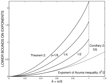
Figure 1: Plot of the lower bounds on the exponents from Azuma’s inequality in (28) and the refined inequalities in Theorem 2 and Corollary 2 (where $f$ is defined in (33)). The pointed line refers to the exponent in Corollary 2, and the three solid lines for $\gamma=\frac{1}{8},\frac{1}{4}$ and $\frac{1}{2}$ refer to the exponents in Theorem 2.

We obtain in the following a loosened version of Theorem 2.

Lemma 1

For every $x,y\in[0,1]$

$$D\left(\frac{x+y}{1+y}\Big{|}\Big{|}\frac{y}{1+y}\right)\geq\frac{x^{2}}{2y}\;B\Bigl{(}\frac{x}{y}\Bigr{)}$$ (38)

where

$$B(u)\triangleq\frac{2[(1+u)\ln(1+u)-u]}{u^{2}},\quad\forall\,u>0.$$ (39)

Proof:

This inequality follows by calculus, and it appears in [16, Exercise 2.4.21 (a)]. ∎

Corollary 3

Let $\{X_{k},\mathcal{F}_{k}\}_{k=0}^{\infty}$ be a discrete-parameter real-valued martingale that satisfies the conditions in Theorem 2. Then, for every $\alpha\geq 0$,

$$\mathbb{P}(|X_{n}-X_{0}|\geq\alpha n)$$

$$\leq 2\exp\left(-n\gamma\left[\left(1+\frac{\delta}{\gamma}\right)\ln\left(1+\frac{\delta}{\gamma}\right)-\frac{\delta}{\gamma}\right]\right)$$ (40)

where $\gamma,\delta\in[0,1]$ are introduced in (11).

Proof:

This inequality follows directly by combining inequalities (10) and (38) with the equality in (39). ∎

III-B Geometric Interpretation

The basic inequality that leads to the derivation of Azuma’s inequality (and also its tightened version in Corollary 2) relies on the convexity of the exponential function. Hence, this function is upper bounded over an arbitrary interval by the line segment that intersects the curve of this exponential function at the two endpoints of this interval. Under the additional assumption made in Theorem 2 regarding the conditional variance, one may be motivated by the above geometric viewpoint to improve Azuma’s inequality by looking for a suitable parabola that coincides with the exponential function at the two endpoints of the interval, and which forms an improved upper bound to this exponential function over the considered interval (as compared to the upper bound that is obtained by referring to the line segment that intersects the curve of the exponential function at the two endpoints of this interval, see inequality (36)). The analysis that follows from this approach leads to the following theorem.

Theorem 3

Let $\{X_{k},\mathcal{F}_{k}\}_{k=0}^{\infty}$ be a discrete-parameter real-valued martingale that satisfies the conditions in Theorem 2 with some constants $d,\sigma>0$. Then, for every $\alpha\geq 0$,

$$\mathbb{P}(|X_{n}-X_{0}|\geq\alpha n)\leq 2\exp\bigl{(}-nC(\gamma,\delta)\bigr{)}$$

where $\gamma$ and $\delta$ are introduced in (11), and the exponent in this bound is defined as follows:

• If $\delta>1$ then $C(\gamma,\delta)=\infty$.

• If $\delta=1$ then

  $$C(\gamma,\delta)=\ln\biggl{(}\frac{4}{1+\gamma}\biggr{)}.$$

• Otherwise, if $\delta\in[0,1)$, then

  $$C(\gamma,\delta)=-\ln(u+v)$$

  where

  $$u\triangleq\left(\frac{1+\gamma}{4}\right)\,e^{(1-\delta)x}$$

  $$v\triangleq\left(\frac{1}{2}+\frac{(1+2x)(1-\gamma)}{4}\right)\,e^{-(1+\delta)x}.$$

  In the above two equalities, $x\in(0,\infty)$ is given by

  $$x\triangleq-\frac{1+W_{-1}(w)}{2}-\frac{\gamma+\delta}{(1+\delta)(1-\gamma)}$$

  where $W_{-1}$ stands for a branch of the Lambert W function [12], and

  $$w\triangleq-\frac{(1+\gamma)(1-\delta)}{(1-\gamma)(1+\delta)}\cdot e^{-1-\frac{2(\gamma+\delta)}{(1+\delta)(1-\gamma)}}.$$

Proof:

See Appendix A. ∎

As is explained in the following discussion, Theorem 3 is looser than Theorem 2 (though it improves Corollary 2 and Azuma’s inequality that are independent of $\gamma$). The reason for introducing Theorem 3 here is in order to emphasize the geometric interpretation of the concentration inequalities that were introduced so far, as is discussed in the following.

Discussion 2

A common ingredient in proving Azuma’s inequality, and Theorems 2 and 3 is a derivation of an upper bound on the conditional expectation $\mathbb{E}\bigl{[}e^{t\xi_{k}}\,|\,\mathcal{F}_{k-1}\bigr{]}$ for $t\geq 0$ where $\mathbb{E}\bigl{[}\xi_{k}\,|\,\mathcal{F}_{k-1}\bigr{]}=0$, $\text{Var}\bigl{[}\xi_{k}|\mathcal{F}_{k-1}\bigr{]}\leq\sigma^{2}$, and $|\xi_{k}|\leq d$ a.s. for some $\sigma,d>0$ and for every $k\in\mathbb{N}$. The derivation of Azuma’s inequality and Corollary 2 is based on the line segment that connects the curve of the exponent $y(x)=e^{tx}$ at the endpoints of the interval $[-d,d]$; due to the convexity of $y$, this chord is above the curve of the exponential function $y$ over the interval $[-d,d]$. The derivation of Theorem 2 is based on Bennett’s inequality which is applied to the conditional expectation above. The proof of Bennett’s inequality (see, e.g., [16, Lemma 2.4.1]) is shortly reviewed, while adopting its proof to our notation, for the continuation of this discussion. Let $X$ be a random variable with zero mean and variance $E[X^{2}]=\sigma^{2}$, and assume that $X\leq d$ a.s. for some $d>0$. Let $\gamma\triangleq\frac{\sigma^{2}}{d^{2}}$. The geometric viewpoint of Bennett’s inequality is based on the derivation of an upper bound on the exponential function $y$ over the interval $(-\infty,d]$; this upper bound on $y$ is a parabola that intersects $y$ at the right endpoint $(d,e^{td})$ and is tangent to the curve of $y$ at the point $(-\gamma d,e^{-t\gamma d})$. As is verified in the proof of [16, Lemma 2.4.1], it leads to the inequality $y(x)\leq\varphi(x)$ for every $x\in(-\infty,d]$ where $\varphi$ is the parabola that satisfies the conditions

$$\varphi(d)=y(d)=e^{td},$$

$$\varphi(-\gamma d)=y(-\gamma d)=e^{-t\gamma d},$$

$$\varphi^{\prime}(-\gamma d)=y^{\prime}(-\gamma d)=te^{-t\gamma d}.$$

Calculation shows that this parabola admits the form

$$\varphi(x)=\frac{(x+\gamma d)e^{td}+(d-x)e^{-t\gamma d}}{(1+\gamma)d}+\frac{\alpha[\gamma d^{2}+(1-\gamma)d\;x-x^{2}]}{(1+\gamma)^{2}d^{2}}$$

where $\alpha\triangleq\bigl{[}(1+\gamma)td+1\bigr{]}e^{-t\gamma d}-e^{td}$. At this point, since $\mathbb{E}[X]=0$, $\mathbb{E}[X^{2}]=\gamma d^{2}$ and $X\leq d$ a.s., then the following bound holds:

$$\mathbb{E}\bigl{[}e^{tX}\bigr{]}\leq\mathbb{E}\bigl{[}\varphi(X)\bigr{]}$$

$$=\frac{\gamma e^{td}+e^{-\gamma td}}{1+\gamma}+\alpha\left(\frac{\gamma d^{2}-\mathbb{E}[X^{2}]}{(1+\gamma)^{2}d^{2}}\right)$$

$$=\frac{\gamma e^{td}+e^{-\gamma td}}{1+\gamma}$$

$$=\frac{\mathbb{E}[X^{2}]e^{td}+d^{2}e^{-\frac{t\mathbb{E}[X^{2}]}{d}}}{d^{2}+\mathbb{E}[X^{2}]}$$

which indeed proves Bennett’s inequality in the considered setting, and it also provides a geometric viewpoint to the proof of this inequality. Note that under the above assumption, the bound is achieved with equality when $X$ is a RV that gets the two values $+d$ and $-\gamma d$ with probabilities $\frac{\gamma}{1+\gamma}$ and $\frac{1}{1+\gamma}$, respectively. This bound also holds when $\mathbb{E}[X^{2}]\leq\sigma^{2}$ since the right-hand side of the inequality is a monotonic non-decreasing function of $\mathbb{E}[X^{2}]$ (as it was verified in the proof of [16, Lemma 2.4.1]).

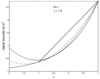
Figure 2: The function $y=e^{x}$ (solid line), and the upper bounds on this function that are used to derive Azuma’s inequality and Corollary 2 (the dashed line segment intersecting the exponential function at the endpoints of the interval $[-d,d]$), Theorem 2 (the pointed line for the parabola that coincides with the exponential function at $x=d$ and is tangent to this function at $x=-\gamma d$), and Theorem 3 (the dash-dot line for the parabola that coincides with the exponential function at $x=d$ and is tangent to this function at $x=-d$). These parabolas are upper bounds on the exponential function over $(-\infty,d]$.

Applying Bennett’s inequality to the conditional law of $\xi_{k}$ given $\mathcal{F}_{k-1}$ gives (17) (with $\gamma$ in (11)). From this discussion, the parabola that serves for the derivation of Bennett’s inequality is the best one in the sense that it achieves the minimal upper bound on the conditional expectation $\mathbb{E}\bigl{[}e^{t\xi_{k}}\,|\,\mathcal{F}_{k-1}\bigr{]}$ (where $t\geq 0$) with equality for a certain conditional probability distribution. In light of this geometric interpretation, it follows from the proof of Theorem 3 that the concentration inequality in this theorem is looser than the one in Theorem 2. The reason is that the underlying parabola that serves to get an upper bound on the exponential function in Theorem 3 is the parabola that intersects $y$ at $x=d$ and is tangent to the curve of this exponent at $x=-d$; as is illustrated in Figure 2, this parabola forms an upper bound on the exponential function $y$ over the interval $(-\infty,d]$. On the other hand, Theorem 3 refines Azuma’s inequality and Corollary 2 since the chord that connects the curve of the exponential function at the two endpoints of the interval $[-d,d]$ is replaced by a tighter upper bound which is the parabola that coincides with the exponent at the two endpoints of this interval. Figure 2 compares the three considered upper bounds on the exponential function that serve for the derivation of Azuma’s inequality (and Corollary 2), and Theorems 2 and 3. A comparison of the resulting bounds on the exponents of these inequalities and some other bounds that are derived later in this section is shown in Figure 3; it verifies that indeed the exponent of Theorem 2 is superior over the exponent in Theorem 3, but this difference is reduced by increasing the value of $\gamma\in(0,1]$ (e.g., for $\gamma=\frac{3}{4}$, this difference is already marginal). The reason for this observation is that the two underlying parabolas that serve for the derivation of Theorems 2 and 3 almost coincide when the value of $\gamma$ is approached to 1 (and they are exactly the same parabola when $\gamma=1$); in this respect, note that the left tangent point at $x=-\gamma d$ for the parabola that refers to the derivation of Theorem 2 (via Bennet’s inequality) tends to the left endpoint of the interval $[-d,d]$ as $\gamma\rightarrow 1$, and therefore the two parabolas almost coincide for $\gamma$ close to 1.

III-C Another Approach for the Derivation of a Refinement of Azuma’s Inequality

Theorem 4

Let $\{X_{k},\mathcal{F}_{k}\}_{k=0}^{\infty}$ be a discrete-parameter real-valued martingale, and let $m\in\mathbb{N}$ be an even number. Assume that the following conditions hold a.s. for every $k\in\mathbb{N}$

$$|X_{k}-X_{k-1}|\leq d,$$

$$\Big{|}\mathbb{E}\bigl{[}(X_{k}-X_{k-1})^{l}\,|\,\mathcal{F}_{k-1}\bigr{]}\Big{|}\leq\mu_{l},\quad l=2,\ldots,m$$

for some $d>0$ and non-negative numbers $\{\mu_{l}\}_{l=2}^{m}$. Then, for every $\alpha\geq 0$,

$$\mathbb{P}(|X_{n}-X_{0}|\geq n\alpha)$$

$$\leq 2\left\{\inf_{x\geq 0}\,e^{-\delta x}\left[1+\sum_{l=2}^{m-1}\frac{(\gamma_{l}-\gamma_{m})x^{l}}{l!}+\gamma_{m}(e^{x}-1-x)\right]\right\}^{n}$$

(41)

where

$$\delta\triangleq\frac{\alpha}{d},\quad\gamma_{l}\triangleq\frac{\mu_{l}}{d^{l}},\;\;\forall\;l=2,\ldots,m.$$ (42)

Proof:

The starting point of this proof relies on (14) and (15) that were used for the derivation of Theorem 2. From this point, we deviate from the proof of Theorem 2. For every $k\in\mathbb{N}$ and $t\geq 0$

$$\mathbb{E}\bigl{[}\exp(t\xi_{k})|\mathcal{F}_{k-1}\bigr{]}$$

$$=1+t\mathbb{E}\bigl{[}\xi_{k}|\mathcal{F}_{k-1}\bigr{]}+\ldots+\frac{t^{m-1}}{(m-1)!}\cdot\mathbb{E}\bigl{[}(\xi_{k})^{m-1}|\mathcal{F}_{k-1}\bigr{]}$$

$$+\mathbb{E}\left[\exp(t\xi_{k})-1-t\xi_{k}-\ldots-\frac{t^{m-1}(\xi_{k})^{m-1}}{(m-1)!}\right]$$

$$=1+t\mathbb{E}\bigl{[}\xi_{k}|\mathcal{F}_{k-1}\bigr{]}+\ldots+\frac{t^{m-1}}{(m-1)!}\cdot\mathbb{E}\bigl{[}(\xi_{k})^{m-1}|\mathcal{F}_{k-1}\bigr{]}$$

$$+\frac{t^{m}}{m!}\cdot\mathbb{E}\bigl{[}(\xi_{k})^{m}\varphi_{m}(t\xi_{k})|\mathcal{F}_{k-1}\bigr{]}$$ (43)

where

$$\varphi_{m}(y)\triangleq\left\{\begin{array}[]{ll}\frac{m!}{y^{m}}\left(e^{y}-\sum_{l=0}^{m-1}\frac{y^{l}}{l!}\right)&\mbox{if}\;y\neq 0\\ 1&\mbox{if}\;y=0\end{array}\right..$$ (44)

In order to proceed, we need the following lemma:

Lemma 2

Let $m\in\mathbb{N}$ be an even number, then the function $\varphi_{m}$ has the following properties:

1. $\lim_{y\rightarrow 0}\varphi_{m}(y)=1$, so $\varphi_{m}$ is a continuous function.

2. $\varphi_{m}$ is monotonic increasing over the interval $[0,\infty)$.

3. $0<\varphi_{m}(y)<1$ for every $y<0$.

4. $\varphi_{m}$ is a non-negative function.

Proof:

See Appendix B. ∎

Remark 11

Note that [23, Lemma 3.1] states that $\varphi_{2}$ is a monotonic increasing and non-negative function over the real line. In general, for an even $m\in\mathbb{N}$, the properties of $\varphi_{m}$ in Lemma 2 are sufficient for the continuation of the proof.

From (43) and Lemma 2, since $\xi_{k}\leq d$ a.s. and $m$ is even, then it follows that for an arbitrary $t\geq 0$

$$\varphi_{m}(t\xi_{k})\leq\varphi_{m}(td),\quad\forall\,k\in\mathbb{N}$$ (45)

a.s. (to see this, lets separate the two cases where $\xi_{k}$ is either non-negative or negative. If $0\leq\xi_{k}\leq d$ a.s. then, for $t\geq 0$, inequality (45) holds (a.s.) due to the monotonicity of $\varphi_{m}$ over $[0,\infty)$. If $\xi_{k}<0$ then the second and third properties in Lemma 2 yield that, for $t\geq 0$ and every $k\in\mathbb{N}$,

$$\varphi_{m}(t\xi_{k})\leq 1=\varphi_{m}(0)\leq\varphi_{m}(td),$$

so in both cases inequality (45) is satisfied a.s.). Since $m$ is even then $(\xi_{k})^{m}\geq 0$, and

$$\mathbb{E}\bigl{[}(\xi_{k})^{m}\,\varphi_{m}(t\xi_{k})|\mathcal{F}_{k-1}\bigr{]}\leq\varphi_{m}(td)\,\mathbb{E}\bigl{[}(\xi_{k})^{m}|\mathcal{F}_{k-1}\bigr{]},\;\;\forall\,t\geq 0.$$

Also, since $\{X_{k},\mathcal{F}_{k}\}_{k=0}^{\infty}$ is a martingale then $\mathbb{E}\bigl{[}\xi_{k}|\mathcal{F}_{k-1}\bigr{]}=0,$ and based on the assumptions of this theorem

$$\mathbb{E}[(\xi_{k})^{l}|\mathcal{F}_{k-1}]\leq\mu_{l}=d^{l}\gamma_{l},\quad\forall\,l\in\{2,\dots,m\}.$$

By substituting the last three results on the right-hand side of (43), it follows that for every $t\geq 0$ and every $k\in\mathbb{N}$

$$\mathbb{E}\bigl{[}\exp(t\xi_{k})|\mathcal{F}_{k-1}\bigr{]}\leq 1+\sum_{l=2}^{m-1}\frac{\gamma_{l}\,(td)^{l}}{l!}+\frac{\gamma_{m}\,(td)^{m}\,\varphi_{m}(td)}{m!}$$ (46)

so from (15)

$$\mathbb{E}\left[\exp\Bigl{(}t\sum_{k=1}^{n}\xi_{k}\Bigr{)}\right]$$

$$\leq\left(1+\sum_{l=2}^{m-1}\frac{\gamma_{l}\,(td)^{l}}{l!}+\frac{\gamma_{m}\,(td)^{m}\,\varphi_{m}(td)}{m!}\right)^{n},\;\;\forall\,t\geq 0.$$ (47)

From (14), if $\alpha\geq 0$ is arbitrary, then for every $t\geq 0$

$$\mathbb{P}(X_{n}-X_{0}\geq\alpha n)$$

$$\leq\exp(-\alpha nt)\left(1+\sum_{l=2}^{m-1}\frac{\gamma_{l}\,(td)^{l}}{l!}+\frac{\gamma_{m}\,(td)^{m}\,\varphi_{m}(td)}{m!}\right)^{n}\;.$$

Let $x\triangleq td$. Then, based on (11) and (44), for every $\alpha\geq 0$

$$\mathbb{P}(X_{n}-X_{0}\geq\alpha n)$$

$$\leq\left\{\inf_{x\geq 0}e^{-\delta x}\left(1+\sum_{l=2}^{m-1}\frac{\gamma_{l}\,x^{l}}{l!}+\frac{\gamma_{m}x^{m}\,\varphi_{m}(x)}{m!}\right)\right\}^{n}$$

$$=\left\{\inf_{x\geq 0}e^{-\delta x}\left[1+\sum_{l=2}^{m-1}\frac{\gamma_{l}\,x^{l}}{l!}+\gamma_{m}\left(e^{x}-\sum_{l=0}^{m-1}\frac{x^{l}}{l!}\right)\right]\right\}^{n}$$

$$=\left\{\inf_{x\geq 0}e^{-\delta x}\left[1+\sum_{l=2}^{m-1}\frac{(\gamma_{l}-\gamma_{m})\,x^{l}}{l!}+\gamma_{m}\left(e^{x}-1-x\right)\right]\right\}^{n}.$$

(48)

The two-sided concentration inequality in (41) follows by applying the above one-sided inequality to the martingale $\{-X_{k},\mathcal{F}_{k}\}_{k=0}^{\infty}$, and using the union bound. ∎

Remark 12

Without any loss of generality, it is assumed that $\alpha\in[0,d]$ (as otherwise, the considered probability is zero for $\alpha>d$). Based on the above conditions, it is also assumed that $\mu_{l}\leq d^{l}$ for every $l\in\{2,\ldots,m\}$. Hence, $\delta\in[0,1]$, and $\gamma_{l}\in[0,1]$ for all values of $l$. Note that, from (11), $\gamma_{2}=\gamma$.

Remark 13

From the proof of Theorem 42, it follows that the one-sided inequality (48) is satisfied if the martingale $\{X_{k},\mathcal{F}_{k}\}_{k=0}^{n}$ fulfills the following conditions a.s.

$$X_{k}-X_{k-1}\leq d,$$

$$\mathbb{E}\bigl{[}(X_{k}-X_{k-1})^{l}\,|\,\mathcal{F}_{k-1}\bigr{]}\leq\mu_{l},\quad l=2,\ldots,m$$

for some $d>0$ and non-negative numbers $\{\mu_{l}\}_{l=2}^{m}$. Note that these conditions are weaker than those that are stated in Theorem 42. Under these weaker conditions, $\gamma_{l}\triangleq\frac{\mu_{l}}{d^{l}}$ may be larger than 1. This remark will be helpful later in this paper.

III-C1 Specialization of Theorem 42 for $m=2$

Theorem 42 with $m=2$ (i.e., when the same conditions as of Theorem 2 hold) is expressible in closed form, as follows:

Corollary 4

Let $\{X_{k},\mathcal{F}_{k}\}_{k=0}^{\infty}$ be a discrete-parameter real-valued martingale that satisfies a.s. the conditions in Theorem 2. Then, for every $\alpha\geq 0$,

$$\mathbb{P}(|X_{n}-X_{0}|\geq\alpha n)\leq 2\exp\bigl{(}-nC(\gamma,\delta)\bigr{)}$$

where $\gamma$ and $\delta$ are introduced in (11), and the exponent in this upper bound gets the following form:

• If $\delta>1$ then $C(\gamma,\delta)=\infty$.

• If $\delta=1$ then

  $$C(\gamma,\delta)=\frac{1}{\gamma}-\ln\Bigl{(}\gamma\bigl{(}e^{\frac{1}{\gamma}}-1\bigr{)}\Bigr{)}.$$

• Otherwise, if $\delta\in(0,1)$, then

  $$C(\gamma,\delta)=\delta x-\ln\bigl{(}1+\gamma(e^{x}-1-x)\bigr{)}$$

  where $x\in\bigl{(}0,\frac{1}{\gamma}\bigr{)}$ is given by

  $$x=\frac{1}{\gamma}+\frac{1}{\delta}-1-W_{0}\left(\frac{(1-\delta)e^{\frac{1}{\gamma}+\frac{1}{\delta}-1}}{\delta}\right)$$ (49)

  and $W_{0}$ denotes the principal branch of the Lambert W function [12].

Proof:

See Appendix C. ∎

Proposition 1

If $\gamma<\frac{1}{2}$ then Corollary 4 gives a stronger result than Corollary 2 (and, hence, it is also better than Azuma’s inequality).

Proof:

See Appendix D. ∎

It is of interest to compare the tightness of Theorem 2 and Corollary 4. This leads to the following conclusion:

Proposition 2

The concentration inequality in Corollary 4 is looser than Theorem 2.

Proof:

See Appendix E. ∎

The statements in Propositions 1 and 2 are illustrated in Figure 3. Sub-plots (a) and (b) in Figure 3 refer to $\gamma\leq\frac{1}{2}$ where the statement in Proposition 1 holds. On the other hand, sub-plots (c) and (d) in Figure 3 refer to higher values of $\gamma$, and therefore the statement in Proposition 1 does not apply to these values of $\gamma$.

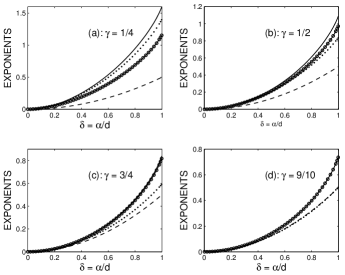
Figure 3: Plots of the exponents $c\triangleq c(\gamma,\delta)$ for bounds of the form $\mathbb{P}\{|X_{n}-X_{0}|\geq n\alpha\}\leq e^{-nc(\gamma,\delta)}$ for an arbitrary $\alpha\geq 0$. The sequence $\{X_{k},\mathcal{F}_{k}\}_{k=0}^{\infty}$ is a discrete-parameter martingale that satisfies the conditions in Theorem 2 for some positive constants $d$ and $\sigma$ (without loss of generality, $\sigma\leq d$), and where $\gamma\in(0,1]$ and $\delta\in[0,1]$ are introduced in (11). The plots show lower bounds on the exponents according to Azuma’s inequality in (28), the bounds in Theorems 2 and 3 Corollary 4. The plots are depicted for a fixed value of $\gamma\triangleq\frac{\sigma^{2}}{d^{2}}$; the horizontal axes refer to the parameter $\delta\triangleq\frac{\alpha}{d}$, and the vertical axes refer to the lower bounds on the exponents $c(\gamma,\delta)$. The dashed lines refer to Azuma’s inequality, the solid lines refer to Theorem 2, the circled lines refer to Theorem 3, and the pointed lines refer to Corollary 4. The subplots (a)-(d) correspond to values of $\gamma=\frac{1}{4},\frac{1}{2},\frac{3}{4}$ and $\frac{9}{10}$, respectively.

III-C2 Exploring the Dependence of the Bound in Theorem 42 in Terms of $m$

In the previous sub-section, a closed-form expression of Theorem 42 was obtained for the special case where $m=2$ (see Corollary 4), but also Proposition 2 demonstrated that this special case is looser than Theorem 2 (which is also given as a closed-form expression). Hence, it is natural to enquire how does the bound in Theorem 42 vary in terms of $m$ (where $m\geq 2$ is even), and if there is any chance to improve Theorem 2 for larger values of $m$. Also, in light of the closed-form expression that was given in Corollary 4 for the special case where $m=2$, it would be also pleasing to get an inequality that is expressed in closed form for a general even number $m\geq 2$. The continuation of the study in this sub-section is outlined as follows:

• A loosened version of Theorem 42 is introduced, and it is shown to provide an inequality whose tightness consistently improves by increasing the value of $m$. For $m=2$, this loosened version coincides with Theorem 42. Hence, it follows (by introducing this loosened version) that $m=2$ provides the weakest bound in Theorem 42.

• Inspired by the closed-form expression of the bound in Corollary 4, we derive a closed-form inequality (i.e., a bound that is not subject to numerical optimization) by either loosening Theorem 42 or further loosening its looser version from the previous item. As will be exemplified numerically in Section V, the closed-form expression of the new bound causes to a marginal loosening of Theorem 42. Also, for $m=2$, it is exactly Theorem 42.

• A necessary and sufficient condition is derived for the case where, for an even $m\geq 4$, Theorem 42 provides a bound that is exponentially advantageous over Theorem 2. Note however that, when $m\geq 4$ in Theorem 42, one needs to calculate conditional moments of the martingale differences that are of higher orders than 2; hence, an improvement in Theorem 42 is obtained at the expense of the need to calculate higher-order conditional moments. Saying this, note that the derivation of Theorem 42 deviates from the proof of Theorem 2 at an early stage, and it cannot be considered as a generalization of Theorem 2 when higher-order moments are available (as is also evidenced in Proposition 2 which demonstrates that, for $m=2$, Theorem 42 is weaker than Theorem 2).

• Finally, this sufficient condition is particularized in the asymptotic case where $m\rightarrow\infty$. It is of interest since the tightness of the loosened version of Theorem 42 from the first item is improved by increasing the value of $m$.

The analysis that is related to the above outline is presented in the following. Then, following this analysis, numerical results that are related to the comparison of Theorems 2 and 42 are relegated to Section V (while considered in a certain communication-theoretic context).

Corollary 5

Let $\{X_{k},\mathcal{F}_{k}\}_{k=0}^{n}$ be a discrete-parameter real-valued martingale, and let $m\in\mathbb{N}$ be an even number. Assume that $|X_{k}-X_{k-1}|\leq d$ holds a.s. for every $k\in\mathbb{N}$, and that there exists a (non-negative) sequence $\{\mu_{l}\}_{l=2}^{m}$ so that for every $k\in\mathbb{N}$

$$\mu_{l}=\mathbb{E}[|X_{k}-X_{k-1}|^{l}\,|\,\mathcal{F}_{k-1}],\quad\forall\,l=2,\ldots,m.$$ (50)

Then, inequality (41) holds with the notation in (42).

Proof:

This corollary is a consequence of Theorem 42 since

$$|\mathbb{E}[(X_{k}-X_{k-1})^{l}\,|\,\mathcal{F}_{k-1}]|\leq\mathbb{E}[|X_{k}-X_{k-1}|^{l}\,|\,\mathcal{F}_{k-1}].$$

∎

Proposition 3

Theorem 42 and Corollary 5 coincide for $m=2$ (hence, Corollary 5 provides in this case the result stated in Corollary 4). Furthermore, the bound in Corollary 5 improves as the even value of $m\in\mathbb{N}$ is increased.

Proof:

See Appendix F. ∎

Inspired by the closed-form inequality that follows from Theorem 42 for $m=2$ (see Corollary 4), a closed-form inequality is suggested in the following by either loosening Theorem 42 or Corollary 5. It generalizes the result in Corollary 4, and it coincides with Theorem 42 and Corollary 5 for $m=2$.

Corollary 6

Under the conditions of Corollary 5 then, for every $\alpha\geq 0$,

$$\mathbb{P}(X_{n}-X_{0}\geq n\alpha)$$

$$\leq\,\left\{e^{-\delta x}\left[1+\sum_{l=2}^{m-1}\frac{(\gamma_{l}-\gamma_{m})x^{l}}{l!}+\gamma_{m}(e^{x}-1-x)\right]\right\}^{n}$$

(51)

where $\{\gamma_{l}\}_{l=2}^{m}$ and $\delta$ are introduced in (42),

$$x=\frac{a+b}{c}-W_{0}\left(\frac{b}{c}\cdot e^{\frac{a+b}{c}}\right)$$ (52)

with $W_{0}$ that denotes the principal branch of the Lambert W function [12], and

$$a\triangleq\frac{1}{\gamma_{2}},\quad b\triangleq\frac{\gamma_{m}}{\gamma_{2}}\left(\frac{1}{\delta}-1\right),\quad c\triangleq\frac{1}{\delta}-b.$$ (53)

Proof:

See Appendix G. ∎

Remark 14

It is exemplified numerically in Section V that the replacement of the infimum over $x\geq 0$ on the right-hand side of (41) with the sub-optimal choice of the value of $x$ that is given in (52) and (53) implies a marginal loosening in the exponent of the bound. Note also that, for $m=2$, this value of $x$ is optimal since it coincides with the exact value in (49).

Corollary 7

Under the assumptions of Theorem 2 then, for every $\alpha\geq 0$,

$$\mathbb{P}(X_{n}-X_{0}\geq n\alpha)\leq e^{-nE}$$ (54)

where

$$E=E_{2}(\gamma_{2},\delta)\triangleq D\left(\frac{\delta+\gamma_{2}}{1+\gamma_{2}}\Big{|}\Big{|}\frac{\gamma_{2}}{1+\gamma_{2}}\right).$$ (55)

Also, under the assumptions of Theorem 42 or Corollary 5 then (54) holds for every $\alpha\geq 0$ with

$$E=E_{4}(\{\gamma_{l}\}_{l=2}^{m},\delta)$$

$$\triangleq\sup_{x\geq 0}\left\{\delta x-\ln\left(1+\sum_{l=2}^{m-1}\frac{(\gamma_{l}-\gamma_{m})x^{l}}{l!}+\gamma_{m}(e^{x}-1-x)\right)\right\}$$

(56)

where $m\geq 2$ is an arbitrary even number. Hence, Theorem 42 or Corollary 5 are better exponentially than Theorem 2 if and only if $E_{4}>E_{2}$.

Proof:

The proof follows directly from (22) and (48). ∎

Remark 15

In order to avoid the operation of taking the supermum over $x\in[0,\infty)$, it is sufficient to first check if $\widetilde{E}_{4}>E_{2}$ where

$$\widetilde{E}_{4}\triangleq\delta x-\ln\left(1+\sum_{l=2}^{m-1}\frac{(\gamma_{l}-\gamma_{m})x^{l}}{l!}+\gamma_{m}(e^{x}-1-x)\right)$$

with the value of $x$ in (52) and (53). This sufficient condition is exemplified later in Section V.

III-D Concentration Inequalities for Small Deviations

In the following, we consider the probability of the events $\{|X_{n}-X_{0}|\geq\alpha\sqrt{n}\}$ for an arbitrary $\alpha\geq 0$. These events correspond to small deviations. This is in contrast to events of the form $\{|X_{n}-X_{0}|\geq\alpha n\}$, whose probabilities were analyzed earlier in this section, and which correspond to large deviations.

Proposition 4

Let $\{X_{k},\mathcal{F}_{k}\}_{k=0}^{\infty}$ be a discrete-parameter real-valued martingale. Then, Theorem 2 and 3, and also Corollaries 3 and 4 imply that, for every $\alpha\geq 0$,

$$\mathbb{P}(|X_{n}-X_{0}|\geq\alpha\sqrt{n})\leq 2\exp\Bigl{(}-\frac{\delta^{2}}{2\gamma}\Bigr{)}\Bigl{(}1+O\bigl{(}n^{-\frac{1}{2}}\bigr{)}\Bigr{)}.$$ (57)

Also, under the conditions of Theorem 42, inequality (57) holds for every even $m\geq 2$ (so the conditional moments of higher order than 2 do not improve, via Theorem 42, the scaling of the upper bound in (57)).

Proof:

See Appendix H. ∎

Remark 16

From Proposition 4, all the upper bounds on $\mathbb{P}(|X_{n}-X_{0}|\geq\alpha\sqrt{n})$ (for an arbitrary $\alpha\geq 0$) improve the exponent of Azuma’s inequality by a factor of $\frac{1}{\gamma}$.

III-E Inequalities for Sub and Super Martingales

Upper bounds on the probability $\mathbb{P}(X_{n}-X_{0}\geq r)$ for $r\geq 0$, earlier derived in this section for martingales, can be easily adapted to super-martingales (similarly to, e.g., [10, Chapter 2] or [11, Section 2.7]). Alternatively, replacing $\{X_{k},\mathcal{F}_{k}\}_{k=0}^{n}$ with $\{-X_{k},\mathcal{F}_{k}\}_{k=0}^{n}$ provides upper bounds on the probability $\mathbb{P}(X_{n}-X_{0}\leq-r)$ for sub-martingales.

IV Relations of the Refined Inequalities to Some Classical Results in Probability Theory

IV-A Relation of Theorem 2 to the Method of Types

Consider a sequence of i.i.d. RVs $X_{1},X_{2},\ldots$ that are Bernoulli$(p)$ distributed (i.e., for every $i\in\mathbb{N}$, $\mathbb{P}(X_{i}=1)=p$ and $\mathbb{P}(X_{i}=0)=1-p$). According to the method of types (see, e.g., [13, Section 11.1]), it follows that for every $n\in\mathbb{N}$ and $r\geq p$

$$\frac{e^{-nD(r||p)}}{n+1}\leq\mathbb{P}\biggl{(}\frac{1}{n}\sum_{i=1}^{n}X_{i}\geq r\biggr{)}\leq e^{-nD(r||p)}$$ (58)

where the divergence $D(r||p)$ is given in (12), and therefore

$$\lim_{n\rightarrow\infty}\frac{1}{n}\;\ln\;\mathbb{P}\biggl{(}\frac{1}{n}\sum_{i=1}^{n}X_{i}\geq r\biggr{)}=-D(r||p),\quad\forall\;r\geq p$$ (59)

gives the exact exponent. This equality can be obtained as a particular case of Cramér’s theorem in $\mathbb{R}$ where the rate function of $X\sim\text{Bernoulli}(p)$ is given by

$$I(x)=\left\{\begin{array}[]{ll}D(x||p)&\mbox{if $x\in[0,1]$}\\ +\infty&\mbox{otherwise}\end{array}\right.$$

(for Cramér’s theorem in $\mathbb{R}$ see, e.g., [16, Section 2.2.1 and Exercise 2.2.23] and [31, Section 1.3]).

In the following, it is shown that Theorem 2 gives in the considered setting the upper bound on the right-hand side of (58), and it therefore provides the exact exponent in (59). To this end, consider the filtration where $\mathcal{F}_{0}=\{\emptyset,\Omega\}$ and

$$\mathcal{F}_{n}=\sigma(X_{1},\ldots,X_{n}),\quad\forall\;n\in\mathbb{N}$$

and let the sequence of RVs $\{S_{n}\}_{n=0}^{\infty}$ be defined as $S_{0}=0$, and

$$S_{n}=\sum_{i=1}^{n}X_{i}-np,\quad\forall\,n\in\mathbb{N}.$$ (60)

It is easy to verify that $\{S_{n},\mathcal{F}_{n}\}_{n=0}^{\infty}$ is a martingale, and for every $n\in\mathbb{N}$

$$|S_{n}-S_{n-1}|=|X_{n}-p|\leq\max\{p,1-p\},$$

$$\text{Var}(S_{n}|\mathcal{F}_{n-1})=\mathbb{E}[(X_{n}-p)^{2}]=p(1-p).$$

Consider the case where $p\leq\frac{1}{2}$. Then, from the notation of Theorem 2

$$\sigma^{2}=p(1-p),\quad d=1-p.$$

Therefore, it follows from Theorem 2 that for every $\alpha\geq 0$

$$\mathbb{P}(S_{n}\geq n\alpha)\leq\exp\left(-n\,D\biggl{(}\frac{\delta+\gamma}{1+\gamma}\Big{|}\Big{|}\frac{\gamma}{1+\gamma}\biggr{)}\right)$$ (61)

where

$$\gamma=\frac{p}{1-p},\quad\delta=\frac{\alpha}{1-p}\;.$$ (62)

Substituting (62) into (61) gives that for every $\alpha\geq 0$

$$\mathbb{P}(S_{n}\geq n\alpha)\leq\exp\bigl{(}-nD(\alpha+p\,||\,p)\bigr{)}.$$ (63)

Let $r\triangleq\alpha+p$ (where $r\geq p\Longleftrightarrow\alpha\geq 0$). The substitution of (60) into the left-hand side of (63) implies that (63) coincides with the upper bound on the right-hand side of (58). Hence, Theorem 2 gives indeed the exact exponent in (59) for the case of i.i.d. RVs that are Bernoulli$(p)$ distributed with $p\in[0,\frac{1}{2}]$.

The method of types gives that a similar one-sided version of inequality (58) holds for every $r\leq p$, and therefore

$$\lim_{n\rightarrow\infty}\frac{1}{n}\;\ln\;\mathbb{P}\biggl{(}\frac{1}{n}\sum_{i=1}^{n}X_{i}\leq r\biggr{)}=-D(r||p),\quad\forall\;r\leq p.$$ (64)

For the case where $p\geq\frac{1}{2}$, let $Y_{i}\triangleq 1-X_{i}$ for every $i\in\mathbb{N}$. From Theorem 2, for every $\alpha\geq 0$,

$$\mathbb{P}\left(\sum_{i=1}^{n}X_{i}\leq n(p-\alpha)\right)$$

$$=\mathbb{P}\left(\sum_{i=1}^{n}Y_{i}\geq n(\alpha+1-p)\right)$$

$$\stackrel{{\scriptstyle\text{(a)}}}{{\leq}}\exp\bigl{(}-nD(\alpha+1-p\,||\,1-p)\bigr{)}$$

$$\stackrel{{\scriptstyle\text{(b)}}}{{=}}\exp\bigl{(}-nD(p-\alpha\,||\,p)\bigr{)}$$ (65)

where inequality (a) follows from inequality (63) since the i.i.d. RVs $\{Y_{i}\}_{i\in\mathbb{N}}$ are $\text{Bernoulli}(1-p)$ distributed $(1-p\leq\frac{1}{2})$, and equality (b) is satisfied since $D(1-x\,||\,1-y)=D(x||y)$ (see (12)). The substitution $r\triangleq p-\alpha$ (so $r\leq p\Longleftrightarrow\alpha\geq 0$) in (65) gives the same exponent as on the right-hand side of (64), so Theorem 2 also gives the exact exponent in (64) for i.i.d. RVs that are Bernoulli$(p)$ distributed with $p\in[\frac{1}{2},1]$.

IV-B Relations of [16, Corollary 2.4.7] with Theorem 2 and Proposition 4

According to [16, Corollary 2.4.7], suppose $v>0$ and a sequence of real-valued RVs $\{Y_{n}\}_{n=1}^{\infty}$ satisfies a.s.

• $Y_{n}\leq 1$ for every $n\in\mathbb{N}$.

• $\mathbb{E}[Y_{n}\,|\,S_{n-1}]=0$ and $\mathbb{E}[Y_{n}^{2}\,|\,S_{n-1}]\leq v$ for

  $$S_{n}\triangleq\sum_{j=1}^{n}Y_{j},\,S_{0}=0.$$

Then, for every $\lambda\geq 0$,

$$\mathbb{E}[\exp(\lambda S_{n})]\leq\left(\frac{v\exp(\lambda)+\exp(-\lambda v)}{1+\lambda}\right)^{n}\,.$$ (66)

Moreover, for every $x\geq 0$

$$\mathbb{P}\left(\frac{S_{n}}{n}\geq x\right)\leq\exp\left(-nD\Bigl{(}\frac{x+v}{1+v}\Big{|}\Big{|}\frac{v}{1+v}\Bigr{)}\right)$$ (67)

and, for every $y\geq 0$,

$$\mathbb{P}\left(\frac{S_{n}}{\sqrt{n}}\geq y\right)\leq\exp\left(-\frac{2y^{2}}{(1+v)^{2}}\right).$$ (68)

In the following, we show that [16, Corollary 2.4.7] is closely related to Theorem 2 in this paper. To this end, let $\{X_{k},\mathcal{F}_{k}\}_{k=0}^{\infty}$ be a discrete-parameter real-valued martingale where $X_{k}-X_{k-1}\leq d$ a.s. for every $k\in\mathbb{N}$. Let us define the martingale-difference sequence $\{Y_{k},\mathcal{F}_{k}\}_{k=0}^{\infty}$ where

$$Y_{k}\triangleq\frac{X_{k}-X_{k-1}}{d},\quad\forall\,k\in\mathbb{N}$$

and $Y_{0}\triangleq 0$. Based on the assumptions in Theorem 2, it follows from (11) that $Y_{k}\leq 1$ a.s. for every $k\in\mathbb{N}$, and

$$\mathbb{E}[Y_{k}\,|\,\mathcal{F}_{k-1}]=0,\quad\mathbb{E}[Y_{k}^{2}\,|\,\mathcal{F}_{k-1}]\leq\frac{\sigma^{2}}{d^{2}}=\gamma.$$

Hence, by definition, $\xi_{k}\triangleq X_{k}-X_{k-1}$ satisfies the equality $\xi_{k}=dY_{k}$ for every $k\in\mathbb{N}$. From (18), with $t=\frac{\lambda}{d}$ and $\gamma=v$, it follows that for every $\lambda\geq 0$

$$\mathbb{E}\left[\exp\bigl{(}\lambda S_{n}\bigr{)}\right]$$

$$=\mathbb{E}\left[\exp\biggl{(}\frac{\lambda}{d}\,\sum_{k=1}^{n}\xi_{k}\biggr{)}\right]$$

$$\leq\left(\frac{v\exp(\lambda)+\exp(-v\lambda)}{1+v}\right)^{n}$$

which then coincides with (66). It is noted that in Theorem 2 it was required that $|X_{k}-X_{k-1}|\leq d$ whereas, due to [16, Corollary 2.4.7], it is enough that $X_{k}-X_{k-1}\leq d$. In fact, this relaxation is possible due to the use of Bennett’s inequality which only requires that $\xi_{k}\leq d$. The only reason it was stated in Theorem 2 with the absolute value was simply because we wanted to get without any loss of generality that $\gamma\leq 1$ (due the second requirement on the conditional variance). Finally, since

$$\frac{S_{n}}{n}=\frac{X_{n}-X_{0}}{nd}\,,$$

then it follows from Theorem 2 that for every $x\geq 0$

$$\mathbb{P}\left(\frac{S_{n}}{n}\geq x\right)$$

$$=\mathbb{P}(X_{n}-X_{0}\geq nxd)$$

$$\leq\exp\left(-nD\Bigl{(}\frac{x+v}{1+v}\Big{|}\Big{|}\frac{v}{1+v}\Bigr{)}\right)$$ (69)

where, from (11), the correspondence between Theorem 2 and [16, Corollary 2.4.7] is that $\gamma=v$ and $\delta=x$. This shows the relation between Theorem 2 and Eqs. (66) and (67) (respectively, Eqs. (2.4.8) and (2.4.9) in [16]).

We show in the following that Proposition 4 suggests an improvement over the bound in (68) (that is introduced in [16, Eq. (2.4.10)]). To see this, note that from Proposition 4 (see (57)), then for every $y\geq 0$,

$$\mathbb{P}\left(\frac{S_{n}}{\sqrt{n}}\geq y\right)$$

$$=\mathbb{P}\left(X_{n}-X_{0}\geq yd\sqrt{n}\right)$$

$$\leq\exp\left(-\frac{y^{2}}{2v}\right)\;\left(1+O\Bigl{(}\frac{1}{\sqrt{n}}\Bigr{)}\right)$$ (70)

where the term on the right-hand side of (70) that scales like $O\Bigl{(}\frac{1}{\sqrt{n}}\Bigr{)}$ is expressed explicitly in terms of $n$ for each concentration inequality that was derived in Section III (see the proof of Proposition 4 in Appendix H). The improvement of the exponent (70) over the exponent in [16, Eq. (2.4.10)]) (see (68)) holds since

$$\frac{y^{2}}{2v}-\frac{2y^{2}}{(1+v)^{2}}=\frac{y^{2}}{2v}\;\left(\frac{v-1}{v+1}\right)^{2}\geq 0$$

with equality if and only if $v=1$. Note that this improvement is especially pronounced if $v\ll 1$; in the limit where $v$ tends to zero then the improved exponent $(\frac{y^{2}}{2v})$ tends to $+\infty$, whereas the other exponent $(i.e.,\frac{2y^{2}}{(1+v)^{2}})$ stays bounded.

IV-C Relations of [16, Execrise 2.4.21(b)], [23, Theorem 1.6] and [60, Theorem 1] with Corollary 3 and Proposition 4

The following theorem was introduced in [23, Theorem 1.6] and [60, Theorem 1] (and in [16, Execrise 2.4.21(b)] with the weaker condition below).

Theorem 5

Let $\{S_{n},\mathcal{F}_{n}\}_{n=0}^{\infty}$ be a discrete-parameter real-valued martingale such that $S_{0}=0$, and $Y_{k}\triangleq S_{k}-S_{k-1}\leq 1$ a.s. for every $k\in\mathbb{N}$. Let us define the random variables

$$Q_{n}\triangleq\sum_{j=1}^{n}E(Y_{j}^{2}|\mathcal{F}_{j-1})$$ (71)

where $Q_{0}\triangleq 0$. Then for every $z,r>0$

$$\mathbb{P}(S_{n}\geq z,Q_{n}\leq r)\leq\exp\left(-\frac{z^{2}}{2r}\cdot B\left(\frac{z}{r}\right)\right)$$ (72)

where $B$ was introduced in (39).

Proposition 5

Let $\{X_{k},\mathcal{F}_{k}\}_{k=0}^{\infty}$ be a discrete-parameter real-valued martingale. Then, Theorem 5 implies the results in Corollary 3 and inequality (57) in Proposition 4.

Proof:

See Appendix I. ∎

IV-D Relation between the Martingale Central Limit Theorem (CLT) and Proposition 4

In this subsection, we discuss the relation between the martingale CLT and the concentration inequalities for discrete-parameter martingales in Proposition 4.

Let $(\Omega,\mathcal{F},\mathbb{P})$ be a probability space. Given a filtration $\{\mathcal{F}_{k}\}$, then $\{Y_{k},\mathcal{F}_{k}\}_{k=0}^{\infty}$ is said to be a martingale-difference sequence if, for every $k$,

1. $Y_{k}$ is $\mathcal{F}_{k}$-measurable,

2. $E[|Y_{k}|]<\infty$,

3. $\mathbb{E}\bigl{[}Y_{k}\,|\,\mathcal{F}_{k-1}\bigr{]}=0.$

Let

$$S_{n}=\sum_{k=1}^{n}Y_{k},\quad\forall\,n\in\mathbb{N}$$

and $S_{0}=0$, then $\{S_{k},\mathcal{F}_{k}\}_{k=0}^{\infty}$ is a martingale. Assume that the sequence of RVs $\{Y_{k}\}$ is bounded, i.e., there exists a constant $d$ such that $|Y_{k}|\leq d$ a.s., and furthermore, assume that the limit

$$\sigma^{2}\triangleq\lim_{n\rightarrow\infty}\frac{1}{n}\sum_{k=1}^{n}\mathbb{E}\bigl{[}Y_{k}^{2}\,|\,\mathcal{F}_{k-1}\bigr{]}$$

exists in probability and is positive. The martingale CLT asserts that, under the above conditions, $\frac{S_{n}}{\sqrt{n}}$ converges in distribution (i.e., weakly converges) to the Gaussian distribution $\mathcal{N}(0,\sigma^{2})$. It is denoted by $\frac{S_{n}}{\sqrt{n}}\Rightarrow\mathcal{N}(0,\sigma^{2})$. We note that there exist more general versions of this statement (see, e.g., [8, pp. 475–478]).

Let $\{X_{k},\mathcal{F}_{k}\}_{k=0}^{\infty}$ be a discrete-parameter real-valued martingale with bounded jumps, and assume that there exists a constant $d$ so that a.s. for every $k\in\mathbb{N}$

$$|X_{k}-X_{k-1}|\leq d,\quad\forall\,k\in\mathbb{N}.$$

Define, for every $k\in\mathbb{N}$,

$$Y_{k}\triangleq X_{k}-X_{k-1}$$

and $Y_{0}\triangleq 0$, so $\{Y_{k},\mathcal{F}_{k}\}_{k=0}^{\infty}$ is a martingale-difference sequence, and $|Y_{k}|\leq d$ a.s. for every $k\in\mathbb{N}\cup\{0\}$. Furthermore, for every $n\in\mathbb{N}$,

$$S_{n}\triangleq\sum_{k=1}^{n}Y_{k}=X_{n}-X_{0}.$$

Under the assumptions in Theorem 2 and its subsequences, for every $k\in\mathbb{N}$, one gets a.s. that

$$\mathbb{E}[Y_{k}^{2}\,|\,\mathcal{F}_{k-1}]=\mathbb{E}[(X_{k}-X_{k-1})^{2}\,|\,\mathcal{F}_{k-1}]\leq\sigma^{2}.$$

Lets assume that this inequality holds a.s. with equality. It follows from the martingale CLT that

$$\frac{X_{n}-X_{0}}{\sqrt{n}}\Rightarrow\mathcal{N}(0,\sigma^{2})$$

and therefore, for every $\alpha\geq 0$,

$$\lim_{n\rightarrow\infty}\mathbb{P}(|X_{n}-X_{0}|\geq\alpha\sqrt{n})=2\,Q\Bigl{(}\frac{\alpha}{\sigma}\Bigr{)}$$

where the $Q$ function is introduced in (71).

Based on the notation in (11), the equality $\frac{\alpha}{\sigma}=\frac{\delta}{\sqrt{\gamma}}$ holds, and

$$\lim_{n\rightarrow\infty}\mathbb{P}(|X_{n}-X_{0}|\geq\alpha\sqrt{n})=2\,Q\biggl{(}\frac{\delta}{\sqrt{\gamma}}\biggr{)}.$$ (73)

Since, for every $x\geq 0$,

$$Q(x)\leq\frac{1}{2}\,\exp\left(-\frac{x^{2}}{2}\right)$$

then it follows that for every $\alpha\geq 0$

$$\lim_{n\rightarrow\infty}\mathbb{P}(|X_{n}-X_{0}|\geq\alpha\sqrt{n})\leq\exp\left(-\frac{\delta^{2}}{2\gamma}\right).$$

This inequality coincides with the asymptotic result of the inequalities in Proposition 4 (see (57) in the limit where $n\rightarrow\infty$), except for the additional factor of 2. Note also that the proof of the concentration inequalities in Proposition 4 (see Appendix H) provides inequalities that are informative for finite $n$, and not only in the asymptotic case where $n$ tends to infinity. Furthermore, due to the exponential upper and lower bounds of the Q-function in (8), then it follows from (73) that the exponent in the concentration inequality (57) (i.e., $\frac{\delta^{2}}{2\gamma}$) cannot be improved under the above assumptions (unless some more information is available).

IV-E Relation between the Law of the Iterated Logarithm (LIL) and Proposition 4

In this subsection, we discuss the relation between the law of the iterated logarithm (LIL) and the concentration inequalities for discrete-parameter martingales in Proposition 4.

According to the law of the iterated logarithm (see, e.g., [8, Theorem 9.5]) if $\{X_{k}\}_{k=1}^{\infty}$ are i.i.d. real-valued RVs with zero mean and unit variance, and $S_{n}=\sum_{i=1}^{n}X_{i}$ for every $n\in\mathbb{N}$, then

$$\limsup_{n\rightarrow\infty}\frac{S_{n}}{\sqrt{2n\ln\ln n}}=1\quad\text{a.s.}$$ (74)

and

$$\liminf_{n\rightarrow\infty}\frac{S_{n}}{\sqrt{2n\ln\ln n}}=-1\quad\text{a.s.}$$ (75)

Equations (74) and (75) assert, respectively, that for $\varepsilon>0$, along almost any realization

$$S_{n}>(1-\varepsilon)\sqrt{2n\ln\ln n}$$

and

$$S_{n}<-(1-\varepsilon)\sqrt{2n\ln\ln n}$$

infinitely often (i.o.).

Let $\{X_{k}\}_{k=1}^{\infty}$ be i.i.d. real-valued RVs, defined over the probability space $(\Omega,\mathcal{F},\mathbb{P})$, with $\mathbb{E}[X_{1}]=0$ and $\mathbb{E}[X_{1}^{2}]=~{}1$. Hence $X_{k}\in L^{2}(\Omega,\mathcal{F},\mathbb{P})$, and therefore $X_{k}\in L^{1}(\Omega,\mathcal{F},\mathbb{P})$ for every $k\in\mathbb{N}$.

Let us define the natural filtration where $\mathcal{F}_{0}=\{\emptyset,\Omega\}$, and $\mathcal{F}_{k}=\sigma(X_{1},\ldots,X_{k})$ is the $\sigma$-algebra that is generated by the RVs $X_{1},\ldots,X_{k}$ for every $k\in\mathbb{N}$. Let $S_{0}=0$ and $S_{n}$ be defined as above for every $n\in\mathbb{N}$. It is straightforward to verify by Definition 1 that $\{S_{n},\mathcal{F}_{n}\}_{n=0}^{\infty}$ is a martingale.

In order to apply Proposition 4 to the considered case, let us assume that the RVs $\{X_{k}\}_{k=1}^{\infty}$ are uniformly bounded, i.e., it is assumed that there exists a constant $c>0$ such that $|X_{k}|\leq c$ a.s. for every $k\in\mathbb{N}$. This implies that the martingale $\{S_{n},\mathcal{F}_{n}\}_{n=0}^{\infty}$ has bounded jumps, and for every $n\in\mathbb{N}$

$$|S_{n}-S_{n-1}|\leq c\quad\text{a.s.}$$

Moreover, due to the independence of the RVs $\{X_{k}\}_{k=1}^{\infty}$, then

$$\text{Var}(S_{n}\,|\,\mathcal{F}_{n-1})=\mathbb{E}(X_{n}^{2}\,|\,\mathcal{F}_{n-1})=\mathbb{E}(X_{n}^{2})=1\quad\text{a.s.}$$

which by Proposition 4 implies that for every $\alpha\geq 0$

$$\mathbb{P}(|S_{n}|\geq\alpha\sqrt{n})\leq 2\exp\left(-\frac{\alpha^{2}}{2}\right)\left(1+O\biggl{(}\frac{1}{\sqrt{n}}\biggr{)}\right).$$ (76)

(in the setting of Proposition 4, (11) gives that $\gamma=\frac{1}{c^{2}}$ and $\delta=\frac{\alpha}{c}$). Note that the exponent on the right-hand side of (76) is independent of the value of $c$, and it improves by a factor of $\frac{1}{c}$ (where $c\leq 1$) the exponent of Azuma’s inequality. Under the additional assumption that the RVs $\{X_{k}\}$ are uniformly bounded as above, then inequality (76) provides further information to (74) and (75) where $\sqrt{2n\ln\ln n}$ roughly scales like the square root of $n$.

IV-F Relation of Theorems 2 and 42 with the Moderate Deviations Principle

According to the moderate deviations theorem (see, e.g., [16, Theorem 3.7.1]) in $\mathbb{R}$, let $\{X_{i}\}_{i=1}^{n}$ be a sequence of real-valued RVs such that $\Lambda_{X}(\lambda)=\mathbb{E}[e^{\lambda X_{i}}]<\infty$ in some neighborhood of zero, and also assume that $\mathbb{E}[X_{i}]=0$ and $\sigma^{2}=\text{Var}(X)>0$. Let $\{a_{n}\}_{n=1}^{\infty}$ be a non-negative sequence such that $a_{n}\rightarrow 0$ and $na_{n}\rightarrow\infty$ as $n\rightarrow\infty$, and let

$$Z_{n}\triangleq\sqrt{\frac{a_{n}}{n}}\sum_{i=1}^{n}X_{i},\quad\forall\,n\in\mathbb{N}.$$ (77)

Then, for every measurable set $\Gamma\subseteq\mathbb{R}$,

$$-\frac{1}{2\sigma^{2}}\inf_{x\in\Gamma^{0}}x^{2}\leq\liminf_{n\rightarrow\infty}a_{n}\ln\mathbb{P}(Z_{n}\in\Gamma)$$

$$\hskip 62.59596pt\leq\limsup_{n\rightarrow\infty}a_{n}\ln\mathbb{P}(Z_{n}\in\Gamma)$$

$$\hskip 62.59596pt\leq-\frac{1}{2\sigma^{2}}\inf_{x\in\overline{\Gamma}}x^{2}$$ (78)

where $\Gamma^{0}$ and $\overline{\Gamma}$ designate, respectively, the interior and closure sets of $\Gamma$.

Let $\eta\in(\frac{1}{2},1)$ be an arbitrary fixed number, and let $\{a_{n}\}_{n=1}^{\infty}$ be the non-negative sequence

$$a_{n}=n^{1-2\eta},\quad\forall\,n\in\mathbb{N}$$

so that $a_{n}\rightarrow 0$ and $na_{n}\rightarrow\infty$ as $n\rightarrow\infty$. Let $\alpha\in\mathbb{R}^{+}$, and $\Gamma\triangleq(-\infty,-\alpha]\cup[\alpha,\infty)$. Note that, from (77),

$$\mathbb{P}\left(\Big{|}\sum_{i=1}^{n}X_{i}\Big{|}\geq\alpha n^{\eta}\right)=\mathbb{P}(Z_{n}\in\Gamma)$$

so from the moderate deviations principle (MDP)

$$\lim_{n\rightarrow\infty}n^{1-2\eta}\;\mathbb{P}\left(\Big{|}\sum_{i=1}^{n}X_{i}\Big{|}\geq\alpha n^{\eta}\right)=-\frac{\alpha^{2}}{2\sigma^{2}},\quad\forall\,\alpha\geq 0.$$ (79)

It is demonstrated in Appendix J that, in contrast to Azuma’s inequality, Theorems 2 and 42 (for every even $m\geq 2$ in Theorem 42) provide upper bounds on the probability

$$\mathbb{P}\left(\Big{|}\sum_{i=1}^{n}X_{i}\Big{|}\geq\alpha n^{\eta}\right),\quad\forall\,n\in\mathbb{N},\;\alpha\geq 0$$

which both coincide with the correct asymptotic result in (79). The analysis in Appendix J provides another interesting link between Theorems 2 and 42 and a classical result in probability theory, which also emphasizes the significance of the refinements of Azuma’s inequality.

IV-G Relation of [41, Lemma 2.8] with Theorem 42 & Corollary 4

In [41, Lemma 2.8], it is proved that if $X$ is a random variable that satisfies $\mathbb{E}[X]=0$ and $X\leq d$ a.s. (for some $d>0$), then

$$\mathbb{E}\bigl{[}e^{X}\bigr{]}\leq\exp\bigl{(}\varphi(d)\,\text{Var}(X)\bigr{)}$$ (80)

where

$$\varphi(x)=\left\{\begin{array}[]{ll}\frac{\exp(x)-1-x}{x^{2}}&\mbox{if}\;x\neq 0\\[5.69046pt] \hskip 19.91684pt\frac{1}{2}&\mbox{if}\;x=0\end{array}\right..$$

From (44), it follows that $\varphi(x)=\frac{\varphi_{2}(x)}{2}$ for every $x\in\mathbb{R}$. Based on [41, Lemma 2.8], it follows that if $\{\xi_{k},\mathcal{F}_{k}\}$ is a difference-martingale sequence (i.e., for every $k\in\mathbb{N}$,

$$\mathbb{E}[\xi_{k}\,|\,\mathcal{F}_{k-1}]=0$$

a.s.), and $\xi_{k}\leq d$ a.s. for some $d>0$, then for an arbitrary $t\geq 0$

$$\mathbb{E}\bigl{[}\exp(t\xi_{k})|\mathcal{F}_{k-1}\bigr{]}\leq\exp\left(\frac{\gamma\;(td)^{2}\,\varphi_{2}(td)}{2}\right)$$

holds a.s. for every $k\in\mathbb{N}$ (the parameter $\gamma$ was introduced in (11)). The last inequality can be rewritten as

$$\small\mathbb{E}\bigl{[}\exp(t\xi_{k})|\mathcal{F}_{k-1}\bigr{]}\leq\exp\left(\gamma\;\bigl{(}\exp(td)-1-td\bigr{)}\right),\quad t\geq 0.$$ (81)

This forms a looser bound on the conditional expectation, as compared to (46) with $m=2$, that gets the form

$$\mathbb{E}\bigl{[}\exp(t\xi_{k})|\mathcal{F}_{k-1}\bigr{]}\leq 1+\gamma\;\bigl{(}\exp(td)-1-td\bigr{)},\quad t\geq 0.$$ (82)

The improvement in (82) over (81) follows since $e^{x}\geq 1+x$ for $x\geq 0$ with equality if and only if $x=0$. Note that the proof of [41, Lemma 2.8] shows that indeed the right-hand side of (82) forms an upper bound on the above conditional expectation, whereas it is loosened to the bound on the right-hand side of (81) in order to handle the case where

$$\frac{1}{n}\sum_{k=1}^{n}\mathbb{E}\bigl{[}(\xi_{k})^{2}\,|\,\mathcal{F}_{k-1}\bigr{]}\leq\sigma^{2}$$

and derive a closed-form solution of the optimized parameter $t$ in the resulting concentration inequality (see the proof of [41, Theorem 2.7] for the case of independent RVs, and also [41, Theorem 3.15] for the setting of martingales with bounded jumps). However, if for every $k\in\mathbb{N}$, the condition

$$\mathbb{E}\bigl{[}(\xi_{k})^{2}\,|\,\mathcal{F}_{k-1}\bigr{]}\leq\sigma^{2}$$

holds a.s., then the proof of Corollary 4 shows that a closed-form solution of the non-negative free parameter $t$ is obtained. More on the consequence of the difference between the bounds in (81) and (82) is considered in the next sub-section.

IV-H Relation of the Concentration Inequalities for Martingales to Discrete-Time Markov Chains

A striking well-known relation between discrete-time Markov chains and martingales is the following (see, e.g., [26, p. 473]): Let $\{X_{n}\}_{n\in\mathbb{N}_{0}}$ ($\mathbb{N}_{0}\triangleq\mathbb{N}\cup\{0\}$) be a discrete-time Markov chain taking values in a countable state space $\mathcal{S}$ with transition matrix ${\bf{P}}$, and let the function $\psi:\mathcal{S}\rightarrow\mathcal{S}$ be harmonic, i.e.,

$$\sum_{j\in\mathcal{S}}p_{i,j}\psi(j)=\psi(i),\quad\forall\,i\in\mathcal{S}$$

and consider the case where $E[|\psi(X_{n})|]<\infty$ for every $n$. Then, $\{Y_{n},\mathcal{F}_{n}\}_{n\in\mathbb{N}_{0}}$ is a martingale where $Y_{n}\triangleq\psi(X_{n})$ and $\{\mathcal{F}_{n}\}_{n\in\mathbb{N}_{0}}$ is a the natural filtration. This relation, which follows directly from the Markov property, enables to apply the concentration inequalities in Section III for harmonic functions of Markov chains when the function $\psi$ is bounded (so that the jumps of the martingale sequence are uniformly bounded). In the special case of i.i.d. RVs, one obtains Hoeffding’s inequality and its refined versions.

We note that relative entropy and exponential deviation bounds for an important class of Markov chains, called Doeblin chains (which are characterized by a convergence to the equilibrium exponentially fast, uniformly in the initial condition) were derived in [35]. These bounds were also shown to be essentially identical to the Hoeffding inequality in the special case of i.i.d. RVs (see [35, Remark 1]).

IV-I Relations of [11, Theorem 2.23] with Corollary 4 and Proposition 4

In the following, we consider the relation between the inequalities in Corollary 4 and Proposition 4 to the particularized form of [11, Theorem 2.23] (or also [10, Theorem 2.23]) in the setting where $d_{k}=d$ and $\sigma_{k}^{2}=\sigma^{2}$ are fixed for every $k\in\mathbb{N}$. The resulting exponents of these concentration inequalities are also compared.

Let $\alpha\geq 0$ be an arbitrary non-negative number.

• In the analysis of small deviations, the bound in [11, Theorem 2.23] is particularized to

  $$\mathbb{P}(|X_{n}-X_{0}|\geq\alpha\sqrt{n})\leq 2\exp\left(-\frac{\alpha^{2}n}{2n\sigma^{2}+\frac{2d\alpha\sqrt{n}}{3}}\right).$$

  From the notation in (11) then $\frac{\alpha^{2}}{\sigma^{2}}=\frac{\delta^{2}}{\gamma}$, and the last inequality gets the form

  $$\mathbb{P}(|X_{n}-X_{0}|\geq\alpha\sqrt{n})\leq 2\exp\left(-\frac{\delta^{2}}{2\gamma}\right)\;\left(1+O\Bigl{(}\frac{1}{\sqrt{n}}\Bigr{)}\right).$$

  It therefore follows that [11, Theorem 2.23] implies a concentration inequality of the form in (57). This shows that Proposition 4 can be also regarded as a consequence of [11, Theorem 2.23].

• In the analysis of large deviations, the bound in [11, Theorem 2.23] is particularized to

  $$\mathbb{P}(|X_{n}-X_{0}|\geq\alpha n)\leq 2\exp\left(-\frac{\alpha^{2}n}{2\sigma^{2}+\frac{2d\alpha}{3}}\right).$$

  From the notation in (11), this inequality is rewritten as

  $$\mathbb{P}(|X_{n}-X_{0}|\geq\alpha n)\leq 2\exp\left(-\frac{\delta^{2}n}{2\gamma+\frac{2\delta}{3}}\right).$$ (83)

It is claimed that the concentration inequality in (83) is looser than Corollary 4. This is a consequence of the proof of [11, Theorem 2.23] where the derived concentration inequality is loosened in order to handle the more general case, as compared to the setting in this paper (see Theorem 2), where $d_{k}$ and $\sigma_{k}^{2}$ may depend on $k$. In order to show it explicitly, lets compare between the steps of the derivation of the bound in Corollary 4, and the particularization of the derivation of [11, Theorem 2.23] in the special setting where $d_{k}$ and $\sigma_{k}^{2}$ are independent of $k$. This comparison is considered in the following. The derivation of the concentration inequality in Corollary 4 follows by substituting $m=2$ in the proof of Theorem 42. It then follows that, for every $\alpha\geq 0$,

$$\mathbb{P}(X_{n}-X_{0}\geq\alpha n)$$

$$\leq e^{-n\delta x}\Bigl{(}1+\gamma\bigl{(}e^{x}-1-x\bigr{)}\Bigr{)}^{n},\quad\forall\,x\geq 0$$ (84)

which then leads, after an analytic optimization of the free non-negative parameter $x$ (see Lemma 6 and Appendix C), to the derivation of Corollary 4. On the other hand, the specialization of the proof of [11, Theorem 2.23] to the case where $d_{k}=d$ and $\sigma_{k}^{2}=\sigma^{2}$ for every $k\in\mathbb{N}$ is equivalent to a further loosening of (84) to the bound

$$\mathbb{P}(X_{n}-X_{0}\geq\alpha n)$$

$$\leq e^{-n\delta x}e^{n\gamma(e^{x}-1-x)}$$ (85)

$$\leq e^{n\Bigl{(}-\delta x+\frac{\gamma x^{2}}{1-\frac{x}{3}}\Bigr{)}},\quad\;\forall\;x\in(0,3)$$ (86)

and then choosing an optimal $x\in(0,3)$. This indeed shows that Corollary 4 provides a concentration inequality that is more tight than the bound in [11, Theorem 2.23].

In order to compare quantitatively the exponents of the concentration inequalities in [11, Theorem 2.23] and Corollary 4, let us revisit the derivation of the upper bounds on the probability of the events $\{|X_{n}-X_{0}|\geq\alpha n\}$ where $\alpha\geq 0$ is arbitrary. The optimized value of $x$ that is obtained in Appendix C is positive, and it becomes larger as we let the value of $\gamma\in(0,1]$ approach zero. Hence, especially for small values of $\gamma$, the loosening of the bound from (84) to (86) is expected to deteriorate more significantly the resulting bound in [11, Theorem 2.23] due to the restriction that $x\in(0,3)$; this is in contrast to the optimized value of $x$ in Appendix C that may be above 3 for small values of $\gamma$, and it lies in general between 0 and $\frac{1}{\gamma}$. Note also that at $\delta=1$, the exponent in Corollary 4 tends to infinity in the limit where $\gamma\rightarrow 0$, whereas the exponent in (83) tends in this case to $\frac{3}{2}$. To illustrate these differences, Figure 4 plots the exponents of the bounds in Corollary 4 and (83), where the latter refers to [11, Theorem 2.23], for $\gamma=0.01$ and $0.99$. As is shown in Figure 4, the difference between the exponents of these two bounds is indeed more pronounced when $\gamma$ gets closer to zero.

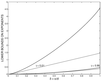
Figure 4: A comparison of the exponents of the bound in Corollary 4 and the particularized bound (83) from [11, Theorem 2.23]. This comparison is done for both $\gamma=0.01$ and $0.99$. The solid curves refer to the exponents of the bound in Corollary 4, and the dashed curves refer to the exponents of the looser bound in (83). The upper pair of curves refers to the exponents for $\gamma=0.01$, and the lower pair of curves (that approximately coincide) refers to the exponents for $\gamma=0.99$.

Consider, on the other hand, the probability of an event $\{|X_{n}-X_{0}|\geq\alpha\sqrt{n}\}$ where $\alpha\geq 0$ is arbitrary. It was shown in Appendix D that the optimized value of $x$ for the bound in Corollary 4 (and its generalized version in Theorem 42) scales like $\frac{1}{\sqrt{n}}$. Hence, it is approximately zero for $n\gg 1$, and $u\triangleq\gamma(e^{x}-1-x)\approx\frac{\gamma x^{2}}{2}$ scales like $\frac{1}{n}$. It therefore follows that $(1+u)^{n}\approx e^{nu}$ for $n\gg 1$. Moreover, the restriction on $x$ to be less than 3 in (86) does not affect the tightness of the bound in this case since the optimized value of $x$ is anyway close to zero. This explains the observation that the two bounds in Proposition 4 and [11, Theorem 2.23] essentially scale similarly for small deviations, where the probability of an event $\{|X_{n}-X_{0}|\geq\alpha\sqrt{n}\}$ for $\alpha\geq 0$ is considered.

V Applications in Information Theory and Related Topics

The refined versions of Azuma’s inequality in Section III are exemplified in this section to hypothesis testing and information theory, communication and coding.

V-A Binary Hypothesis Testing

Binary hypothesis testing for finite alphabet models was analyzed via the method of types, e.g., in [13, Chapter 11] and [14]. It is assumed that the data sequence is of a fixed length $(n)$, and one wishes to make the optimal decision (based on the Neyman-Pearson ratio test) based on the received sequence.

Let the RVs $X_{1},X_{2}....$ be i.i.d. $\sim Q$, and consider two hypotheses:

• $H_{1}:Q=P_{1}$.

• $H_{2}:Q=P_{2}$.

For the simplicity of the analysis, let us assume that the RVs are discrete, and take their values on a finite alphabet $\mathcal{X}$ where $P_{1}(x),P_{2}(x)>0$ for every $x\in\mathcal{X}$.

In the following, let

$$L(X_{1},\ldots,X_{n})\triangleq\ln\frac{P_{1}^{n}(X_{1},\ldots,X_{n})}{P_{2}^{n}(X_{1},\ldots,X_{n})}=\sum_{i=1}^{n}\ln\frac{P_{1}(X_{i})}{P_{2}(X_{i})}$$

designate the log-likelihood ratio. By the strong law of large number (SLLN), if hypothesis $H_{1}$ is true, then a.s.

$$\lim_{n\rightarrow\infty}\frac{L(X_{1},\ldots,X_{n})}{n}=D(P_{1}||P_{2})$$ (87)

and otherwise, if hypothesis $H_{2}$ is true, then a.s.

$$\lim_{n\rightarrow\infty}\frac{L(X_{1},\ldots,X_{n})}{n}=-D(P_{2}||P_{1})$$ (88)

where the above assumptions on the probability mass functions $P_{1}$ and $P_{2}$ imply that the relative entropies, $D(P_{1}||P_{2})$ and $D(P_{2}||P_{1})$, are both finite. Consider the case where for some fixed constants $\overline{\lambda},\underline{\lambda}\in\mathbb{R}$ where

$$-D(P_{2}||P_{1})<\underline{\lambda}\leq\overline{\lambda}<D(P_{1}||P_{2})$$

one decides on hypothesis $H_{1}$ if

$$L(X_{1},\ldots,X_{n})>n\overline{\lambda}$$

and on hypothesis $H_{2}$ if

$$L(X_{1},\ldots,X_{n})<n\underline{\lambda}.$$

Note that if $\overline{\lambda}=\underline{\lambda}\triangleq\lambda$ then a decision on the two hypotheses is based on comparing the normalized log-likelihood ratio (w.r.t. $n$) to a single threshold $(\lambda)$, and deciding on hypothesis $H_{1}$ or $H_{2}$ if this normalized log-likelihood ratio is, respectively, above or below $\lambda$. If $\underline{\lambda}<\overline{\lambda}$ then one decides on $H_{1}$ or $H_{2}$ if the normalized log-likelihood ratio is, respectively, above the upper threshold $\overline{\lambda}$ or below the lower threshold $\underline{\lambda}$. Otherwise, if the normalized log-likelihood ratio is between the upper and lower thresholds, then an erasure is declared and no decision is taken in this case.

Let

$$\alpha_{n}^{(1)}\triangleq P_{1}^{n}\Bigl{(}L(X_{1},\ldots,X_{n})\leq n\overline{\lambda}\Bigr{)}$$ (89)

$$\alpha_{n}^{(2)}\triangleq P_{1}^{n}\Bigl{(}L(X_{1},\ldots,X_{n})\leq n\underline{\lambda}\Bigr{)}$$ (90)

and

$$\beta_{n}^{(1)}\triangleq P_{2}^{n}\Bigl{(}L(X_{1},\ldots,X_{n})\geq n\underline{\lambda}\Bigr{)}$$ (91)

$$\beta_{n}^{(2)}\triangleq P_{2}^{n}\Bigl{(}L(X_{1},\ldots,X_{n})\geq n\overline{\lambda}\Bigr{)}$$ (92)

then $\alpha_{n}^{(1)}$ and $\beta_{n}^{(1)}$ are the probabilities of either making an error or declaring an erasure under, respectively, hypotheses $H_{1}$ and $H_{2}$; similarly $\alpha_{n}^{(2)}$ and $\beta_{n}^{(2)}$ are the probabilities of making an error under hypotheses $H_{1}$ and $H_{2}$, respectively.

Let $\pi_{1},\pi_{2}\in(0,1)$ denote the a-priori probabilities of the hypotheses $H_{1}$ and $H_{2}$, respectively, so

$$P_{\text{e},n}^{(1)}=\pi_{1}\alpha_{n}^{(1)}+\pi_{2}\beta_{n}^{(1)}$$ (93)

is the probability of having either an error or an erasure, and

$$P_{\text{e},n}^{(2)}=\pi_{1}\alpha_{n}^{(2)}+\pi_{2}\beta_{n}^{(2)}$$ (94)

is the probability of error.

V-A1 Exact Exponents

When we let $n$ tend to infinity, the exact exponents of $\alpha_{n}^{(j)}$ and $\beta_{n}^{(j)}$ ($j=1,2$) are derived via Cramér’s theorem. The resulting exponents form a straightforward generalization of, e.g., [16, Theorem 3.4.3] and [31, Theorem 6.4] that addresses the case where the decision is made based on a single threshold of the log-likelihood ratio. In this particular case where $\overline{\lambda}=\underline{\lambda}\triangleq\lambda$, the option of erasures does not exist, and $P_{\text{e},n}^{(1)}=P_{\text{e},n}^{(2)}\triangleq P_{\text{e},n}$ is the error probability.

In the considered general case with erasures, let

$$\lambda_{1}\triangleq-\overline{\lambda},\quad\lambda_{2}\triangleq-\underline{\lambda}$$

then Cramér’s theorem on $\mathbb{R}$ yields that the exact exponents of $\alpha_{n}^{(1)}$, $\alpha_{n}^{(2)}$, $\beta_{n}^{(1)}$ and $\beta_{n}^{(2)}$ are given by

$$\lim_{n\rightarrow\infty}-\frac{\ln\alpha_{n}^{(1)}}{n}=I(\lambda_{1})$$ (95)

$$\lim_{n\rightarrow\infty}-\frac{\ln\alpha_{n}^{(2)}}{n}=I(\lambda_{2})$$ (96)

$$\lim_{n\rightarrow\infty}-\frac{\ln\beta_{n}^{(1)}}{n}=I(\lambda_{2})-\lambda_{2}$$ (97)

$$\lim_{n\rightarrow\infty}-\frac{\ln\beta_{n}^{(2)}}{n}=I(\lambda_{1})-\lambda_{1}$$ (98)

where the rate function $I$ is given by

$$I(r)\triangleq\sup_{t\in\mathbb{R}}\bigl{(}tr-H(t)\bigr{)}$$ (99)

and

$$H(t)=\ln\Biggl{(}\sum_{x\in\mathcal{X}}P_{1}(x)^{1-t}P_{2}(x)^{t}\Biggr{)},\quad\forall\,t\in\mathbb{R}.$$ (100)

The rate function $I$ is convex, lower semi-continuous (l.s.c.) and non-negative (see, e.g., [16] and [31]). Note that

$$H(t)=(t-1)D_{t}(P_{2}||P_{1})$$

where $D_{t}(P||Q)$ designates Réyni’s information divergence of order $t$ [52, Eq. (3.3)], and $I$ in (99) is the Fenchel-Legendre transform of $H$ (see, e.g., [16, Definition 2.2.2]).

From (93)– (98), the exact exponents of $P_{\text{e},n}^{(1)}$ and $P_{\text{e},n}^{(2)}$ are equal to

$$\lim_{n\rightarrow\infty}-\frac{\ln P_{\text{e},n}^{(1)}}{n}=\min\Bigl{\{}I(\lambda_{1}),I(\lambda_{2})-\lambda_{2}\Bigr{\}}$$ (101)

and

$$\lim_{n\rightarrow\infty}-\frac{\ln P_{\text{e},n}^{(2)}}{n}=\min\Bigl{\{}I(\lambda_{2}),I(\lambda_{1})-\lambda_{1}\Bigr{\}}.$$ (102)

For the case where the decision is based on a single threshold for the log-likelihood ratio (i.e., $\lambda_{1}=\lambda_{2}\triangleq\lambda$), then $P_{\text{e},n}^{(1)}=P_{\text{e},n}^{(2)}\triangleq P_{\text{e},n}$, and its error exponent is equal to

$$\lim_{n\rightarrow\infty}-\frac{\ln P_{\text{e},n}}{n}=\min\Bigl{\{}I(\lambda),I(\lambda)-\lambda\Bigr{\}}$$ (103)

which coincides with the error exponent in [16, Theorem 3.4.3] (or [31, Theorem 6.4]). The optimal threshold for obtaining the best error exponent of the error probability $P_{\text{e},n}$ is equal to zero (i.e., $\lambda=0$); in this case, the exact error exponent is equal to

$$I(0)=-\min_{0\leq t\leq 1}\ln\Biggl{(}\sum_{x\in\mathcal{X}}P_{1}(x)^{1-t}P_{2}(x)^{t}\Biggr{)}$$

$$\hskip 19.91684pt\triangleq C(P_{1},P_{2})$$ (104)

which is the Chernoff information of the probability measures $P_{1}$ and $P_{2}$ (see [13, Eq. (11.239)]), and it is symmetric (i.e., $C(P_{1},P_{2})=C(P_{2},P_{1})$). Note that, from (99), $I(0)=\sup_{t\in\mathbb{R}}\bigl{(}-H(t)\bigr{)}=-\inf_{t\in\mathbb{R}}\bigl{(}H(t)\bigr{)}$; the minimization in (104) over the interval $[0,1]$ (instead of taking the infimum of $H$ over $\mathbb{R}$) is due to the fact that $H(0)=H(1)=0$ and the function $H$ in (100) is convex, so it is enough to restrict the infimum of $H$ to the closed interval $[0,1]$ for which it turns to be a minimum.

Paper [9] forms a classical paper that considers binary hypothesis testing from an information-theoretic point of view, and it derives the error exponents of binary hypothesis testers in analogy to optimum channel codes via the use of relative entropy measures. We will further explore on this kind of analogy in the continuation to this section (see later Sections V-A5 and V-A6 w.r.t. moderate and small deviations analysis of binary hypothesis testing).

V-A2 Lower Bound on the Exponents via Theorem 2

In the following, the tightness of Theorem 2 is examined by using it for the derivation of lower bounds on the error exponent and the exponent of the event of having either an error or an erasure. These results will be compared in the next sub-section to the exact exponents from the previous sub-section.

We first derive a lower bound on the exponent of $\alpha_{n}^{(1)}$. Under hypothesis $H_{1}$, let us construct the martingale sequence $\{U_{k},\mathcal{F}_{k}\}_{k=0}^{n}$ where $\mathcal{F}_{0}\subseteq\mathcal{F}_{1}\subseteq\ldots\mathcal{F}_{n}$ is the filtration

$$\mathcal{F}_{0}=\{\emptyset,\Omega\},\quad\mathcal{F}_{k}=\sigma(X_{1},\ldots,X_{k}),\;\;\forall\,k\in\{1,\ldots,n\}$$

and

$$U_{k}=\mathbb{E}_{P_{1}^{n}}\bigl{[}L(X_{1},\ldots,X_{n})\;|\;\mathcal{F}_{k}\bigr{]}.$$ (105)

For every $k\in\{0,\ldots,n\}$

$$U_{k}=\mathbb{E}_{P_{1}^{n}}\Biggl{[}\sum_{i=1}^{n}\ln\frac{P_{1}(X_{i})}{P_{2}(X_{i})}\;\Big{|}\;\mathcal{F}_{k}\Biggr{]}$$

$$\hskip 14.22636pt=\sum_{i=1}^{k}\ln\frac{P_{1}(X_{i})}{P_{2}(X_{i})}+\sum_{i=k+1}^{n}\mathbb{E}_{P_{1}^{n}}\Biggl{[}\ln\frac{P_{1}(X_{i})}{P_{2}(X_{i})}\Biggr{]}$$

$$\hskip 14.22636pt=\sum_{i=1}^{k}\ln\frac{P_{1}(X_{i})}{P_{2}(X_{i})}+(n-k)D(P_{1}||P_{2}).$$

In particular

$$U_{0}=nD(P_{1}||P_{2}),$$ (106)

$$U_{n}=\sum_{i=1}^{n}\ln\frac{P_{1}(X_{i})}{P_{2}(X_{i})}=L(X_{1},\ldots,X_{n})$$ (107)

and, for every $k\in\{1,\ldots,n\}$,

$$U_{k}-U_{k-1}=\ln\frac{P_{1}(X_{k})}{P_{2}(X_{k})}-D(P_{1}||P_{2}).$$ (108)

Let

$$d_{1}\triangleq\max_{x\in\mathcal{X}}\left|\ln\frac{P_{1}(x)}{P_{2}(x)}-D(P_{1}||P_{2})\right|$$ (109)

so $d_{1}<\infty$ since by assumption the alphabet set $\mathcal{X}$ is finite, and $P_{1}(x),P_{2}(x)>0$ for every $x\in\mathcal{X}$. From (108) and (109)

$$|U_{k}-U_{k-1}|\leq d_{1}$$

holds a.s. for every $k\in\{1,\ldots,n\}$, and

$$\mathbb{E}_{P_{1}^{n}}\bigl{[}(U_{k}-U_{k-1})^{2}\,|\,\mathcal{F}_{k-1}\bigr{]}$$

$$=\mathbb{E}_{P_{1}}\left[\left(\ln\frac{P_{1}(X_{k})}{P_{2}(X_{k})}-D(P_{1}||P_{2})\right)^{2}\right]$$

$$=\sum_{x\in\mathcal{X}}\left\{P_{1}(x)\left(\ln\frac{P_{1}(x)}{P_{2}(x)}-D(P_{1}||P_{2})\right)^{2}\right\}$$

$$\triangleq\sigma_{1}^{2}.$$ (110)

Let

$$\varepsilon_{1,1}=D(P_{1}||P_{2})-\overline{\lambda},\quad\varepsilon_{2,1}=D(P_{2}||P_{1})+\underline{\lambda}$$ (111)

$$\varepsilon_{1,2}=D(P_{1}||P_{2})-\underline{\lambda},\quad\varepsilon_{2,2}=D(P_{2}||P_{1})+\overline{\lambda}$$ (112)

The probability of making an erroneous decision on hypothesis $H_{2}$ or declaring an erasure under the hypothesis $H_{1}$ is equal to $\alpha_{n}^{(1)}$, and from Theorem 2

$$\alpha_{n}^{(1)}\triangleq P_{1}^{n}\bigl{(}L(X_{1},\ldots,X_{n})\leq n\overline{\lambda}\bigr{)}$$

$$\hskip 19.91684pt\stackrel{{\scriptstyle\text{(a)}}}{{=}}P_{1}^{n}(U_{n}-U_{0}\leq-\varepsilon_{1,1}\,n)$$ (113)

$$\hskip 19.91684pt\stackrel{{\scriptstyle\text{(b)}}}{{\leq}}\exp\left(-n\,D\Bigl{(}\frac{\delta_{1,1}+\gamma_{1}}{1+\gamma_{1}}\Big{|}\Big{|}\frac{\gamma_{1}}{1+\gamma_{1}}\Bigr{)}\right)$$ (114)

where equality (a) follows from (106), (107) and (111), and inequality (b) follows from Theorem 2 with

$$\gamma_{1}\triangleq\frac{\sigma_{1}^{2}}{d_{1}^{2}},\quad\delta_{1,1}\triangleq\frac{\varepsilon_{1,1}}{d_{1}}.$$ (115)

Note that if $\varepsilon_{1,1}>d_{1}$ then it follows from (108) and (109) that $\alpha_{n}^{(1)}$ is zero; in this case $\delta_{1,1}>1$, so the divergence in (114) is infinity and the upper bound is also equal to zero. Hence, it is assumed without loss of generality that $\delta_{1,1}\in[0,1]$.

Similarly to (105), under hypothesis $H_{2}$, let us define the martingale sequence $\{U_{k},\mathcal{F}_{k}\}_{k=0}^{n}$ with the same filtration and

$$U_{k}=\mathbb{E}_{P_{2}^{n}}\bigl{[}L(X_{1},\ldots,X_{n})\;|\;\mathcal{F}_{k}\bigr{]},\quad\forall\,k\in\{0,\ldots,n\}.$$ (116)

For every $k\in\{0,\ldots,n\}$

$$U_{k}=\sum_{i=1}^{k}\ln\frac{P_{1}(X_{i})}{P_{2}(X_{i})}-(n-k)D(P_{2}||P_{1})$$

and in particular

$$U_{0}=-nD(P_{2}||P_{1}),\quad U_{n}=L(X_{1},\ldots,X_{n}).$$ (117)

For every $k\in\{1,\ldots,n\}$,

$$U_{k}-U_{k-1}=\ln\frac{P_{1}(X_{k})}{P_{2}(X_{k})}+D(P_{2}||P_{1}).$$ (118)

Let

$$d_{2}\triangleq\max_{x\in\mathcal{X}}\left|\ln\frac{P_{2}(x)}{P_{1}(x)}-D(P_{2}||P_{1})\right|$$ (119)

then, the jumps of the latter martingale sequence are uniformly bounded by $d_{2}$ and, similarly to (110), for every $k\in\{1,\ldots,n\}$

$$\mathbb{E}_{P_{2}^{n}}\bigl{[}(U_{k}-U_{k-1})^{2}\,|\,\mathcal{F}_{k-1}\bigr{]}$$

$$=\sum_{x\in\mathcal{X}}\left\{P_{2}(x)\left(\ln\frac{P_{2}(x)}{P_{1}(x)}-D(P_{2}||P_{1})\right)^{2}\right\}$$

$$\triangleq\sigma_{2}^{2}.$$ (120)

Hence, it follows from Theorem 2 that

$$\beta_{n}^{(1)}\triangleq P_{2}^{n}\bigl{(}L(X_{1},\ldots,X_{n})\geq n\underline{\lambda}\bigr{)}$$

$$\hskip 19.91684pt=P_{2}^{n}(U_{n}-U_{0}\geq\varepsilon_{2,1}\,n)$$ (121)

$$\hskip 19.91684pt\leq\exp\left(-n\,D\Bigl{(}\frac{\delta_{2,1}+\gamma_{2}}{1+\gamma_{2}}\Big{|}\Big{|}\frac{\gamma_{2}}{1+\gamma_{2}}\Bigr{)}\right)$$ (122)

where the equality in (121) holds due to (117) and (111), and (122) follows from Theorem 2 with

$$\gamma_{2}\triangleq\frac{\sigma_{2}^{2}}{d_{2}^{2}},\quad\delta_{2,1}\triangleq\frac{\varepsilon_{2,1}}{d_{2}}$$ (123)

and $d_{2}$, $\sigma_{2}$ are introduced, respectively, in (119) and (120).

From (93), (114) and (122), the exponent of the probability of either having an error or an erasure is lower bounded by

$$\lim_{n\rightarrow\infty}-\frac{\ln P_{\text{e},n}^{(1)}}{n}\geq\min_{i=1,2}D\Bigl{(}\frac{\delta_{i,1}+\gamma_{i}}{1+\gamma_{i}}\Big{|}\Big{|}\frac{\gamma_{i}}{1+\gamma_{i}}\Bigr{)}.$$ (124)

Similarly to the above analysis, one gets from (94) and (112) that the error exponent is lower bounded by

$$\lim_{n\rightarrow\infty}-\frac{\ln P_{\text{e},n}^{(2)}}{n}\geq\min_{i=1,2}D\Bigl{(}\frac{\delta_{i,2}+\gamma_{i}}{1+\gamma_{i}}\Big{|}\Big{|}\frac{\gamma_{i}}{1+\gamma_{i}}\Bigr{)}$$ (125)

where

$$\delta_{1,2}\triangleq\frac{\varepsilon_{1,2}}{d_{1}},\quad\delta_{2,2}\triangleq\frac{\varepsilon_{2,2}}{d_{2}}.$$ (126)

For the case of a single threshold (i.e., $\overline{\lambda}=\underline{\lambda}\triangleq\lambda$) then (124) and (125) coincide, and one obtains that the error exponent satisfies

$$\lim_{n\rightarrow\infty}-\frac{\ln P_{\text{e},n}}{n}\geq\min_{i=1,2}D\Bigl{(}\frac{\delta_{i}+\gamma_{i}}{1+\gamma_{i}}\Big{|}\Big{|}\frac{\gamma_{i}}{1+\gamma_{i}}\Bigr{)}$$ (127)

where $\delta_{i}$ is the common value of $\delta_{i,1}$ and $\delta_{i,2}$ (for $i=1,2$). In this special case, the zero threshold is optimal (see, e.g., [16, p. 93]), which then yields that (127) is satisfied with

$$\delta_{1}=\frac{D(P_{1}||P_{2})}{d_{1}},\quad\delta_{2}=\frac{D(P_{2}||P_{1})}{d_{2}}$$ (128)

with $d_{1}$ and $d_{2}$ from (109) and (119), respectively. The right-hand side of (127) forms a lower bound on Chernoff information which is the exact error exponent for this special case.

V-A3 Comparison of the Lower Bounds on the Exponents with those that Follow from Azuma’s Inequality

The lower bounds on the error exponent and the exponent of the probability of having either errors or erasures, that were derived in the previous sub-section via Theorem 2, are compared in the following to the loosened lower bounds on these exponents that follow from Azuma’s inequality.

We first obtain upper bounds on $\alpha_{n}^{(1)},\alpha_{n}^{(2)},\beta_{n}^{(1)}$ and $\beta_{n}^{(2)}$ via Azuma’s inequality, and then use them to derive lower bounds on the exponents of $P_{\text{e},n}^{(1)}$ and $P_{\text{e},n}^{(2)}$.

From (108), (109), (113), (115), and Azuma’s inequality

$$\alpha_{n}^{(1)}\leq\exp\biggl{(}-\frac{\delta_{1,1}^{2}n}{2}\biggr{)}$$ (129)

and, similarly, from (118), (119), (121), (123), and Azuma’s inequality

$$\beta_{n}^{(1)}\leq\exp\biggl{(}-\frac{\delta_{2,1}^{2}n}{2}\biggr{)}.$$ (130)

From (90), (92), (112), (126) and Azuma’s inequality

$$\alpha_{n}^{(2)}\leq\exp\biggl{(}-\frac{\delta_{1,2}^{2}n}{2}\biggr{)}$$ (131)

$$\beta_{n}^{(2)}\leq\exp\biggl{(}-\frac{\delta_{2,2}^{2}n}{2}\biggr{)}.$$ (132)

Therefore, it follows from (93), (94) and (129)–(132) that the resulting lower bounds on the exponents of $P_{\text{e},n}^{(1)}$ and $P_{\text{e},n}^{(2)}$ are

$$\lim_{n\rightarrow\infty}-\frac{\ln P_{\text{e},n}^{(j)}}{n}\geq\min_{i=1,2}\frac{\delta_{i,j}^{2}}{2},\quad j=1,2$$ (133)

as compared to (124) and (125) which give, for $j=1,2$,

$$\lim_{n\rightarrow\infty}-\frac{\ln P_{\text{e},n}^{(j)}}{n}\geq\min_{i=1,2}D\Bigl{(}\frac{\delta_{i,j}+\gamma_{i}}{1+\gamma_{i}}\Big{|}\Big{|}\frac{\gamma_{i}}{1+\gamma_{i}}\Bigr{)}.$$ (134)

For the specific case of a zero threshold, the lower bound on the error exponent which follows from Azuma’s inequality is given by

$$\lim_{n\rightarrow\infty}-\frac{\ln P_{\text{e},n}^{(j)}}{n}\geq\min_{i=1,2}\frac{\delta_{i}^{2}}{2}$$ (135)

with the values of $\delta_{1}$ and $\delta_{2}$ in (128).

The lower bounds on the exponents in (133) and (134) are compared in the following. Note that the lower bounds in (133) are loosened as compared to those in (134) since they follow, respectively, from Azuma’s inequality and its improvement in Theorem 2.

The divergence in the exponent of (134) is equal to

$$D\Bigl{(}\frac{\delta_{i,j}+\gamma_{i}}{1+\gamma_{i}}\Big{|}\Big{|}\frac{\gamma_{i}}{1+\gamma_{i}}\Bigr{)}$$

$$=\left(\frac{\delta_{i,j}+\gamma_{i}}{1+\gamma_{i}}\right)\ln\left(1+\frac{\delta_{i,j}}{\gamma_{i}}\right)+\left(\frac{1-\delta_{i,j}}{1+\gamma_{i}}\right)\ln(1-\delta_{i,j})$$

$$=\frac{\gamma_{i}}{1+\gamma_{i}}\left[\left(1+\frac{\delta_{i,j}}{\gamma_{i}}\right)\ln\Bigl{(}1+\frac{\delta_{i,j}}{\gamma_{i}}\Bigr{)}+\frac{(1-\delta_{i,j})\ln(1-\delta_{i,j})}{\gamma_{i}}\right].$$

(136)

Lemma 3

$$(1+u)\ln(1+u)\geq\left\{\begin{array}[]{ll}u+\frac{u^{2}}{2},&u\in[-1,0]\\[5.69046pt] u+\frac{u^{2}}{2}-\frac{u^{3}}{6},&u\geq 0\end{array}\right.$$ (137)

where at $u=-1$, the left-hand side is defined to be zero (it is the limit of this function when $u\rightarrow-1$ from above).

Proof:

The proof follows by elementary calculus. ∎

Since $\delta_{i,j}\in[0,1]$, then (136) and Lemma 3 imply that

$$D\Bigl{(}\frac{\delta_{i,j}+\gamma_{i}}{1+\gamma_{i}}\Big{|}\Big{|}\frac{\gamma_{i}}{1+\gamma_{i}}\Bigr{)}\geq\frac{\delta_{i,j}^{2}}{2\gamma_{i}}-\frac{\delta_{i,j}^{3}}{6\gamma_{i}^{2}(1+\gamma_{i})}.$$ (138)

Hence, by comparing (133) with the combination of (134) and (138), then it follows that (up to a second-order approximation) the lower bounds on the exponents that were derived via Theorem 2 are improved by at least a factor of $\bigl{(}\max\gamma_{i}\bigr{)}^{-1}$ as compared to those that follow from Azuma’s inequality.

Example 4

Consider two probability measures $P_{1}$ and $P_{2}$ where

$$P_{1}(0)=P_{2}(1)=0.4,\quad P_{1}(1)=P_{2}(0)=0.6,$$

and the case of a single threshold of the log-likelihood ratio that is set to zero (i.e., $\lambda=0$). The exact error exponent in this case is Chernoff information that is equal to

$$C(P_{1},P_{2})=2.04\cdot 10^{-2}.$$

The improved lower bound on the error exponent in (127) and (128) is equal to $1.77\cdot 10^{-2}$, whereas the loosened lower bound in (135) is equal to $1.39\cdot 10^{-2}$. In this case $\gamma_{1}=\frac{2}{3}$ and $\gamma_{2}=\frac{7}{9}$, so the improvement in the lower bound on the error exponent is indeed by a factor of approximately

$$\left(\max_{i}\gamma_{i}\right)^{-1}=\frac{9}{7}.$$

Note that, from (114), (122) and (129)–(132), these are lower bounds on the error exponents for any finite block length $n$, and not only asymptotically in the limit where $n\rightarrow\infty$. The operational meaning of this example is that the improved lower bound on the error exponent assures that a fixed error probability can be obtained based on a sequence of i.i.d. RVs whose length is reduced by 22.2% as compared to the loosened bound which follows from Azuma’s inequality.

V-A4 Comparison of the Exact and Lower Bounds on the Error Exponents, Followed by a Relation to Fisher Information

In the following, we compare the exact and lower bounds on the error exponents. Consider the case where there is a single threshold on the log-likelihood ratio (i.e., referring to the case where the erasure option is not provided) that is set to zero. The exact error exponent in this case is given by the Chernoff information (see (104)), and it will be compared to the two lower bounds on the error exponents that were derived in the previous two subsections.

Let $\{P_{\theta}\}_{\theta\in\Theta}$, denote an indexed family of probability mass functions where $\Theta$ denotes the parameter set. Assume that $P_{\theta}$ is differentiable in the parameter $\theta$. Then, the Fisher information is defined as

$$J(\theta)\triangleq\mathbb{E}_{\theta}\left[\frac{\partial}{\partial\theta}\,\ln P_{\theta}(x)\right]^{2}$$ (139)

where the expectation is w.r.t. the probability mass function $P_{\theta}$. The divergence and Fisher information are two related information measures, satisfying the equality

$$\lim_{\theta^{\prime}\rightarrow\theta}\frac{D(P_{\theta}||P_{\theta^{\prime}})}{(\theta-\theta^{\prime})^{2}}=\frac{J(\theta)}{2}$$ (140)

(note that if it was a relative entropy to base 2 then the right-hand side of (140) would have been divided by $\ln 2$, and be equal to $\frac{J(\theta)}{\ln 4}$ as in [13, Eq. (12.364)]).

Proposition 6

Under the above assumptions,

• The Chernoff information and Fisher information are related information measures that satisfy the equality

  $$\lim_{\theta^{\prime}\rightarrow\theta}\frac{C(P_{\theta},P_{\theta^{\prime}})}{(\theta-\theta^{\prime})^{2}}=\frac{J(\theta)}{8}.$$ (141)

• Let

  $$E_{\text{L}}(P_{\theta},P_{\theta^{\prime}})\triangleq\min_{i=1,2}D\Bigl{(}\frac{\delta_{i}+\gamma_{i}}{1+\gamma_{i}}\Big{|}\Big{|}\frac{\gamma_{i}}{1+\gamma_{i}}\Bigr{)}$$ (142)

  be the lower bound on the error exponent in (127) which corresponds to $P_{1}\triangleq P_{\theta}$ and $P_{2}\triangleq P_{\theta^{\prime}}$, then also

  $$\lim_{\theta^{\prime}\rightarrow\theta}\frac{E_{\text{L}}(P_{\theta},P_{\theta^{\prime}})}{(\theta-\theta^{\prime})^{2}}=\frac{J(\theta)}{8}.$$ (143)

• Let

  $$\widetilde{E}_{\text{L}}(P_{\theta},P_{\theta^{\prime}})\triangleq\min_{i=1,2}\frac{\delta_{i}^{2}}{2}$$ (144)

  be the loosened lower bound on the error exponent in (135) which refers to $P_{1}\triangleq P_{\theta}$ and $P_{2}\triangleq P_{\theta^{\prime}}$. Then,

  $$\lim_{\theta^{\prime}\rightarrow\theta}\frac{\widetilde{E}_{\text{L}}(P_{\theta},P_{\theta^{\prime}})}{(\theta-\theta^{\prime})^{2}}=\frac{a(\theta)\,J(\theta)}{8}$$ (145)

  for some deterministic function $a$ bounded in $[0,1]$, and there exists an indexed family of probability mass functions for which $a(\theta)$ can be made arbitrarily close to zero for any fixed value of $\theta\in\Theta$.

Proof:

See Appendix K. ∎

Proposition 6 shows that, in the considered setting, the refined lower bound on the error exponent provides the correct behavior of the error exponent for a binary hypothesis testing when the relative entropy between the pair of probability mass functions that characterize the two hypotheses tends to zero. This stays in contrast to the loosened error exponent, which follows from Azuma’s inequality, whose scaling may differ significantly from the correct exponent (for a concrete example, see the last part of the proof in Appendix K).

Example 5

Consider the index family of of probability mass functions defined over the binary alphabet $\mathcal{X}=\{0,1\}$:

$$P_{\theta}(0)=1-\theta,\;\;P_{\theta}(1)=\theta,\quad\forall\,\theta\in(0,1).$$

From (139), the Fisher information is equal to

$$J(\theta)=\frac{1}{\theta}+\frac{1}{1-\theta}$$

and, at the point $\theta=0.5$, $J(\theta)=4$. Let $\theta_{1}=0.51$ and $\theta_{2}=0.49$, so from (141) and (143)

$$C(P_{\theta_{1}},P_{\theta_{2}}),E_{\text{L}}(P_{\theta_{1}},P_{\theta_{2}})\approx\frac{J(\theta)(\theta_{1}-\theta_{2})^{2}}{8}=2.00\cdot 10^{-4}.$$

Indeed, the exact values of $C(P_{\theta_{1}},P_{\theta_{2}})$ and $E_{\text{L}}(P_{\theta_{1}},P_{\theta_{2}})$ are $2.000\cdot 10^{-4}$ and $1.997\cdot 10^{-4}$, respectively.

V-A5 Moderate Deviations Analysis for Binary Hypothesis Testing

So far, we have discussed large deviations analysis for binary hypothesis testing, and compared the exact error exponents with lower bounds that follow from refined versions of Azuma’s inequality.

Based on the asymptotic results in (87) and (88), which hold a.s. under hypotheses $H_{1}$ and $H_{2}$ respectively, the large deviations analysis refers to upper and lower thresholds $\overline{\lambda}$ and $\underline{\lambda}$ which are kept fixed (i.e., these thresholds do not depend on the block length $n$ of the data sequence) where

$$-D(P_{2}||P_{1})<\underline{\lambda}\leq\overline{\lambda}<D(P_{1}||P_{2}).$$

Suppose that instead of having some fixed upper and lower thresholds, one is interested to set these thresholds such that as the block length $n$ tends to infinity, they tend simultaneously to their asymptotic limits in (87) and (88), i.e.,

$$\lim_{n\rightarrow\infty}\overline{\lambda}^{(n)}=D(P_{1}||P_{2}),\quad\lim_{n\rightarrow\infty}\underline{\lambda}^{(n)}=-D(P_{2}||P_{1}).$$

Specifically, let $\eta\in(\frac{1}{2},1)$, and $\varepsilon_{1},\varepsilon_{2}>0$ be arbitrary fixed numbers, and consider the case where one decides on hypothesis $H_{1}$ if

$$L(X_{1},\ldots,X_{n})>n\overline{\lambda}^{(n)}$$

and on hypothesis $H_{2}$ if

$$L(X_{1},\ldots,X_{n})<n\underline{\lambda}^{(n)}$$

where these upper and lower thresholds are set to

$$\overline{\lambda}^{(n)}=D(P_{1}||P_{2})-\varepsilon_{1}n^{-(1-\eta)}$$

$$\underline{\lambda}^{(n)}=-D(P_{2}||P_{1})+\varepsilon_{2}n^{-(1-\eta)}$$

so that they approach, respectively, the relative entropies $D(P_{1}||P_{2})$ and $-D(P_{2}||P_{1})$ in the asymptotic case where the block length $n$ of the data sequence tends to infinity. Accordingly, the conditional probabilities in (89)–(92) are modified so that the fixed thresholds $\overline{\lambda}$ and $\underline{\lambda}$ are replaced with the above block-length dependent thresholds $\overline{\lambda}^{(n)}$ and $\underline{\lambda}^{(n)}$, respectively. The moderate deviations analysis for binary hypothesis testing studies the probability of an error event and the probability of a joint error and erasure event under the two hypotheses, and it studies the interplay between each of these probabilities, the block length $n$, and the related thresholds that tend asymptotically to the limits in (87) and (88) when the block length tends to infinity.

Before proceeding to the moderate deviations analysis for binary hypothesis testing, the related literature is reviewed shortly. As was noted in [2], moderate deviations analysis appears so far in the information theory literature only in two recent works: Moderate deviations behavior of channel coding for discrete memoryless channels was studied in [2], with direct and converse results which explicitly characterize the rate function of the moderate deviations principle (MDP). In their considered analysis, the authors of [2] studied the interplay between the probability of error, code rate and block length when the communication takes place over discrete memoryless channels, having the interest to figure out how the error probability of the best code scales when simultaneously the block length tends to infinity and the code rate approaches the channel capacity. The novelty in the setup of their analysis was the consideration of the scenario mentioned above, in contrast to the case where the rate is kept fixed below capacity, and the study is reduced to a characterization of the dependence between the two remaining parameters (i.e., the block length $n$ and the average/ maximal error probability of the best code). As opposed to the latter case, which corresponds to large deviations analysis and implies a characterization of error exponents as a function of the fixed rate, the analysis made in [2] (via the introduction of direct and converse theorems) demonstrated a sub-exponential scaling of the maximal error probability in the considered moderate deviations regime. In another recent paper [28], the moderate deviations analysis of the Slepian-Wolf problem was studied, and to the best of our knowledge, the authors of [28] were the first to consider moderate deviations analysis in the information theory literature. In the probability literature, moderate deviations analysis was extensively studied (see, e.g., [16, Section 3.7]), and in particular the MDP was studied in [15] in the context of continuous-time martingales with bounded jumps.

In light of the discussion in Section IV-F on the MDP for i.i.d. RVs and the discussion of its relation to the concentration inequalities in Section III (see Appendix J), and also motivated by the two recent works in [2] and [28], we proceed to consider in the following moderate deviations analysis for binary hypothesis testing. Our approach for this kind of analysis relies on concentration inequalities for martingales.

In the following, we analyze the probability of a joint error and erasure event under hypothesis $H_{1}$, i.e., derive an upper bound on $\alpha_{n}^{(1)}$ in (89). The same kind of analysis can be adapted easily for the other probabilities in (90)–(92). As mentioned earlier, let $\varepsilon_{1}>0$ and $\eta\in(\frac{1}{2},1)$ be arbitrarily fixed numbers. Then, under hypothesis $H_{1}$, it follows that similarly to (113)–(115)

$$P_{1}^{n}\bigl{(}L(X_{1},\ldots,X_{n})\leq n\overline{\lambda}^{(n)})$$

$$=P_{1}^{n}\bigl{(}L(X_{1},\ldots,X_{n})\leq nD(P_{1}||P_{2})-\varepsilon_{1}n^{\eta}\bigr{)}$$

$$\leq\exp\left(-nD\biggl{(}\frac{\delta_{1}^{(\eta,n)}+\gamma_{1}}{1+\gamma_{1}}\,\big{|}\big{|}\,\frac{\gamma_{1}}{1+\gamma_{1}}\biggr{)}\right)$$ (146)

where

$$\delta_{1}^{(\eta,n)}\triangleq\frac{\varepsilon_{1}n^{-(1-\eta)}}{d_{1}},\quad\gamma_{1}\triangleq\frac{\sigma_{1}^{2}}{d_{1}^{2}}$$ (147)

with $d_{1}$ and $\sigma_{1}^{2}$ from (109) and (110). From (136), (137) and (147), it follows that

$$D\biggl{(}\frac{\delta_{1}^{(\eta,n)}+\gamma_{1}}{1+\gamma_{1}}\,\big{|}\big{|}\,\frac{\gamma_{1}}{1+\gamma_{1}}\biggr{)}$$

$$=\frac{\gamma_{1}}{1+\gamma_{1}}\left[\Bigl{(}1+\frac{\delta_{1}^{(\eta,n)}}{\gamma_{1}}\Bigr{)}\ln\Bigl{(}1+\frac{\delta_{1}^{(\eta,n)}}{\gamma_{1}}\Bigr{)}\right.$$

$$\hskip 42.67912pt\left.+\frac{\bigl{(}1-\delta_{1}^{(\eta,n)}\bigr{)}\ln\bigl{(}1-\delta_{1}^{(\eta,n)}\bigr{)}}{\gamma_{1}}\right]$$

$$\geq\frac{\gamma_{1}}{1+\gamma_{1}}\left[\biggl{(}\frac{\delta_{1}^{(\eta,n)}}{\gamma_{1}}+\frac{\bigl{(}\delta_{1}^{(\eta,n)}\bigr{)}^{2}}{2\gamma_{1}^{2}}-\frac{\bigl{(}\delta_{1}^{(\eta,n)}\bigr{)}^{3}}{6\gamma_{1}^{3}}\biggr{)}\right.$$

$$\hskip 42.67912pt\left.+\frac{1}{\gamma_{1}}\biggl{(}-\delta_{1}^{(\eta,n)}+\frac{(\delta_{1}^{(\eta,n)})^{2}}{2}\biggr{)}\right]$$

$$=\frac{\bigl{(}\delta_{1}^{(\eta,n)}\bigr{)}^{2}}{2\gamma_{1}}-\frac{\bigl{(}\delta_{1}^{(\eta,n)}\bigr{)}^{3}}{6\gamma_{1}^{2}(1+\gamma_{1})}$$

$$=\frac{\varepsilon_{1}^{2}\,n^{-2(1-\eta)}}{2\gamma_{1}d_{1}^{2}}\left(1-\frac{\varepsilon_{1}}{3d_{1}\gamma_{1}(1+\gamma_{1})}\,\frac{1}{n^{1-\eta}}\right)$$

$$=\frac{\varepsilon_{1}^{2}\,n^{-2(1-\eta)}}{2\sigma_{1}^{2}}\left(1-\frac{\varepsilon_{1}d_{1}}{3\sigma_{1}^{2}(1+\gamma_{1})}\,\frac{1}{n^{1-\eta}}\right)$$

provided that $\delta_{1}^{(\eta,n)}<1$ (which holds for $n\geq n_{0}$ for some $n_{0}\triangleq n_{0}(\eta,\varepsilon_{1},d_{1})\in\mathbb{N}$ that is determined from (147)). By substituting this lower bound on the divergence into (146), it follows that

$$P_{1}^{n}\bigl{(}L(X_{1},\ldots,X_{n})\leq nD(P_{1}||P_{2})-\varepsilon_{1}n^{\eta}\bigr{)}$$

$$\leq\exp\left(-\frac{\varepsilon_{1}^{2}\,n^{2\eta-1}}{2\sigma_{1}^{2}}\left(1-\frac{\varepsilon_{1}d_{1}}{3\sigma_{1}^{2}(1+\gamma_{1})}\,\frac{1}{n^{1-\eta}}\right)\right)$$ (148)

so this upper bound has a sub-exponential decay to zero. In particular, in the limit where $n$ tends to infinity

$$\lim_{n\rightarrow\infty}n^{2\eta-1}\ln\,P_{1}^{n}\bigl{(}L(X_{1},\ldots,X_{n})\leq nD(P_{1}||P_{2})-\varepsilon_{1}n^{\eta}\bigr{)}$$

$$\leq-\frac{\varepsilon_{1}^{2}}{2\sigma_{1}^{2}}$$ (149)

with $\sigma_{1}^{2}$ in (110), i.e.,

$$\sigma_{1}^{2}\triangleq\sum_{x\in\mathcal{X}}\left\{P_{1}(x)\left(\ln\frac{P_{1}(x)}{P_{2}(x)}-D(P_{1}||P_{2})\right)^{2}\right\}.$$

From the analysis in Section IV-F and Appendix J, the following things hold:

• The inequality for the asymptotic limit in (149) holds in fact with equality.

• The same asymptotic result also follows from Theorem 42 for every even-valued $m\geq 2$ (instead of Theorem 2).

To verify these statements, consider the real-valued sequence of i.i.d. RVs

$$Y_{i}\triangleq\ln\left(\frac{P_{1}(X_{i})}{P_{2}(X_{i})}\right)-D(P_{1}||P_{2}),\quad i=1,\dots,n$$

that, under hypothesis $H_{1}$, have zero mean and variance $\sigma_{1}^{2}$. Since, by assumption, the sequence $\{X_{i}\}_{i=1}^{n}$ are i.i.d., then

$$L(X_{1},\ldots,X_{n})-nD(P_{1}||P_{2})=\sum_{i=1}^{n}Y_{i},$$ (150)

and it follows from the one-sided version of the MDP in (79) that indeed (149) holds with equality. Moreover, Theorem 2 provides, via the inequality in (148), a finite-length result that enhances the asymptotic result for $n\rightarrow\infty$. The second item above follows from the second part of the analysis in Appendix J (i.e., the part of analysis in this appendix that follows from Theorem 42).

A completely similar analysis w.r.t. moderate deviations for binary hypothesis testing can be also performed under hypothesis $H_{2}$. Note that, in the considered setting of moderate deviations analysis for binary hypothesis testing, the error probability has a sub-exponential decay to zero that is similar to the scaling that was obtained in [2] by the moderate deviations analysis for channel coding.

V-A6 Second-Order Analysis for Binary Hypothesis Testing

The moderate deviations analysis in the previous sub-section refers to deviations that scale like $n^{\eta}$ for $\eta\in(\frac{1}{2},1)$. Let us consider now the case of $\eta=\frac{1}{2}$ which corresponds to small deviations. To this end, refer to the real-valued sequence of i.i.d. RVs $\{Y_{i}\}_{i=1}^{n}$ with zero mean and variance $\sigma_{1}^{2}$ (under hypothesis $H_{1}$), and define the partial sums $S_{k}=\sum_{i=1}^{k}Y_{i}$ for $k\in\{1,\ldots,n\}$ with $S_{0}=0$. This implies that $\{S_{k},\mathcal{F}_{k}\}_{k=0}^{n}$ is a martingale-difference sequence. At this point, it links the current discussion on binary hypothesis testing to Section IV-D which refers to the relation between the martingale CLT and Proposition 4. Specifically, since from (150),

$$S_{n}-S_{0}=L(X_{1},\ldots,X_{n})-nD(P_{1}||P_{2})$$

then from the proof of Proposition 4, one gets an upper bound on the probability

$$P_{1}^{n}\bigl{(}L(X_{1},\ldots,X_{n})\leq nD(P_{1}||P_{2})-\varepsilon_{1}\sqrt{n}\bigr{)}$$

for a finite block length $n$ (via an analysis that is either related to Theorem 2 or 42) which agrees with the asymptotic result

$$\lim_{n\rightarrow\infty}\ln\,P_{1}^{n}\bigl{(}L(X_{1},\ldots,X_{n})\leq nD(P_{1}||P_{2})-\varepsilon_{1}\sqrt{n}\bigr{)}$$

$$=-\frac{\varepsilon_{1}^{2}}{2\sigma_{1}^{2}}.$$ (151)

Referring to small deviations analysis and the CLT, it shows a duality between these kind of results and recent works on second-order analysis for channel coding (see [29], [49], [50] and [51], where the variance $\sigma_{1}^{2}$ in (110) is replaced with the channel dispersion that is defined to be the variance of the mutual information RV between the channel input and output, and is a property of the communication channel solely).

V-B Pairwise Error Probability for Linear Block Codes over Binary-Input Output-Symmetric DMCs

In this sub-section, the tightness of Theorems 2 and 42 is studied by the derivation of upper bounds on the pairwise error probability under maximum-likelihood (ML) decoding when the transmission takes place over a discrete memoryless channel (DMC).

Let $\mathcal{C}$ be a binary linear block code of block length $n$, and assume that the codewords are a-priori equi-probable. Consider the case where the communication takes place over a binary-input output-symmetric DMC whose input alphabet is $\mathcal{X}=\{0,1\}$, and its output alphabet $\mathcal{Y}$ is finite.

In the following, boldface letters denote vectors, regular letters with sub-scripts denote individual elements of vectors, capital letters represent RVs, and lower-case letters denote individual realizations of the corresponding RVs. Let

$$P_{{\bf{Y}}|{\bf{X}}}(\underline{y}|\underline{x})=\prod_{i=1}^{n}P_{Y|X}(y_{i}|x_{i})$$

be the transition probability of the DMC, where due to the symmetry assumption

$$P_{Y|X}(y|0)=P_{Y|X}(-y|1),\quad\forall\,y\in\mathcal{Y}.$$

It is also assumed in the following that $P_{Y|X}(y|x)>0$ for every $(x,y)\in\mathcal{X}\times\mathcal{Y}$. Due to the linearity of the code and the symmetry of the DMC, the decoding error probability is independent of the transmitted codeword, so it is assumed without any loss of generality that the all-zero codeword is transmitted. In the following, we consider the pairwise error probability when the competitive codeword $\underline{x}\in\mathcal{C}$ has a Hamming weight that is equal to $h$, and denote it by $W_{\text{H}}(\underline{x})=h$. Let $P_{\bf{Y}}$ denote the probability distribution of the channel output.

In order to derive upper bounds on the pairwise error probability, let us define the following two hypotheses:

• $H_{1}:\;P_{\bf{Y}}(\underline{y})=\prod_{i=1}^{n}P_{Y|X}(y_{i}|0),\quad\forall\underline{y}\in\mathcal{Y}^{n},$
  

• $H_{2}:\;P_{\bf{Y}}(\underline{y})=\prod_{i=1}^{n}P_{Y|X}(y_{i}|x_{i}),\quad\forall\underline{y}\in\mathcal{Y}^{n}$

which correspond, respectively, to the transmission of the all-zero codeword and the competitive codeword $\underline{x}\in\mathcal{C}$.

Under hypothesis $H_{1}$, the considered pairwise error event under ML decoding occurs if and only if

$$\sum_{i=1}^{n}\ln\left(\frac{P_{Y|X}(y_{i}|x_{i})}{P_{Y|X}(y_{i}|0)}\right)\geq 0.$$

Let $\{i_{k}\}_{k=1}^{h}$ be the $h$ indices of the coordinates of $\underline{x}$ where $x_{i}=1$, ordered such that $1\leq i_{1}<\ldots<i_{h}\leq n$. Based on this notation, the log-likelihood ratio satisfies the equality

$$\sum_{i=1}^{n}\ln\left(\frac{P_{Y|X}(y_{i}|x_{i})}{P_{Y|X}(y_{i}|0)}\right)=\sum_{m=1}^{h}\ln\left(\frac{P_{Y|X}(y_{i_{m}}|1)}{P_{Y|X}(y_{i_{m}}|0)}\right).$$ (152)

For the continuation of the analysis in this sub-section, let us define the martingale sequence $\{U_{k},\mathcal{F}_{l}\}_{k=0}^{n}$ with the filtration

$$\mathcal{F}_{k}=\sigma(Y_{i_{1}},\ldots,Y_{i_{k}}),\quad k=1,\ldots,h$$

$$\mathcal{F}_{0}=\{\emptyset,\Omega\}$$

and, under hypothesis $H_{1}$, let

$$U_{k}=\mathbb{E}\left[\sum_{m=1}^{h}\ln\left(\frac{P_{Y|X}(Y_{i_{m}}|1)}{P_{Y|X}(Y_{i_{m}}|0)}\right)\,\Big{|}\,\mathcal{F}_{k}\right],\;\forall\,k\in\{0,1,\ldots,h\}.$$

Since, under hypothesis $H_{1}$, the RVs $Y_{i_{1}},\ldots,Y_{i_{h}}$ are statistically independent, then for $k\in\{0,1,\dots,h\}$

$$U_{k}=\sum_{m=1}^{k}\ln\left(\frac{P_{Y|X}(Y_{i_{m}}|1)}{P_{Y|X}(Y_{i_{m}}|0)}\right)$$

$$+(h-k)\sum_{y\in\mathcal{Y}}P_{Y|X}(y|0)\ln\left(\frac{P_{Y|X}(y|1)}{P_{Y|X}(y|0)}\right)$$

$$=\sum_{m=1}^{k}\ln\left(\frac{P_{Y|X}(Y_{i_{m}}|1)}{P_{Y|X}(Y_{i_{m}}|0)}\right)$$

$$-(h-k)\;D\bigl{(}P_{Y|X}(\cdot|0)\,||\,P_{Y|X}(\cdot|1)\bigr{)}.$$ (153)

Specifically

$$U_{0}=-h\,D\bigl{(}P_{Y|X}(\cdot|0)\,||\,P_{Y|X}(\cdot|1)\bigr{)}$$ (154)

$$U_{h}=\sum_{i=1}^{n}\ln\left(\frac{P_{Y|X}(Y_{i}|x_{i})}{P_{Y|X}(Y_{i}|0)}\right)$$ (155)

where the last equality follows from (152) and (153), and the differences of the martingale sequence are given by

$$\xi_{k}\triangleq U_{k}-U_{k-1}$$

$$=\ln\left(\frac{P_{Y|X}(Y_{i_{k}}|1)}{P_{Y|X}(Y_{i_{k}}|0)}\right)+D\bigl{(}P_{Y|X}(\cdot|0)\,||\,P_{Y|X}(\cdot|1)\bigr{)}$$ (156)

for every $k\in\{1,\ldots,h\}$. Note that, under hypothesis $H_{1}$, indeed $\mathbb{E}[\xi_{k}|\mathcal{F}_{k-1}]=0.$

The probability of a pairwise error event, where the ML decoder prefers a competitive codeword $\underline{x}\in\mathcal{C}$ ($W_{\text{H}}(\underline{x})=h$) over the transmitted all-zero codeword, is equal to

$$P_{h}\triangleq\mathbb{P}(U_{h}>0\;|\;H_{1})$$

$$=\mathbb{P}\Bigl{(}U_{h}-U_{0}>h\,D\bigl{(}P_{Y|X}(\cdot|0)\,||\,P_{Y|X}(\cdot|1)\bigr{)}\;|\;H_{1}\Bigr{)}.$$ (157)

It therefore follows that a.s. for every $k\in\{1,\ldots,h\}$

$$|\xi_{k}|\leq\max_{y\in\mathcal{Y}}\,\biggl{|}\,\ln\left(\frac{P_{Y|X}(y|1)}{P_{Y|X}(y|0)}\right)\biggr{|}+D\bigl{(}P_{Y|X}(\cdot|0)\,||\,P_{Y|X}(\cdot|1)\bigr{)}$$

$$\triangleq d<\infty$$ (158)

which is indeed finite since, by assumption, the alphabet $\mathcal{Y}$ is finite and $P_{Y|X}(y|x)>0$ for every $(x,y)\in\mathcal{X}\times\mathcal{Y}$. Note that, in fact, taking an absolute value in the maximization of the logarithm on the right-hand side of (158) is redundant due to the channel symmetry, and also due to the equality $\sum_{y}P_{Y|X}(y|0)=\sum_{y}P_{Y|X}(y|1)=1$ (so that it follows, from this equality, that there exists an element $y\in\mathcal{Y}$ such that $P_{Y|X}(y|1)\geq P_{Y|X}(y|0))$.

As an interim conclusion, $\{U_{k},\mathcal{F}_{k}\}_{k=0}^{h}$ is a martingale sequence with bounded jumps, and $|U_{k}-U_{k-1}|\leq d$ holds a.s. for every $k\in\{1,\ldots,h\}$. We rely in the following on the concentration inequalities of Theorems 2 and 42 to obtain, via (156)–(158), upper bounds on the pairwise error probability. The tightness of these bounds will be examined numerically, and they will be compared to the Bhattacharyya upper bound.

V-B1 Analysis Related to Theorem 2

From (156), for every $k\in\{1,\ldots,h\}$

$$\mathbb{E}[\xi_{k}^{2}|\mathcal{F}_{k-1}]$$

$$=\sum_{y\in\mathcal{Y}}P_{Y|X}(y|0)\biggl{[}\ln\left(\frac{P_{Y|X}(y|1)}{P_{Y|X}(y|0)}\right)$$

$$\hskip 14.22636pt+D\bigl{(}P_{Y|X}(\cdot|0)\,||\,P_{Y|X}(\cdot|1)\bigr{)}\biggr{]}^{2}$$

$$=\sum_{y\in\mathcal{Y}}P_{Y|X}(y|0)\biggl{[}\ln\left(\frac{P_{Y|X}(y|1)}{P_{Y|X}(y|0)}\right)\biggr{]}^{2}$$

$$-\Bigl{[}D\bigl{(}P_{Y|X}(\cdot|0)\,||\,P_{Y|X}(\cdot|1)\bigr{)}\Bigr{]}^{2}\triangleq\sigma^{2}$$ (159)

holds a.s., where the last equality follows from the definition of the divergence (relative entropy). Based on (157) and the notation in (11), let

$$\gamma=\frac{\sigma^{2}}{d^{2}},\quad\delta\triangleq\frac{D\bigl{(}P_{Y|X}(\cdot|0)\,||\,P_{Y|X}(\cdot|1)\bigr{)}}{d}$$ (160)

where $d$ and $\sigma^{2}$ are introduced in (158) and (159), respectively. Under hypothesis $H_{1}$, one gets from (157) and Theorem 2 that the pairwise error probability satisfies the upper bound

$$P_{h}\leq Z_{1}^{h}$$ (161)

where

$$Z_{1}\triangleq\exp\left(-D\Bigl{(}\frac{\delta+\gamma}{1+\gamma}\,\big{|}\big{|}\,\frac{\gamma}{1+\gamma}\Bigr{)}\right)$$ (162)

and $\gamma$, $\delta$ are introduced in (160).

In the following, we compare the exponential bound in (161) with the Bhattacharyya bound

$$P_{h}\leq Z_{\text{B}}^{h}$$ (163)

where the Bhattacharyya parameter $Z_{\text{B}}$ of the binary-input DMC is given by

$$Z_{\text{B}}\triangleq\sum_{y\in\mathcal{Y}}\sqrt{P_{Y|X}(y|0)P_{Y|X}(y|1)}\,.$$ (164)

Example 6

Consider a binary symmetric channel (BSC) with crossover probability $p$. The Bhattacharyya parameter which corresponds to this channel is $Z_{\text{B}}=\sqrt{4p(1-p)}$. In the following, $Z_{1}$ from (162) is calculated for comparison. Without loss of generality, assume that $p\leq\frac{1}{2}$. Straightforward calculation shows that

$$d=2(1-p)\ln\Bigl{(}\frac{1-p}{p}\Bigr{)}$$

$$\sigma^{2}=4p(1-p)\left[\ln\Bigl{(}\frac{1-p}{p}\Bigr{)}\right]^{2}$$

$$D\bigl{(}P_{Y|X}(\cdot|0)\,||\,P_{Y|X}(\cdot|1)\bigr{)}=(1-2p)\ln\Bigl{(}\frac{1-p}{p}\Bigr{)}$$

and therefore (160) gives that

$$\gamma=\frac{p}{1-p},\quad\delta=\frac{1-2p}{2(1-p)}\;.$$

Substituting $\gamma$ and $\delta$ into (162) gives that the base of the exponential bound in (161) is equal to

$$Z_{1}=\exp\left(-D\Bigl{(}\frac{1}{2}\,\big{|}\big{|}\,p\Bigr{)}\right)=\sqrt{4p(1-p)}$$

which coincides with the Bhattacharyya parameter for the BSC. This shows that, for the BSC, Theorem 2 implies the Bhattacharyya upper bound on the pairwise error probability.

In general, it is observed numerically that $Z_{1}\geq Z_{\text{B}}$ for binary-input output-symmetric DMCs with an equality for the BSC (this will be exemplified after introducing the bound on the pairwise error probability which follows from Theorem 42). This implies that Theorem 2 yields in general a looser bound than the Bhattacharyya upper bound in the context of the pairwise error probability for DMCs.

V-B2 Analysis Related to Theorem 42

In the following, a parallel upper bound on the pairwise error probability is derived from Remark 13 on Theorem 42, and the martingale sequence $\{U_{k},\mathcal{F}_{k}\}_{k=0}^{h}$. Under hypothesis $H_{1}$ (i.e., the assumption that the all-zero codeword is transmitted), (156) implies that the conditional expectation of $(U_{k}-U_{k-1})^{l}$ given $\mathcal{F}_{k-1}$ is equal (a.s.) to the un-conditional expectation where $l$ is an arbitrary natural number. Also, it follows from (156) that for every $k\in\{1,\ldots,h\}$ and $l\in\mathbb{N}$

$$\mathbb{E}[(U_{k}-U_{k-1})^{l}\,|\,\mathcal{F}_{k-1}]$$

$$=(-1)^{l}\mathbb{E}\left[\left(\ln\left(\frac{P_{Y|X}(Y|0)}{P_{Y|X}(Y|1)}\right)-D\bigl{(}P_{Y|X}(\cdot|0)\,||\,P_{Y|X}(\cdot|1)\bigr{)}\right)^{l}\right]$$

and, from the requirement that the sequence $\{\mu_{l}\}$ be non-negative, (then, based on Remark 13) let

$$\mu_{l}\triangleq\max\left\{0,(-1)^{l}\mathbb{E}\Biggl{[}\biggl{(}\ln\left(\frac{P_{Y|X}(Y|0)}{P_{Y|X}(Y|1)}\right)\right.$$

$$\hskip 19.91684pt\left.\;-D\bigl{(}P_{Y|X}(\cdot|0)\,||\,P_{Y|X}(\cdot|1)\bigr{)}\biggr{)}^{l}\Biggr{]}\right\}.$$ (165)

for every $l\in\mathbb{N}$ (for even-valued $l$, there is no need to take the maximization with zero). Based on the notation used in the context of Remark 13, let

$$\gamma_{l}\triangleq\frac{\mu_{l}}{d^{l}},\quad l=2,3,\ldots$$

and $\delta$ be the same parameter as in (160). Note that the equality $\gamma_{2}=\gamma$ holds for the parameter $\gamma$ in (160). Then, Remark 13 on Theorem 42 yields that for every even-valued $m\geq 2$

$$P_{h}\leq\bigl{(}Z_{2}^{(m)}\bigr{)}^{h}$$ (166)

where

$$Z_{2}^{(m)}\triangleq\inf_{x\geq 0}\left\{e^{-\delta x}\left[1+\sum_{l=2}^{m-1}\frac{(\gamma_{l}-\gamma_{m})x^{l}}{l!}+\gamma_{m}(e^{x}-1-x)\right]\right\}.$$

Example 7

In the following example, the bases of the two exponential bounds on the pairwise error probability in (161) and (166) are compared to the corresponding Bhattachryya parameter (see (164)) for some binary-input output-symmetric DMCs.

For a integer-valued $Q\geq 2$, let $P_{Y|X}^{(Q)}$ be a binary-input output-symmetric DMC with input alphabet $\mathcal{X}=\{0,1\}$ and output alphabet $\mathcal{Y}=\{0,1,\ldots,Q-1\}$, characterized by the following probability transitions:

$$P_{Y|X}^{(Q)}(0|0)=P_{Y|X}^{(Q)}(Q-1|1)=1-(Q-1)p,$$

$$P_{Y|X}^{(Q)}(1|0)=\ldots=P_{Y|X}^{(Q)}(Q-1|0)=p$$

$$P_{Y|X}^{(Q)}(0|1)=\ldots=P_{Y|X}^{(Q)}(Q-2|1)=p$$ (167)

where $0<p<\frac{1}{Q-1}$. The considered exponential bounds are exemplified in the following for the case where $p=0.04$ and $Q=2,3,4,5,10$. The bases of the exponential bounds in (161) and (166) are compared in Table I to the corresponding Bhattachryya parameters of these five DMCs that, from (164), is equal to

$$Z_{\text{B}}=2\sqrt{p\,\bigl{[}1-(Q-1)p\bigr{]}}+(Q-2)p.$$

TABLE I: The bases of the exponential bounds $Z_{1}$ and $Z_{2}^{(m)}$ in (161) and (166) (for an even-valued $m\geq 2$), respectively. The bases of these exponential bounds are compared to the Bhattachryya parameter $Z_{\text{B}}$ in (164) for the five DMC channels in (167) with $p=0.04$ and $|\mathcal{Y}|=Q=2,3,4,5,10$.

$Q$	2	3	4	5	10
$Z_{\text{B}}$	0.3919	0.4237	0.4552	0.4866	0.6400
$Z_{1}$	0.3919	0.4424	0.4879	0.5297	0.7012
$Z_{2}^{(2)}$	0.3967	0.4484	0.4950	0.5377	0.7102
$Z_{2}^{(4)}$	0.3919	0.4247	0.4570	0.4877	0.6421
$Z_{2}^{(6)}$	0.3919	0.4237	0.4553	0.4867	0.6400
$Z_{2}^{(8)}$	0.3919	0.4237	0.4552	0.4866	0.6400
$Z_{2}^{(10)}$	0.3919	0.4237	0.4552	0.4866	0.6400

As is shown in Table I, the choice of $m=2$ gives the worst upper bound in Theorem 42 (since $Z_{2}^{(2)}\geq Z_{2}^{(m)}$ for every even-valued $m\geq 2$). This is consistent with Corollary 3. Moreover, the comparison of the third and forth lines in Theorem 42 is consistent with Proposition 2 which indeed assures that Theorem 42 with $m=2$ is looser than Theorem 2 (hence, indeed $Z_{1}<Z_{2}^{(2)}$ for the considered DMCs). Also, from Example 6, it follows that Theorem 2 coincides with the Battacharyya bound (hence, $Z_{1}=Z_{\text{B}}$ for the special case where $Q=2$, as is indeed verified numerically in Table I). It is interesting to realize from Table I that for the five considered DMCs, the sequence $\{Z_{2}^{(2)},Z_{2}^{(4)},Z_{2}^{(6)},\ldots\}$ converges very fast, and the limit is equal to the Bhattacharyya parameter for all the examined cases. This stays in contrast to the exponential base $Z_{1}$ that was derived from Theorem 2, and which appears to be strictly larger than the corresponding Bhattacharyya parameter of the DMC (except for the BSC, where the equality $Z_{1}=Z_{\text{B}}$ holds, as is shown in Example 6).

Example 7 leads to the following conjecture:

Conjecture 1

For the martingale sequence $\{U_{k},\mathcal{F}_{k}\}_{k=0}^{h}$ introduced in this sub-section,

$$\lim_{m\rightarrow\infty}Z_{2}^{(m)}=Z_{\text{B}}$$

and this convergence is quadratic.

Example 8

The base $Z_{2}^{(m)}$ of the exponential bound in (166) involves an operation of taking an infimum over the interval $[0,\infty)$. This operation is performed numerically in general, except for the special case where $m=2$ for which a closed-form solution exists (see Appendix C for the proof of Corollary 4).

TABLE II: The base $\widetilde{Z}_{2}^{(m)}$ of the exponential bound in (161) and its (tight) upper bound $\widetilde{Z}_{2}^{(m)}$ that follows by replacing the infimum operation by the sub-optimal value in (52) and (53). The five DMCs are the same as in (167) and Table I.

$Q$	2	3	4	5	10
$Z_{2}^{(10)}$	0.3919	0.4237	0.4552	0.4866	0.6400
$\widetilde{Z}_{2}^{(10)}$	0.3919	0.4237	0.4553	0.4868	0.6417

Replacing the infimum over $x\in[0,\infty)$ with the sub-optimal value of $x$ in (52) and (53) gives an upper bound on the respective exponential base of the bound (note that due to the analysis, this sub-optimal value turns to be optimal in the special case where $m=2$). The upper bound on $Z_{2}^{(m)}$ which follows by replacing the infimum with the sub-optimal value in (52) and (53) is denoted by $\widetilde{Z}_{2}^{(m)}$, and the difference between the two values is marginal (see Table II).

V-C Concentration of the Crest-Factor for OFDM Signals

Orthogonal-frequency-division-multiplexing (OFDM) converts a high-rate data stream into a number of low-rate steams that are transmitted over parallel narrow-band channels. This modulation is used in several international standards related to digital audio broadcasting, digital video broadcasting, and wireless local area networks. For a textbook that provides a survey on OFDM, see e.g. [44, Chapter 19]. One of the problems of OFDM is that the peak amplitude of the signal can be significantly higher than the average amplitude. In the following, we consider the concentration issue of the crest-factor (CF) of OFDM signals.

Given an $n$-length codeword $\{X_{i}\}_{i=0}^{n-1}$, a single OFDM baseband symbol is described by

$$s(t)=\frac{1}{\sqrt{n}}\sum_{i=0}^{n-1}X_{i}\exp\Bigl{(}\frac{j\,2\pi it}{T}\Bigr{)},\quad 0\leq t\leq T.$$ (168)

Lets assume that $X_{0},\ldots,X_{n-1}$ are i.i.d. complex RVs with $|X_{i}|=1$. Since the sub-carriers are orthonormal over $[0,T]$, then

$$\frac{1}{T}\int_{0}^{T}|s(t)|^{2}dt=1.$$ (169)

The CF of the signal $s$, whose average power over the interval $[0,T]$ is 1, is defined as

$$\text{CF}(s)\triangleq\max_{0\leq t\leq T}|s(t)|.$$ (170)

From [56, Section 4] and [66], it follows that the CF scales with high probability like $\sqrt{\ln n}$ for large $n$. In [37, Theorem 3 and Corollary 5], a concentration inequality was derived for the CF of OFDM signals. It states that for an arbitrary $\gamma\geq 2.5$

$$\mathbb{P}\biggl{(}\Bigl{|}\text{CF}(s)-\sqrt{\ln n}\Bigr{|}<\frac{\gamma\ln\ln n}{\sqrt{\ln n}}\biggr{)}=1-O\Biggl{(}\frac{1}{\bigl{(}\ln n\bigr{)}^{4}}\Biggr{)}.$$

Remark 17

The analysis used to derive this rather strong concentration inequality (see [37, Appendix C]) requires some assumptions on the distribution of the $X_{i}$’s (see the two conditions in [37, Theorem 3] followed by [37, Corollary 5]). These requirements are not needed in the following analysis, and the derivation of concentration inequalities via the martingale-based approach is simple, though it leads here to a weaker concentration result than in [37, Theorem 3]. The emphasis here is on the approach of using Azuma’s inequality and some of its refined versions, and applying these probabilistic tools in the context of OFDM signals.

V-C1 Establishing Concentration of the Crest-Factor via Azuma’s Inequality

In the following, Azuma’s inequality is used to derive another concentration result. Let us define

$$Y_{i}=\mathbb{E}[\,\text{CF}(s)\,|\,X_{0},\ldots,X_{i-1}],\quad i=0,\ldots,n$$ (171)

Based on Remarks 2 and 3, this sequence forms indeed a martingale sequence where the associated filtration of the $\sigma$-algebras $\mathcal{F}_{0}\subseteq\mathcal{F}_{1}\subseteq\ldots\subseteq\mathcal{F}_{n}$ is defined so that $\mathcal{F}_{i}$ (for $i=0,1,\ldots,n$) is the $\sigma$-algebra that is generated by all the first $i$ coordinates $(X_{0},\ldots,X_{i-1})$ in (168). Moreover, it is a martingale sequence with bounded jumps, where

$$|Y_{i}-Y_{i-1}|\leq\frac{2}{\sqrt{n}}$$

for $i\in\{1,\ldots,n\}$, since $\text{CF}(s)$ is defined as in (170), and therefore revealing the additional $i$-th coordinate $X_{i}$ affects the CF by at most $\frac{2}{\sqrt{n}}$ (see first part of the proof in Appendix L). Hence, one obtains from Azuma’s inequality that

$$\mathbb{P}(|\text{CF}(s)-\mathbb{E}[\text{CF}(s)]|\geq\alpha)$$

$$\leq 2\exp\left(-\frac{\alpha^{2}}{2\sum_{k=1}^{n}\bigl{(}\frac{2}{\sqrt{n}}\bigr{)}^{2}}\right)$$

$$=2\exp\Bigl{(}-\frac{\alpha^{2}}{8}\Bigr{)},\quad\forall\,\alpha>0$$ (172)

which demonstrates the concentration of this measure around its expected value.

V-C2 Establishing (via Proposition 4) an Improved Concentration Inequality for OFDM Signals with an M-ary PSK Constellation

In the following, we rely on Proposition 4 to derive an improved concentration result. It is assumed here that each of the i.i.d. RVs $\{X_{i}\}$ gets the $M$ values $\exp\left(\frac{j(2k+1)\pi}{M}\right)$ for $k=0,\ldots,M-1$ with equal probability. For the martingale sequence $\{Y_{i}\}_{i=0}^{n}$ in (171), it is shown in Appendix L that the following properties hold a.s.:

$$|Y_{i}-Y_{i-1}|\leq\frac{2}{\sqrt{n}},\quad\quad\mathbb{E}\bigl{[}(Y_{i}-Y_{i-1})^{2}\,|\,\mathcal{F}_{i-1}\bigr{]}\leq\frac{2}{n}$$ (173)

for every $i\in\{1,\ldots,n\}$ where the conditioning on the $\sigma$-algebra $\mathcal{F}_{i-1}$ is equivalent to the conditioning on the values of $X_{0},\ldots,X_{i-2}$ (for $i=1$ there is no conditioning).

Let $Z_{i}=\sqrt{n}Y_{i}$ for $i\in\{0,\ldots,n\}$, so (173) gives that

$$|Z_{i}-Z_{i-1}|\leq 2,\quad\quad\mathbb{E}\bigl{[}(Z_{i}-Z_{i-1})^{2}\,|\,\mathcal{F}_{i-1}\bigr{]}\leq 2$$

(i.e., $d=2$ and $\sigma^{2}=2$ in our notation). Proposition 4 therefore implies that for an arbitrary $\alpha>0$

$$\mathbb{P}(|\text{CF}(s)-\mathbb{E}[\text{CF}(s)]|\geq\alpha)$$

$$=\mathbb{P}(|Y_{n}-Y_{0}|\geq\alpha)$$

$$=\mathbb{P}(|Z_{n}-Z_{0}|\geq\alpha\sqrt{n})$$

$$\leq 2\exp\left(-\frac{\delta^{2}}{2\gamma}\,\Bigl{(}1+O\Bigl{(}\frac{1}{\sqrt{n}}\Bigr{)}\right)$$ (174)

where from (11)

$$\gamma=\frac{\sigma^{2}}{d^{2}}=\frac{1}{2},\quad\delta=\frac{\alpha}{d}=\frac{\alpha}{2}.$$

Substituting $\gamma,\delta$ in (174) gives the concentration inequality

$$\mathbb{P}(|\text{CF}(s)-\mathbb{E}[\text{CF}(s)]|\geq\alpha)$$

$$\leq 2\exp\left(-\frac{\alpha^{2}}{4}\right)\,\left(1+O\Bigl{(}\frac{1}{\sqrt{n}}\Bigr{)}\right)$$ (175)

and its exponent is doubled as compared to the bound in (172) that was obtained via Azuma’s inequality. Note that the $O\Bigl{(}\frac{1}{\sqrt{n}}\Bigr{)}$ term on the right-hand side of (175) is expressed explicitly (in terms of $\delta$ and $\gamma$ that are calculated above) for a finite value of $n$ (see Appendix H).

V-D Concentration of the Cardinality of the Fundamental System of Cycles for LDPC Code Ensembles

Low-density parity-check (LDPC) codes are linear block codes that are represented by sparse parity-check matrices [24]. A sparse parity-check matrix enables to represent the corresponding linear block code by a sparse bipartite graph, and to use this graphical representation for implementing low-complexity iterative message-passing decoding. The low-complexity decoding algorithms used for LDPC codes and some of their variants are remarkable in that they achieve rates close to the Shannon capacity limit for properly designed code ensembles (see, e.g., [54]). As a result of their remarkable performance under practical decoding algorithms, these coding techniques have revolutionized the field of channel coding and they have been incorporated in various digital communication standards during the last decade.

In the following, we consider ensembles of binary LDPC codes. The codes are represented by bipartite graphs where the variable nodes are located on the left side of the graph, and the parity-check nodes are on the right. The parity-check equations that define the linear code are represented by edges connecting each check node with the variable nodes that are involved in the corresponding parity-check equation. The bipartite graphs representing these codes are sparse in the sense that the number of edges in the graph scales linearly with the block length $n$ of the code. Following standard notation, let $\lambda_{i}$ and $\rho_{i}$ denote the fraction of edges attached, respectively, to variable and parity-check nodes of degree $i$. The LDPC code ensemble is denoted by $\text{LDPC}(n,\lambda,\rho)$ where $n$ is the block length of the codes, and the pair $\lambda(x)\triangleq\sum_{i}\lambda_{i}x^{i-1}$ and $\rho(x)\triangleq\sum_{i}\rho_{i}x^{i-1}$ represents, respectively, the left and right degree distributions of the ensemble from the edge perspective. For a short summary of preliminary material on binary LDPC code ensembles see, e.g., [57, Section II-A].

It is well known that linear block codes which can be represented by cycle-free bipartite (Tanner) graphs have poor performance even under ML decoding [19]. The bipartite graphs of capacity-approaching LDPC codes should therefore have cycles. For analyzing this issue, we focused on the notion of ”the cardinality of the fundamental system of cycles of bipartite graphs”. For the required preliminary material, the reader is referred to [57, Section II-E]. In [57], we address the following question:

Question: Consider an LDPC ensemble whose transmission takes place over a memoryless binary-input output symmetric channel, and refer to the bipartite graphs which represent codes from this ensemble where every code is chosen uniformly at random from the ensemble. How does the average cardinality of the fundamental system of cycles of these bipartite graphs scale as a function of the achievable gap to capacity ?

In light of this question, an information-theoretic lower bound on the average cardinality of the fundamental system of cycles was derived in [57, Corollary 1]. This bound was expressed in terms of the achievable gap to capacity (even under ML decoding) when the communication takes place over a memoryless binary-input output-symmetric channel. More explicitly, it was shown that if $\varepsilon$ designates the gap in rate to capacity, then the number of fundamental cycles should grow at least like $\log\frac{1}{\varepsilon}$. Hence, this lower bound remains unbounded as the gap to capacity tends to zero. Consistently with the study in [19] on cycle-free codes, the lower bound on the cardinality of the fundamental system of cycles in [57, Corollary 1] shows quantitatively the necessity of cycles in bipartite graphs which represent good LDPC code ensembles. As a continuation to this work, we present in the following a large-deviations analysis with respect to the cardinality of the fundamental system of cycles for LDPC code ensembles.

Let the triple $(n,\lambda,\rho)$ represent an LDPC code ensemble, and let $\mathcal{G}$ be a bipartite graph that corresponds to a code from this ensemble. Then, the cardinality of the fundamental system of cycles of $\mathcal{G}$, denoted by $\beta(\mathcal{G})$, is equal to

$$\beta(\mathcal{G})=|E(\mathcal{G})|-|V(\mathcal{G})|+c(\mathcal{G})$$

where $E(\mathcal{G})$, $V(\mathcal{G})$ and $c(\mathcal{G})$ denote the edges, vertices and components of $\mathcal{G}$, respectively, and $|A|$ denotes the number of elements of a (finite) set $A$. Note that for such a bipartite graph $\mathcal{G}$, there are $n$ variable nodes and $m=n(1-R_{\text{d}})$ parity-check nodes, so there are in total $|V(\mathcal{G})|=n(2-R_{\text{d}})$ nodes. Let $a_{\text{R}}$ designate the average right degree (i.e., the average degree of the parity-check nodes), then the number of edges in $\mathcal{G}$ is given by $|E(\mathcal{G})|=ma_{\text{R}}$. Therefore, for a code from the $(n,\lambda,\rho)$ LDPC code ensemble, the cardinality of the fundamental system of cycles satisfies the equality

$$\beta(\mathcal{G})=n\bigl{[}(1-R_{\text{d}})a_{\text{R}}-(2-R_{\text{d}})\bigr{]}+c(\mathcal{G})$$ (176)

where

$$R_{\text{d}}=1-\frac{\int_{0}^{1}\rho(x)\;\mathrm{d}x}{\int_{0}^{1}\lambda(x)\;\mathrm{d}x},\quad a_{\text{R}}=\frac{1}{\int_{0}^{1}\rho(x)\;\mathrm{d}x}$$

denote, respectively, the design rate and average right degree of the ensemble.

Let

$$E\triangleq|E(\mathcal{G})|=n(1-R_{\text{d}})a_{\text{R}}$$ (177)

denote the number of edges of an arbitrary bipartite graph $\mathcal{G}$ from the ensemble (where we refer interchangeably to codes and to the bipartite graphs that represent these codes from the considered ensemble). Let us arbitrarily assign numbers $1,\ldots,E$ to the $E$ edges of $\mathcal{G}$. Based on Remarks 2 and 3, lets construct a martingale sequence $X_{0},\ldots,X_{E}$ where $X_{i}$ (for $i=0,1,\ldots,E$) is a RV that denotes the conditional expected number of components of a bipartite graph $\mathcal{G}$, chosen uniformly at random from the ensemble, given that the first $i$ edges of the graph $\mathcal{G}$ are revealed. Note that the corresponding filtration $\mathcal{F}_{0}\subseteq\mathcal{F}_{1}\subseteq\ldots\subseteq\mathcal{F}_{E}$ in this case is defined so that $\mathcal{F}_{i}$ is the $\sigma$-algebra that is generated by all the sets of bipartite graphs from the considered ensemble whose first $i$ edges are fixed. For this martingale sequence

$$X_{0}=\mathbb{E}_{\text{LDPC}(n,\lambda,\rho)}[\beta(\mathcal{G})],\quad X_{E}=\beta(\mathcal{G})$$

and (a.s.) $|X_{k}-X_{k-1}|\leq 1$ for $k=1,\ldots,E$ (since by revealing a new edge of $\mathcal{G}$, the number of components in this graph can change by at most 1). By Corollary 2, it follows that for every $\alpha\geq 0$

$$\mathbb{P}\left(|c(\mathcal{G})-\mathbb{E}_{\text{LDPC}(n,\lambda,\rho)}[c(\mathcal{G})]|\geq\alpha E\right)\leq 2e^{-f(\alpha)E}$$

$$\Rightarrow\mathbb{P}\left(|\beta(\mathcal{G})-\mathbb{E}_{\text{LDPC}(n,\lambda,\rho)}[\beta(\mathcal{G})]|\geq\alpha E\right)\leq 2e^{-f(\alpha)E}$$ (178)

where the last transition follows from (176), and the function $f$ was defined in (33). Hence, for $\alpha>1$, this probability is zero (since $f(\alpha)=+\infty$ for $\alpha>1$). Note that, from (176), $\mathbb{E}_{\text{LDPC}(n,\lambda,\rho)}[\beta(\mathcal{G})]$ scales linearly with $n$. The combination of Eqs. (33), (177), (178) gives the following statement:

Theorem 6

[Concentration inequality for the cardinality of the fundamental system of cycles] Let $\text{LDPC}(n,\lambda,\rho)$ be the LDPC code ensemble that is characterized by a block length $n$, and a pair of degree distributions (from the edge perspective) of $\lambda$ and $\rho$. Let $\mathcal{G}$ be a bipartite graph chosen uniformly at random from this ensemble. Then, for every $\alpha\geq 0$, the cardinality of the fundamental system of cycles of $\mathcal{G}$ satisfies the following inequality

$$\mathbb{P}\left(|\beta(\mathcal{G})-\mathbb{E}_{\text{LDPC}(n,\lambda,\rho)}[\beta(\mathcal{G})]|\geq\alpha n\right)\leq 2\cdot 2^{-\left[1-h_{2}\left(\frac{1-\beta}{2}\right)\right]n}$$

where $h_{2}$ designates the binary entropy function to the base 2, $\beta\triangleq\frac{\alpha}{(1-R_{\text{d}})\,a_{\text{R}}}$, and $R_{\text{d}}$ and $a_{\text{R}}$ designate, respectively, the design rate and average right degree of the of the ensemble. Consequently, if $\beta>1$, this probability is zero.

Remark 18

The loosened version of Theorem 6, which follows from Azuma’s inequality, gets the form

$$\mathbb{P}\left(|\beta(\mathcal{G})-\mathbb{E}_{\text{LDPC}(n,\lambda,\rho)}[\beta(\mathcal{G})]|\geq\alpha n\right)\leq 2e^{-\frac{\beta^{2}n}{2}}$$

for every $\alpha\geq 0$, and $\beta$ as defined in Theorem 6. Note, however, that the exponential decay of the two bounds is similar for values of $\alpha$ close to zero (see the exponents in Azuma’s inequality and Corollary 2 in Figure 1).

Remark 19

For various capacity-achieving sequences of LDPC code ensembles on the binary erasure channel, the average right degree scales like $\log\frac{1}{\varepsilon}$ where $\varepsilon$ denotes the fractional gap to capacity under belief-propagation decoding (i.e., $R_{\text{d}}=(1-\varepsilon)C$) [38]. Therefore, for small values of $\alpha$, the exponential decay rate in the inequality of Theorem 6 scales like $\left(\log\frac{1}{\varepsilon}\right)^{-2}$. This large-deviations result complements the result in [57, Corollary 1] which provides a lower bound on the average cardinality of the fundamental system of cycles that scales like $\log\frac{1}{\varepsilon}$.

Remark 20

Consider small deviations from the expected value that scale like $\sqrt{n}$. Note that Corollary 2 is a special case of Theorem 2 when $\gamma=1$ (i.e., when only an upper bound on the jumps of the martingale sequence is available, but there is no non-trivial upper bound on the conditional variance). Hence, it follows from Proposition 4 that Corollary 2 does not provide any improvement in the exponent of the concentration inequality (as compared to Azuma’s inequality) when small deviations are considered.

VI Summary and Outlook

This section provides a short summary of this work, followed by a discussion on some directions for further research as a continuation to this work.

VI-A Summary

This paper derives some refined versions of the Azuma-Hoeffding inequality (see [5] and [30]) for discrete-parameter martingales with uniformly bounded jumps, and it considers some of their applications in information theory and related topics. The first part is focused on the derivation of these refined inequalities, followed by a discussion on their relations to some classical results in probability theory. Along this discussion, these inequalities are linked to the method of types, martingale central limit theorem, law of iterated logarithm, moderate deviations principle, and to some reported concentration inequalities from the literature. The second part of this work exemplifies these refined inequalities in the context of hypothesis testing and information theory, communication, and coding theory. The interconnections between the concentration inequalities that are analyzed in the first part of this work (including some geometric interpretation w.r.t. some of these inequalities) are studied, and the conclusions of this study serve for the discussion on information-theoretic aspects related to these concentration inequalities in the second part of this work. Rather than covering a large number of applications, we chose to exemplify the use of the concentration inequalities by considering several applications carefully, which also provide some insight on these concentration inequalities. Several more applications and information-theoretic aspects are outlined shortly in the next sub-section, as a continuation to this work. It is our hope that the analysis in this work will stimulate the use of some refined versions of the Azuma-Hoeffding inequality in information-theoretic aspects.

VI-B Topics for Further Research

We gather here what we consider to be the most interesting directions for future work as a follow-up to this paper.

• Possible refinements of Theorem 2: The proof of the concentration inequality in Theorem 2 relies on Bennett’s inequality (16). This inequality is applied to a martingale-difference sequence where it is assumed that the jumps of the martingale are uniformly upper bounded, and a global upper bound on their conditional variances is available (see (17)). As was noted in [7, p. 44] with respect to the derivation of Bennett’s inequality: “The above analysis may be extended when more information about the distribution of the component random variables is available.” Hence, in the context of the proof of Theorem 2, consider a martingale-difference sequence $\{\xi_{k},\mathcal{F}_{k}\}_{k=0}^{n}$ where, e.g., $\xi_{k}$ is conditionally symmetrically distributed around zero given $\mathcal{F}_{k-1}$ (for $k=1,\ldots,n$); it enables to obtain a tightened version of Bennett’s inequality, and accordingly to improve the exponent of the concentration inequality in Theorem 2 under such an assumption. In general, under some proper assumptions on the conditional distribution of $\xi_{k}$ given $\mathcal{F}_{k-1}$, the exponent in Theorem 2 can be improved by a refinement of the bound in (17).

• Perspectives on the achievable rates and random coding error exponents for linear ISI and non-linear Volterra channels: Martingale-based concentration inequalities were recently applied in [69] to obtain lower bounds on the error exponents, and upper bounds on the achievable rates of random codes whose transmission takes place over nonlinear Volterra channels. Performance analysis of random coding over these channels is of theoretical and practical interest since various wireless communication channels exhibit non-linear behavior (e.g., the satellite amplifier operates near its saturation point, and exhibits highly non-linear characteristics). For background on digital transmission over non-linear Volterra channels see, e.g., [6, Chapter 14].

  The concentration inequalities in Section III can be applied to improve the recent bounds of the work in [69]. To this end, note that the jumps and the conditional variance of the martingale in [69] are uniformly bounded (see [69, Eq. (22)], followed by the refined analysis in [69, Section IV]). Hence, inequality (46) for the special case where $m=2$ (serving for the derivation of Corollary 4) provides an improvement to the analysis in [69, Eq. (38)] (since $e^{x}>1+x$ for $x>0$). Furthermore, based on Proposition 2, a further improvement to this analysis can be obtained by using, instead of (47) with $m=2$, the inequality in (18) (that was used to derive Theorem 2). Based on the analysis in Section III-C, a yet another improvement to this analysis can be obtained by relying on (47) for even values of $m$ larger than 2. This provides an improvement to the analysis of the lower bound on the random coding exponents under ML decoding where the communication takes place over a non-linear Volterra channel; respectively, it also improves the upper bounds on the maximal achievable rates of random coding under ML decoding. As was noted in [69, Section V], the same kind of analysis can be applied to the special case where the communication takes place over a stationary, causal and linear intersymbol-interference (ISI) channel.

• Channel Polarization: Channel polarization was recently introduced by Arikan [3] to develop a channel coding scheme called polar codes. The fundamental concept of channel polarization is introduced in [3, Theorem 1], and it is proved via the convergence theorem for martingales. This analysis was strengthened in [4] where the key to this analysis is in [4, Observation 1]; it states that the random processes that keep track of the mutual information and Bhattacharyya parameter arising in the course of the channel polarization are, respectively, a martingale and a super-martingale. Since both random processes are bounded (so their jumps are also bounded), it is of interest to consider the applicability of concentration inequalities for refining the martingale-based analysis of channel polarization for finite block-lengths.

• Message-passing decoding for graph-based codes: A great simplification in the analysis of codes defined on graphs under iterative message-passing decoding is obtained by considering the asymptotic performance of ensembles instead of the performance of specific codes. The theoretical justification of this approach is based on Azuma’s concentration inequality and a definition of a proper martingale that enables to assert that all except an exponentially (in the block length) small fraction of codes behave within an arbitrary small $\delta$ from the ensemble average. This important concentration result was proved by Richardson and Urbanke (see [54, pp. 487–490]). It implies that for a sufficiently large block length, the ensemble average is a good indicator for the performance of individual codes from this ensemble, and it therefore seems a reasonable route to focus on the design and analysis of capacity-approaching ensembles (by density evolution [54]). Some more concentration inequalities for codes defined on graphs and iterative decoding algorithms were derived in the coding literature during the last decade (see [54] and references therein). The concentration inequalities which have been proved in the setting of iterative message-passing decoding so far rely on Azuma’s inequality. They are rather loose, and much stronger concentration phenomena can be observed in practice for moderate to large block lengths. Therefore, to date, these concentration inequalities serve mostly to justify theoretically the ensemble approach, but they do not provide tight bounds for finite block lengths. It is of interest to apply martingale-based concentration inequalities, which improve the exponent of Azuma’s inequality, in order to obtain better concentration results for finite block lengths. To this end, one needs to tackle the problem of evaluating the conditional variance or higher conditional moments for the related martingales that were used for the derivation of some concentration inequalities that refer to graph-based code ensembles.

• Second-order lossless source coding theorems for finite block length: Shannon’s source coding theorem asserts that the entropy rate is a fundamental limitation on the asymptotic compression rate of stationary ergodic sources with finite alphabets. Shannon’s theorem was linked in [33] to the central limit theorem (CLT) and the law of the iterated logarithm (LIL) to prove asymptotic second-order lossless source coding theorems for the deviation of the codeword lengths from the entropy rate of a stationary ergodic source. Due to the relations of Proposition 4 with both the CLT and LIL (see Sections IV-D and IV-E), it is of interest to explore further possible refinements of the asymptotic results presented in [33] via the concentration inequalities in Proposition 4 (note that the terms that appear in (57) as $O\bigl{(}n^{-\frac{1}{2}}\bigr{)}$ are expressed explicitly in terms of $n$ along the proof of this proposition in Appendix H).

  According to the notation in [33], let $\mathcal{A}$ be a finite alphabet of a stationary ergodic source, $L_{n}:\mathcal{A}^{n}\rightarrow\mathbb{N}$ be an arbitrary sequence of codeword-length assignments, and $D_{n}\triangleq L_{n}(X_{1}^{n})-H(X_{1}^{n}).$ The suggested direction of study may be done by introducing the natural filtration where $\mathcal{F}_{0}=\{\emptyset,\Omega\}$ and $\mathcal{F}_{n}=\sigma(X_{1},\ldots,X_{n})$ for every $n\in\mathbb{N}$. Then, for fixed value of $n$, let $Y_{k}=\mathbb{E}[D_{n}\,|\,\mathcal{F}_{k}]$ for $k=0,\ldots,n$. By Remark 2, the sequence $\{Y_{k},\mathcal{F}_{k}\}_{k=0}^{n}$ is a martingale. By Remark 3, $Y_{0}=\mathbb{E}(D_{n})$ and $Y_{n}=D_{n}$.

  It is of interest to prove sufficient conditions to assert that this martingale sequence has uniformly bounded jumps, and to calculate the respective conditional variance. The use of Proposition 4 under this setting is likely to provide some refined information for finite block length $n$.

  As a follow-up to [33], the asymptotic redundancy of lossless source coding with two codeword lengths was studied in [21]. Furthermore, an un-published extended version of this paper [22] relied on Talagrand’s concentration inequalities on product spaces [61] for this study.

• Martingale-based Inequalities Related to Exponential Bounds on Error Probability with Feedback: As a follow-up to [47, Section 3.3] and [51, Theorem 11], an analysis that relies on the refined versions of Azuma’s inequality in Section III (with the standard adaptation of these inequalities to sub-martingales) has the potential to provide further results in this direction.

• Some possible extensions: Azuma’s inequality for discrete-time real-valued martingales was extended in [48, Theorem 3.5] to martingales in Hilbert spaces; this extension was introduced in [70, Lemma B.1] as the Pinelis-Hoeffding inequality. Similarly, the extension of Corollary 3 to martingales in a Hilbert space follows from the discussion in [48] (see the remark in [48, pp. 1685–1686]); it was introduced in [70, Lemma B.2] as the Pinelis-Bennett inequality, followed by a looser version of this inequality in [70, Corollary B.3] that was introduced as Pinelis-Bernstein inequality. Extensions of some other concentration inequalities that are introduced in Section III to martingales in Hilbert spaces are likely to extend the applicability of these bounds. For example, some concentration inequalities for martingales in Hilbert spaces were applied in [70] to a probabilistic analysis of the convergence rate of an online learning algorithm.

Appendix A Proof of Theorem 3

Consider a discrete-parameter martingale $\{X_{k},\mathcal{F}_{k}\}_{k=0}^{\infty}$ that satisfies the assumptions of Theorem 2 (a.s.) for some fixed constants $d,\sigma>0$. Due to the convexity of the exponential function, this function is upper bounded over an arbitrary interval by the line segment that intersects the curve of the exponential function at the two endpoints of this interval. The improvement made in the derivation of Theorem 3 relies on a specification of the tightest parabola that coincides with the exponential function at the endpoints of the interval $[-d,d]$, and is above this exponential function over the interval $(-d,d)$. Let $\xi_{k}\triangleq X_{k}-X_{k-1}$ for every $k\in\mathbb{N}$. This correspondingly improves the upper bound on $\mathbb{E}\bigl{[}\exp(t\xi_{k})\,|\,\mathcal{F}_{k}\bigr{]}$ for $t\geq 0$ as compared to the simple upper bound that refers to the line segment that connects the exponential function at the endpoints of the interval $[-d,d]$. The calculation of the considered parabola leads to the following lemma:

Lemma 4

Let $d$ be an arbitrary positive number. Then, for every $x\in(-\infty,d]$

$$e^{x}\leq\left(\frac{d+x}{2d}\right)\,e^{d}+\left(\frac{d-x}{2d}\right)e^{-d}-\frac{\sinh(d)-de^{-d}}{2}\left(1-\Bigl{(}\frac{x}{d}\Bigr{)}^{2}\right).$$

Moreover, this is the tightest parabola that coincides with the exponential function at the endpoints of the interval $[-d,d]$, and is above the exponential function over the interval $(-d,d)$.

Proof:

The proof follows by calculus, and the details are omitted for the sake of brevity. ∎

Since by definition $\xi_{k}=X_{k}-X_{k-1}$, for every $k\in\mathbb{N}$, then $X_{n}-X_{0}=\sum_{k=1}^{n}\xi_{k}.$ By the first assumption of Theorem 2, $|\xi_{k}|\leq d$ a.s. for every $k$. By Lemma 4, for every $t\geq 0$,

$$e^{t\xi_{k}}\leq\left(\frac{td+t\xi_{k}}{2td}\right)\,e^{td}+\left(\frac{td-t\xi_{k}}{2td}\right)\,e^{-td}$$

$$-\left(\frac{\sinh(td)-tde^{-td}}{2}\right)\left(1-\Bigl{(}\frac{\xi_{k}}{d}\Bigr{)}^{2}\right)$$ (179)

a.s. for every $k\in\mathbb{N}$. The assumptions of Theorem 2 on the martingale sequence $\{X_{k},\mathcal{F}_{k}\}_{k=0}^{\infty}$ yield that a.s.

$$\mathbb{E}[\xi_{k}\,|\,\mathcal{F}_{k-1}]=0$$ (180)

$$\mathbb{E}[\xi_{k}^{2}\,|\,\mathcal{F}_{k-1}]\leq\sigma^{2}$$ (181)

$$|\xi_{k}|\leq d$$ (182)

for every $k$, where without any loss of generality $\sigma$ can be determined such that $\sigma\leq d$. From (179) and (181) then, for every $t\geq 0$,

$$\mathbb{E}\bigl{[}e^{t\xi_{k}}\,|\,\mathcal{F}_{k-1}\bigr{]}\leq\cosh(td)-\frac{(1-\gamma)(\sinh(td)-tde^{-td})}{2}$$

where $\gamma\triangleq\frac{\sigma^{2}}{d^{2}}$ is introduced in (11). From (15) and the last inequality, then for every $t\geq 0$

$$\mathbb{E}\biggl{[}\exp\Bigl{(}t\sum_{k=1}^{n}\xi_{k}\Bigr{)}\biggr{]}$$

$$\leq\left[\cosh(td)-\frac{(1-\gamma)(\sinh(td)-tde^{-td})}{2}\right]^{n}.$$

From (14) and the last inequality, then for an arbitrary $\alpha\geq 0$

$$\mathbb{P}(X_{n}-X_{0}\geq\alpha n)$$

$$\leq\Biggl{\{}e^{-\alpha t}\;\left[\cosh(td)-\frac{(1-\gamma)(\sinh(td)-tde^{-td})}{2}\right]^{n}$$

$$=\left\{\left(\frac{1+\gamma}{4}\right)e^{(d-\alpha)t}+\left[\frac{1}{2}+\frac{(1+2td)(1-\gamma)}{4}\right]e^{-(\alpha+d)t}\right\}^{n}$$

for every $t\geq 0$. In the following, the value of the non-negative parameter $t$ that obtains the tightest exponential bound within this form is calculated. Let $\delta\triangleq\frac{\alpha}{d}$ as in (11).

If $\delta>1$ then $\mathbb{P}(X_{n}-X_{0}\geq\alpha n)=0$, and the exponent of the bound is therefore set to infinity. In the continuation, we consider the case where $\delta\leq 1$. Based on the notation in (11) and the substitution $x=td$ (where $x\geq 0$ is a free parameter), the last inequality admits the equivalent form

$$\mathbb{P}(X_{n}-X_{0}\geq\alpha n)$$

$$\leq\Biggl{\{}\frac{(1+\gamma)e^{(1-\delta)x}+\bigl{[}2+(1-\gamma)(1+2x)\bigr{]}e^{-(1+\delta)x}}{4}\Biggr{\}}^{n}$$ (183)

where the non-negative parameter $x$ is subject to optimization in order to get the tightest bound within this form.

In the particular case where $\delta=1$ (note also that $\gamma\leq 1$), then the tightest bound in (183) is obtained in the limit where we let $x$ tend to infinity. This gives

$$\mathbb{P}(X_{n}-X_{0}\geq dn)\leq\Bigl{(}\frac{1+\gamma}{4}\Bigr{)}^{n}.$$ (184)

In the following, we derive a closed-form expression for the optimized bound in (183) for the case where $\delta\in[0,1)$. In this case, by differentiating the base of the exponential bound on the right-hand side of (183) (w.r.t. the free non-negative parameter $x$) and setting this derivative to zero, one gets the following equation:

$$\Bigl{\{}(1+\delta)\bigl{[}2+(1+2x)(1-\gamma)]-2(1-\gamma)\Bigr{\}}e^{-2x}$$

$$=(1+\gamma)(1-\delta).$$ (185)

Let us first examine the special case where $\sigma=d$ (i.e., $\gamma=1$). In this case, one gets from the assumptions in Theorem 2 that the requirement on the conditional variance is redundant which then implies the same requirement of a bounded-difference martingale that was used to derive the tightened Azuma’s inequality in Corollary 2. Indeed, in the case where $\gamma=1$, equation (185) is simplified, and its solution is $x=\tanh^{-1}(\delta).$ The substitution of this value of $x$ and $\gamma=1$ into the right-hand side of (183) gives the bound

$$\mathbb{P}(X_{n}-X_{0}\geq\alpha n)$$

$$\leq\Bigl{(}\frac{e^{(1-\delta)x}+e^{-(1+\delta)x}}{2}\Bigr{)}^{n}$$

$$=\bigl{(}e^{-\delta x}\cosh(x)\bigr{)}^{n}$$

$$=\exp\left\{-n\,\ln(2)\biggl{[}1-h_{2}\left(\frac{1-\delta}{2}\right)\biggr{]}\right\}$$

which indeed coincides with Corollary 2.

The following lemma asserts the existence and uniqueness of a non-negative solution of equation (185), and it also provides a closed-form expression for this solution.

Lemma 5

If $\gamma,\delta\in(0,1)$, then there exists a unique non-negative solution to equation (185), and it is equal to

$$x=-\frac{1+W_{-1}(w)}{2}-\frac{\gamma+\delta}{(1+\delta)(1-\gamma)}$$ (186)

where $W_{-1}$ stands for a branch of the Lambert W function [12], and

$$w\triangleq-\frac{(1+\gamma)(1-\delta)}{(1-\gamma)(1+\delta)}\cdot e^{-1-\frac{2(\gamma+\delta)}{(1+\delta)(1-\gamma)}}.$$

Proof:

Equation (185) can be rewritten in the form

$$(a+bx)e^{-2x}=c$$ (187)

where

$$a\triangleq 1+\gamma+(3-\gamma)\delta,\quad b\triangleq 2(1-\gamma)(1+\delta),\quad c\triangleq(1+\gamma)(1-\delta).$$

Lets define the function

$$f(x)=(a+bx)e^{-2x}-c,\quad\forall\,x\in\mathbb{R}^{+}$$

then, since $\gamma,\delta\in(0,1)$,

$$f(0)=a-c=4\delta>0,\quad\lim_{x\rightarrow\infty}f(x)=-c<0$$

so, it follows from the intermediate-value theorem that there exists a solution $x\in(0,\infty)$ to the equation $f(x)=0$; this value of $x$ is also a solution of equation (185). This assures the existence of a positive solution of equation (185). In order to prove the uniqueness of this positive solution, note that

$$f^{\prime}(x)=\bigl{[}(b-2a)-2bx\bigr{]}e^{-2x}$$

$$\hskip 25.6073pt=-4\bigl{[}\gamma+\delta+(1+\delta)(1-\gamma)x\bigr{]}e^{-2x}$$

$$\hskip 25.6073pt<0,\quad\forall\,x>0$$

which yields that $f$ is a monotonic decreasing function over the interval $(0,\infty)$, so the positive solution of the equation $f(x)=0$ (or equivalently equation (185)) is unique.

In order to solve equation (185), we rely on the equivalent simplified form in (187). The substitution $z=-2\bigl{(}x+\frac{a}{b}\bigr{)}$ transforms it to the equation

$$ze^{z}=-\frac{2c}{b}\cdot e^{-\frac{2a}{b}}.$$

Its solution is, by definition, expressed in terms of the Lambert W-function [12]:

$$z=W\biggl{(}-\frac{2c}{b}\cdot e^{-\frac{2a}{b}}\biggr{)}$$

$$\hskip 8.5359pt=W(w)$$

where

$$w\triangleq-\frac{1}{e}\,\frac{(1+\gamma)(1-\delta)}{(1-\gamma)(1+\delta)}\cdot e^{-\frac{2(\gamma+\delta)}{(1+\delta)(1-\gamma)}}.$$

The inverse transformation gives

$$x=-\frac{z}{2}-\frac{a}{b}$$

$$\hskip 8.5359pt=-\frac{1+z}{2}-\frac{\gamma+\delta}{(1+\delta)(1-\gamma)}.$$

Since $w\in\bigl{(}-\frac{1}{e},0\bigr{)}$, then the branch $W=W_{-1}$ of the multi-valued Lambert W-function ensures that $x$ is a real positive number as required. This completes the proof of Lemma 5. ∎

Putting all the pieces of this proof together, it completes the proof of Theorem 3.

Appendix B Proof of Lemma 2

The first two properties of $\varphi_{m}$ in Lemma 2 follow from the power series expansion of the exponential function, so

$$\varphi_{m}(y)=\frac{m!}{y^{m}}\sum_{l=m}^{\infty}\frac{y^{l}}{l!}=\sum_{l=0}^{\infty}\frac{m!y^{l}}{(m+l)!},\quad\forall\,y\in\mathbb{R}.$$

By the absolute convergence of this series, $\lim_{y\rightarrow 0}\varphi_{m}(y)=1$, and it follows from this power series expansion that $\varphi_{m}$ is strictly monotonic increasing over the interval $[0,\infty)$. In order to show the third property of $\varphi_{m}$, it is proved in the following that for every even $k\geq 2$

$$1+y+\ldots+\frac{y^{k-1}}{(k-1)!}<e^{y}<1+y+\ldots+\frac{y^{k}}{k!}\,,\;\forall\,y<0.$$ (188)

Proof:

The proof is based on mathematical induction. For $k=2$, one needs to verify that

$$1+y<e^{y}<1+y+\frac{y^{2}}{2}\,,\quad\forall\,y<0.$$ (189)

To this end, let $f_{1}(y)\triangleq e^{y}-1-y$, so $f_{1}(0)=0$, and $f_{1}^{\prime}(y)=e^{y}-1<0$ for $y<0$, so $f_{1}$ is monotonic decreasing over $(-\infty,0]$ and therefore $f_{1}(y)>0$ for $y<0$. This proves the left-hand side of (189). Let $f_{2}(y)\triangleq e^{y}-1-y-\frac{y^{2}}{2}$, so $f_{2}^{\prime}(y)=e^{y}-1-y>0$ for $y<0$ (from the proof of the left-hand side of this inequality). Hence, $f_{2}$ is monotonic increasing over $(-\infty,0]$, and $f_{2}(y)<f_{2}(0)=0$ for $y<0$. This proves the right-hand side of (189).

Assume that (188) is satisfied for a specific even number $k\geq 2$. It will be shown to be valid also for $k+2$. Similarly, define $f_{1}(y)\triangleq e^{y}-\left(1+y+\ldots+\frac{y^{k+1}}{(k+1)!}\right)$ so $f_{1}(0)=0$, and by the assumption of the induction where (188) holds for some even $k\geq 2$, then for every $y<0$

$$f_{1}^{\prime}(y)=e^{y}-\left(1+y+\ldots+\frac{y^{k}}{k!}\right)<0$$

so $f_{1}$ is monotonically decreasing over $(-\infty,0]$. This implies that $f_{1}(y)>0$ for every $y<0$, so the left-hand side of (188) follows when $k$ is replaced by $k+2$. To prove the second part of the inequality, let $f_{2}(y)\triangleq e^{y}-\left(1+y+\ldots+\frac{y^{k+2}}{(k+2)!}\right)$ then $f_{2}(0)=0$, and for every $y<0$

$$f_{2}^{\prime}(y)=e^{y}-\left(1+y+\ldots+\frac{y^{k+1}}{(k+1)!}\right)>0$$

due to the proof of the first part of this inequality. Hence, $f_{2}$ is monotonically increasing over $(-\infty,0]$, so $f_{2}(y)<f_{2}(0)=0$ for every $y<0$. This then implies that the right-hand side of (188) holds when $k$ is replaced by $k+2$. To conclude, (188) holds for $k=2$, and also if (188) holds for a specific even number $k\geq 2$ then it is also valid for $k+2$. Hence, by mathematical induction, inequality (188) holds for every even number $k\geq 2$. ∎

Based on (188), it follows that $0<\varphi_{m}(y)<1$ for every even $m\geq 2$ and $y<0$, so it completes the proof of the third item in Lemma 2. The last property of $\varphi_{m}$ in Lemma 2 follows directly by combining the second and third items of this lemma with the equality $\varphi_{m}(0)=1$.

Appendix C Proof of Corollary 4

The proof of Corollary 4 is based on the specialization of Theorem 42 for $m=2$. This gives that, for every $\alpha\geq 0$, the following concentration inequality holds:

$$\mathbb{P}(|X_{n}-X_{0}|\geq n\alpha)$$

$$\leq 2\left\{\inf_{x\geq 0}\,e^{-\delta x}\Bigl{[}1+\gamma(e^{x}-1-x)\Bigr{]}\right\}^{n}$$ (190)

where $\gamma=\gamma_{2}$ according to the notation in (11).

By differentiating the logarithm of the right-hand side of (190) w.r.t. $x$ (where $x\geq 0$) and setting this derivative to zero, it follows that

$$\frac{1-\gamma x}{\gamma(e^{x}-1)}=\frac{1-\delta}{\delta}.$$ (191)

Let us first consider the case where $\delta=1$. In this case, this equation is satisfied either if $x=\frac{1}{\gamma}$ or in the limit where $x\rightarrow\infty$. In the former case where $x=\frac{1}{\gamma}$, the resulting bound in (190) is equal to

$$\exp\left[-n\left(\frac{1}{\gamma}-\ln\Bigl{(}\gamma\bigl{(}e^{\frac{1}{\gamma}}-1\bigr{)}\Bigr{)}\right)\right].$$ (192)

In the latter case where $x\rightarrow\infty$, the resulting bound in (190) when $\delta=1$ is equal to

$$\lim_{x\rightarrow\infty}e^{-nx}\bigl{(}1+\gamma(e^{x}-1-x)\bigr{)}^{n}$$

$$=\lim_{x\rightarrow\infty}\Bigl{(}e^{-x}+\gamma\bigl{(}1-(1+x)e^{-x}\bigr{)}\Bigr{)}^{n}$$

$$=\gamma^{n}.$$

Hence, since for $\gamma\in(0,1)$

$$\ln\Bigl{(}\frac{1}{\gamma}\Bigr{)}=\frac{1}{\gamma}-\ln\Bigl{(}\gamma e^{\frac{1}{\gamma}}\Bigr{)}$$

$$\hskip 31.2982pt<\frac{1}{\gamma}-\ln\Bigl{(}\gamma\bigl{(}e^{\frac{1}{\gamma}}-1\bigr{)}\Bigr{)}$$

then the optimized value is $x=\frac{1}{\gamma}$, and the resulting bound in the case where $\delta=1$ is equal to (192).

Let us consider now the case where $0<\delta<1$ (the case where $\delta=0$ is trivial). In the following lemma, the existence and uniqueness of a solution of this equation is assured, and a closed-form expression for this solution is provided.

Lemma 6

If $\delta\in(0,1)$, then equation (191) has a unique solution, and it lies in $(0,\frac{1}{\gamma})$. This solution is given in (49).

Proof:

Consider equation (191), and note that the right-hand side of this equation is positive for $\delta\in(0,1)$. The function

$$t(x)=\frac{1-\gamma x}{\gamma(e^{x}-1)},\quad x\in\mathbb{R}$$

on the left-hand side of (191) is negative for $x>\frac{1}{\gamma}$ (since the numerator of the function $t$ is negative and its denominator is positive), and it is also negative for $x<0$ (positive numerator and negative denominator). Since the function $t$ is continuous on the interval $(0,\frac{1}{\gamma}]$ and

$$t\left(\frac{1}{\gamma}\right)=0,\quad\quad\lim_{x\rightarrow 0^{+}}t(x)=+\infty$$

then there is a solution $x\in\bigr{(}0,\frac{1}{\gamma}\bigl{)}$. Moreover, the function $t$ is monotonic decreasing in the interval $\bigr{(}0,\frac{1}{\gamma}\bigl{]}$ (the numerator of $t$ is monotonic decreasing and the denominator of $t$ is monotonic increasing and both are positive there, hence, their ratio $t$ is a positive and monotonic decreasing function in this interval). This implies the existence and uniqueness of the solution, which lies in the interval $(0,\frac{1}{\gamma})$. In the following, a closed-form expression of this solution is derived. Note that Eq. (191) can be expressed in the form

$$\frac{a-x}{e^{x}-1}=b$$ (193)

where

$$a\triangleq\frac{1}{\gamma},\;b\triangleq\frac{1-\delta}{\delta}$$ (194)

are both positive. Eq. (193) is equivalent to

$$(a+b-x)e^{-x}=b.$$

The substitution $u=a+b-x$ transforms this equation to

$$ue^{u}=be^{a+b}.$$

The solution of this equation is, by definition, given by

$$u=W_{0}\left(be^{a+b}\right)$$

where $W_{0}$ denotes the principal branch of the multi-valued Lambert W function [12]. Since $a,b$ are positive then $be^{a+b}>0$, so that the principal branch of $W$ is the only one which is a real number. In the following, it will be confirmed that the selection of this branch also implies that $x>0$ as required. By the inverse transformation one gets

$$x=a+b-u$$

$$\hskip 8.5359pt=a+b-W_{0}\left(be^{a+b}\right)$$ (195)

Hence, the selection of this branch for $W$ indeed ensures that $x$ is the positive solution we are looking for (since $a,b>0$, then it readily follows from the definition of the Lambert W function that $W_{0}\left(be^{a+b}\right)<a+b$ and it was earlier proved in this appendix that the positive solution $x$ of (191) is unique). Finally, the substitution of (194) into (195) gives (49). This completes the proof of Lemma 6. ∎

The bound in (190) is given by

$$\mathbb{P}(|X_{n}-X_{0}|\geq\alpha n)$$

$$\leq 2\exp\biggl{(}-n\Bigl{[}\delta x-\ln\bigl{(}1+\gamma(e^{x}-1-x)\bigr{)}\Bigr{]}\biggr{)}$$ (196)

with the value of $x$ in (49). This completes the proof of Corollary 4.

Appendix D Proof of Proposition 1

Lets compare the right-hand sides of (37) and (190) that refer to Corollaries 2 and 4, respectively. Proposition 1 follows by showing that if $\gamma\leq\frac{1}{2}$

$$1+\gamma(\exp(x)-1-x)<\cosh(x),\quad\forall\,x>0.$$ (197)

To this end, define

$$f(x)\triangleq\cosh(x)-\gamma\bigl{(}\exp(x)-1-x\bigr{)},\quad\forall\,x\geq 0.$$

If $\gamma\leq\frac{1}{2}$, then for every $x>0$

$$f^{\prime}(x)=\sinh(x)-\gamma\bigl{(}\exp(x)-1\bigr{)}$$

$$\hskip 25.6073pt=\Bigl{(}\frac{1}{2}-\gamma\Bigr{)}\exp(x)+\gamma-\frac{\exp(-x)}{2}$$

$$\hskip 25.6073pt>\Bigl{(}\frac{1}{2}-\gamma\Bigr{)}+\gamma-\frac{1}{2}=0$$

so, since $f$ is monotonic increasing on $[0,\infty)$ and $f(0)=0$, then $f(x)>0$ for every $x>0$. This validates (197), and it therefore completes the proof of Proposition 1.

Appendix E Proof of Proposition 2

Lemma 7

For every $\gamma,x>0$

$$\frac{\gamma e^{x}+e^{-\gamma x}}{1+\gamma}<1+\gamma(e^{x}-1-x).$$ (198)

Proof:

Let $\gamma$ be an arbitrary positive number, and define the function

$$f_{\gamma}(x)\triangleq\frac{\gamma e^{x}+e^{-\gamma x}}{1+\gamma}-[1+\gamma(e^{x}-1-x)]\,,\quad x\geq 0.$$

Then, $f_{\gamma}(0)=0$, and the first derivative is equal to

$$f_{\gamma}^{\prime}(x)=\gamma\left(1-\frac{\gamma e^{x}+e^{-\gamma x}}{1+\gamma}\right).$$

From the convexity of the exponential function $y(u)=e^{u}$, then for every $x>0$

$$\frac{\gamma e^{x}+e^{-\gamma x}}{1+\gamma}=\left(\frac{\gamma}{1+\gamma}\right)y(x)+\left(\frac{1}{1+\gamma}\right)y(-\gamma x)$$

$$\hskip 54.06006pt>y\left(\frac{\gamma}{1+\gamma}\cdot x+\frac{1}{1+\gamma}\cdot(-\gamma x)\right)$$

$$\hskip 54.06006pt=y(0)=1$$

so, it follows that $f_{\gamma}^{\prime}(x)<0$ for every $x>0$. Since $f_{\gamma}(0)=0$ and the first derivative is negative over $(0,\infty)$, then $f_{\gamma}(x)<0$ for every $x>0$. This completes the proof of inequality (198). ∎

This claim in Proposition 2 follows directly from Lemma 198, and the two inequalities in (18) and (47) with $m=2$. In the case where $m=2$, the right-hand side of (47) is equal to

$$\bigl{(}1+\gamma(e^{td}-1-td)\bigr{)}^{n}.$$

Note that (18) and (47) with $m=2$ were used to derive, respectively, Theorem 2 and Corollary 4 (based on Chernoff’s bound). The conclusion follows by substituting $x\triangleq td$ on the right-hand sides of (18) and (47) with $m=2$ (so that $x\geq 0$ since $t\geq 0$ and $d>0$, and (198) turns from an inequality if $x>0$ into an equality if $x=0$).

Appendix F Proof of Proposition 3

For the case where $m=2$, the conditions in Theorem 42 are identical to Corollary 5. Hence, since Corollary 4 follows as a particular case of Theorem 42 for $m=2$, then Corollary 5 implies the result in Corollary 4.

The sequence $\{\gamma_{l}\}_{l=2}^{m}$ is monotonic non-increasing and non-negative. This follows from the assumption where a.s.

$$|X_{k}-X_{k-1}|\leq d,\quad\forall\,k\in\mathbb{N}$$

and the definition of the sequences $\{\gamma_{l}\}_{l=2}^{m}$ and $\{\mu_{l}\}_{l=2}^{m}$ in (42) and (50), respectively. Hence, for every $l$

$$0\leq\gamma_{l+1}=\mathbb{E}\left[\left(\frac{|X_{k+1}-X_{k}|}{d}\right)^{l+1}\,\Big{|}\,\mathcal{F}_{k-1}\right]$$

$$\hskip 39.83368pt\leq\mathbb{E}\left[\left(\frac{|X_{k+1}-X_{k}|}{d}\right)^{l}\,\Big{|}\,\mathcal{F}_{k-1}\right]=\gamma_{l}\leq 1.$$

Since $\{\gamma_{l}\}_{l=2}^{\infty}$ is monotonic non-increasing and non-negative (note also that $\gamma_{l}$ is independent of the value of $m$) then it is a convergent sequence.

Referring to the base of the exponential bound on the right-hand side of (41), for an arbitrary $x\geq 0$ and an even $m\in\mathbb{N}$, we want to show that the value of the non-negative base of this exponential bound is decreased by increasing $m$ to $m+2$; hence, it implies that the bound in Corollary 5 is improved as the value of $m$ is increased (where $m\in\mathbb{N}$ is even). To show this, note that for an arbitrary $x\geq 0$ and an even $m\in\mathbb{N}$,

$$\left[1+\sum_{l=2}^{m-1}\frac{(\gamma_{l}-\gamma_{m})x^{l}}{l!}+\gamma_{m}(e^{x}-1-x)\right]$$

$$-\left[1+\sum_{l=2}^{m+1}\frac{(\gamma_{l}-\gamma_{m+2})x^{l}}{l!}+\gamma_{m+2}(e^{x}-1-x)\right]$$

$$=\sum_{l=2}^{m-1}\frac{(\gamma_{m+2}-\gamma_{m})x^{l}}{l!}-\frac{(\gamma_{m}-\gamma_{m+2})x^{m}}{m!}$$

$$-\frac{(\gamma_{m+1}-\gamma_{m+2})x^{m+1}}{(m+1)!}+(\gamma_{m}-\gamma_{m+2})(e^{x}-1-x)$$

$$=(\gamma_{m}-\gamma_{m+2})\left(e^{x}-\sum_{l=0}^{m}\frac{x^{l}}{l!}\right)-\frac{(\gamma_{m+1}-\gamma_{m+2})x^{m+1}}{(m+1)!}$$

$$=(\gamma_{m}-\gamma_{m+2})\sum_{l=m+1}^{\infty}\frac{x^{l}}{l!}-\frac{(\gamma_{m+1}-\gamma_{m+2})x^{m+1}}{(m+1)!}$$

$$=(\gamma_{m}-\gamma_{m+2})\left[\frac{x^{m+1}}{(m+1)!}+\sum_{l=m+2}^{\infty}\frac{x^{l}}{l!}\right]-\frac{(\gamma_{m+1}-\gamma_{m+2})x^{m+1}}{(m+1)!}$$

$$=\frac{(\gamma_{m}-\gamma_{m+1})x^{m+1}}{(m+1)!}+(\gamma_{m}-\gamma_{m+2})\sum_{l=m+2}^{\infty}\frac{x^{l}}{l!}\,.$$

Since $\gamma_{m}-\gamma_{m+1}\geq 0$ and $\gamma_{m}-\gamma_{m+2}\geq 0$ (due to the monotonicity of the sequence $\{\gamma_{l}\}_{l=2}^{\infty}$) and $x\geq 0$, then the above difference is non-negative and therefore

$$1+\sum_{l=2}^{m-1}\frac{(\gamma_{l}-\gamma_{m})x^{l}}{l!}+\gamma_{m}(e^{x}-1-x)$$

$$\geq 1+\sum_{l=2}^{m+1}\frac{(\gamma_{l}-\gamma_{m+2})x^{l}}{l!}+\gamma_{m+2}(e^{x}-1-x).$$

Multiplying the two sides of this inequality by $e^{-\delta x}$ and taking the infimum w.r.t. $x\geq 0$ gives that, for every $m\in\mathbb{N}$ that is even,

$$\inf_{x\geq 0}\left\{e^{-\delta x}\left[1+\sum_{l=2}^{m-1}\frac{(\gamma_{l}-\gamma_{m})x^{l}}{l!}+\gamma_{m}(e^{x}-1-x)\right]\right\}$$

$$\geq\inf_{x\geq 0}\left\{e^{-\delta x}\left[1+\sum_{l=2}^{m+1}\frac{(\gamma_{l}-\gamma_{m+2})x^{l}}{l!}+\gamma_{m+2}(e^{x}-1-x)\right]\right\}.$$

Note that the right-hand side of this inequality is non-negative due to inequality (41) where the right-hand side is a non-negative upper bound. Hence, it follows that the bound in Corollary 5 improves as the value of the even number $m\in\mathbb{N}$ is increased. This completes the proof of Proposition 3.

Appendix G Proof of Corollary 6

A minimization of the logarithm of the exponential bound on the right-hand side of (51) gives the equation

$$\frac{\displaystyle\sum_{l=2}^{m-1}\frac{(\gamma_{l}-\gamma_{m})x^{l-1}}{(l-1)!}+\gamma_{m}(e^{x}-1)}{1+\displaystyle\sum_{l=2}^{m-1}\frac{(\gamma_{l}-\gamma_{m})x^{l}}{l!}+\gamma_{m}(e^{x}-1-x)}=\delta$$

and after standard algebraic operations, it gives the equation

$$\gamma_{m}\left(\frac{1}{\delta}-1\right)(e^{x}-1-x)+\frac{\gamma_{2}x}{\delta}$$

$$+\sum_{l=1}^{m-1}\left\{\Bigl{[}\frac{\gamma_{l+1}}{\delta}-\gamma_{l}-\gamma_{m}\Bigl{(}\frac{1}{\delta}-1\Bigr{)}\Bigr{]}\frac{x^{l}}{l!}\right\}-1=0.$$ (199)

As we have seen in the proof of Corollary 4 (see Appendix C), the solution of this equation can be expressed in a closed-form for $m=2$, but in general, a closed-form solution to this equation is not available. A sub-optimal value of $x$ on the right-hand side of (41) is obtained by neglecting the sum that appears in the second line of this equation (the rationality for this approximation is that $\{\gamma_{l}\}$ was observed to converge very fast, so it was verified numerically that $\gamma_{l}$ stays almost constant starting from a small value of $l$). Note that the operation of $\inf_{x\geq 0}$ can be loosened by taking an arbitrary non-negative value of $x$; hence, in particular, $x$ will be chosen in the following to satisfy the equation

$$\gamma_{m}\left(\frac{1}{\delta}-1\right)(e^{x}-1-x)+\frac{\gamma_{2}x}{\delta}=1.$$

By dividing both sides of the equation by $\gamma_{2}$, then it gives the equation $a+b-cx=be^{x}$ with $a,b$ and $c$ from (53). This equation can be written in the form

$$\left(\frac{a+b}{c}-x\right)e^{-x}=\frac{b}{c}.$$

Substituting $u\triangleq\frac{a+b}{c}-x$ gives the equation

$$ue^{u}=\frac{b}{c}\cdot e^{\frac{a+b}{c}}$$

whose solution is given by

$$u=W_{0}\left(\frac{b}{c}\cdot e^{\frac{a+b}{c}}\right)$$

where $W_{0}$ denotes the principal branch of the lambert W function [12]. The inverse transformation back to $x$ gives that

$$x=\frac{a+b}{c}-W_{0}\left(\frac{b}{c}\cdot e^{\frac{a+b}{c}}\right).$$

This justifies the choice of $x$ in (52), and it provides a loosening of either Theorem 42 or Corollary 5 by replacing the operation of the infimum over the non-negative values of $x$ on the right-hand side of (41) with the value of $x$ that is given in (52) and (53). For $m=2$ where the sum on the left-hand side of (199) that was later neglected is anyway zero, this forms indeed the exact optimal value of $x$ (so that it coincide with (186) in Corollary 4).

Appendix H Proof of Proposition 4

Let $\{X_{k},\mathcal{F}_{k}\}_{k=0}^{\infty}$ be a discrete-parameter martingale. We prove in the following that Theorems 2 and 42, and also Corollaries 3 and 4 imply that (57) holds. Since Theorem 3 is looser than Theorem 2, and it was introduced in Section III in order to highlight geometric interpretations, then we skip the proof that also Theorem 3 implies the same scaling as in (57).

H-A Analysis Related to Theorem 2

Let $\{X_{k},\mathcal{F}_{k}\}_{k=0}^{\infty}$ be a discrete-parameter martingale that satisfies the conditions in Theorem 2. From (10)

$$\mathbb{P}(|X_{n}-X_{0}|\geq\alpha\sqrt{n})$$

$$\leq 2\exp\left(-n\,D\biggl{(}\frac{\delta^{\prime}+\gamma}{1+\gamma}\Big{|}\Big{|}\frac{\gamma}{1+\gamma}\biggr{)}\right)$$ (200)

where from (11)

$$\delta^{\prime}\triangleq\frac{\frac{\alpha}{\sqrt{n}}}{d}=\frac{\delta}{\sqrt{n}}\,.$$ (201)

From the right-hand side of (200)

$$D\biggl{(}\frac{\delta^{\prime}+\gamma}{1+\gamma}\Big{|}\Big{|}\frac{\gamma}{1+\gamma}\biggr{)}$$

$$=\left(\frac{\frac{\delta}{\sqrt{n}}+\gamma}{1+\gamma}\right)\ln\left(1+\frac{\delta}{\gamma\sqrt{n}}\right)+\left(\frac{1-\frac{\delta}{\sqrt{n}}}{1+\gamma}\right)\ln\left(1-\frac{\delta}{\sqrt{n}}\right)$$

$$=\frac{\gamma}{1+\gamma}\left[\left(1+\frac{\delta}{\gamma\sqrt{n}}\right)\ln\left(1+\frac{\delta}{\gamma\sqrt{n}}\right)\right.$$

$$\hskip 28.45274pt\left.+\frac{1}{\gamma}\left(1-\frac{\delta}{\sqrt{n}}\right)\ln\left(1-\frac{\delta}{\sqrt{n}}\right)\right].$$ (202)

From the equality

$$(1+u)\ln(1+u)=u+\sum_{k=2}^{\infty}\frac{(-u)^{k}}{k(k-1)}\,,\quad-1<u\leq 1$$

then it follows from (202) that for every $n>\frac{\delta^{2}}{\gamma^{2}}$

$$nD\biggl{(}\frac{\delta^{\prime}+\gamma}{1+\gamma}\Big{|}\Big{|}\frac{\gamma}{1+\gamma}\biggr{)}$$

$$=\frac{n\gamma}{1+\gamma}\left[\frac{\delta^{2}}{2n}\left(\frac{1}{\gamma^{2}}+\frac{1}{\gamma}\right)+\frac{\delta^{3}}{6n^{\frac{3}{2}}}\left(\frac{1}{\gamma}-\frac{1}{\gamma^{3}}\right)+\ldots\right]$$

$$=\frac{\delta^{2}}{2\gamma}-\frac{\delta^{3}(1-\gamma)}{6\gamma^{2}}\,\frac{1}{\sqrt{n}}+\ldots$$

$$=\frac{\delta^{2}}{2\gamma}+O\left(\frac{1}{\sqrt{n}}\right).$$

Substituting this into the exponent on the right-hand side of (200) gives (57).

H-B Analysis Related to Corollary 3

Let $\{X_{k},\mathcal{F}_{k}\}_{k=0}^{\infty}$ be a discrete-parameter martingale that satisfies the conditions in Theorem 2. From Corollary 3, it follows that for every $\alpha\geq 0$

$$\mathbb{P}(|X_{n}-X_{0}|\geq\alpha\sqrt{n})$$

$$\leq 2\exp\left(-n\gamma\left[\left(1+\frac{\delta^{\prime}}{\gamma}\right)\ln\left(1+\frac{\delta^{\prime}}{\gamma}\right)-\frac{\delta^{\prime}}{\gamma}\right]\right)$$

where $\delta^{\prime}$ is introduced in (201). By substituting (39) and (201) into the last inequality, it follows that for every $\alpha\geq 0$

$$\mathbb{P}(|X_{n}-X_{0}|\geq\alpha\sqrt{n})\leq 2\exp\left(-\frac{\delta^{2}}{2\gamma}\;B\left(\frac{\delta}{\gamma\sqrt{n}}\right)\right).$$ (203)

The power series expansion around zero of the function $B$ in (39) is given by

$$B(u)=\sum_{k=0}^{\infty}\frac{2(-1)^{k}\,u^{k}}{(k+1)(k+2)}\;,\quad|u|\leq 1.$$

Therefore, if $n\gg 1$, substituting this equality in (203) implies that for every $\alpha\geq 0$

$$\mathbb{P}(|X_{n}-X_{0}|\geq\alpha\sqrt{n})$$

$$\leq 2\exp\Biggl{(}-\frac{\delta^{2}}{2\gamma}\;\left(1-\frac{1}{3}\frac{\delta}{\gamma\sqrt{n}}+\frac{\delta^{2}}{6\gamma^{2}n}-\ldots\right)\Biggr{)}$$

$$=2\exp\left(-\frac{\delta^{2}}{2\gamma}\right)\left(1+O\Bigl{(}\frac{1}{\sqrt{n}}\Bigr{)}\right)$$

which gives the inequality in (57).

H-C Analysis Related to Theorem 42

From (41), for every $\alpha\geq 0$,

$$\mathbb{P}(|X_{n}-X_{0}|\geq\alpha\sqrt{n})$$

$$\leq 2\left\{\inf_{x\geq 0}\,e^{-\delta^{\prime}x}\left[1+\sum_{l=2}^{m-1}\frac{(\gamma_{l}-\gamma_{m})x^{l}}{l!}+\gamma_{m}(e^{x}-1-x)\right]\right\}^{n}$$

where

$$\delta^{\prime}=\frac{\frac{\alpha}{\sqrt{n}}}{d}=\frac{\delta}{\sqrt{n}},\quad\gamma_{l}\triangleq\frac{\mu_{l}}{d^{l}},\;\;\forall\;l=2,\ldots,m.$$

The optimization of the free non-negative parameter $x$ in the above upper bound is obtained by minimizing the exponent of this bound. This gives the equation

$$\frac{\mathrm{d}}{\mathrm{d}x}\left\{-\delta^{\prime}x+\ln\left[1+\sum_{l=2}^{m-1}\frac{(\gamma_{l}-\gamma_{m})x^{l}}{l!}+\gamma_{m}(e^{x}-1-x)\right]\right\}=0$$

that is equivalent to the equation

$$\frac{(\gamma_{2}-\gamma_{m})x+\gamma_{m}(e^{x}-1)+\sum_{l=3}^{m-1}\frac{(\gamma_{l}-\gamma_{m})x^{l-1}}{(l-1)!}}{1+\sum_{l=2}^{m-1}\frac{(\gamma_{l}-\gamma_{m})x^{l}}{l!}+\gamma_{m}(e^{x}-1-x)}=\frac{\delta}{\sqrt{n}}\,.$$ (204)

Note that if $n\gg 1$, then $\delta^{\prime}\approx 0$ but the values of $\{\gamma_{l}\}_{l=2}^{m}$ stay fixed. Hence, in this case, the solution of (204) is approximately zero. As in the previous analysis, we start with an approximate analysis to get an approximate solution of (204). Since the above upper bound is valid for every $x\geq 0$, we then perform an exact analysis with the approximated value of $x$ that forms a solution of the optimization equation in (204).

For $x\approx 0$, we calculate a first order approximation of the left-hand side of (204). Note that

$$(\gamma_{2}-\gamma_{m})x+\gamma_{m}(e^{x}-1)+\sum_{l=3}^{m-1}\frac{(\gamma_{l}-\gamma_{m})x^{l-1}}{(l-1)!}$$

$$=\gamma_{2}x+O(x^{2}),$$

and

$$1+\sum_{l=2}^{m-1}\frac{(\gamma_{l}-\gamma_{m})x^{l}}{l!}+\gamma_{m}(e^{x}-1-x)=1+O(x^{2})$$

so the left-hand side of (204) is equal to $\gamma_{2}x+O(x^{2})$. Hence, if $n\gg 1$, then $x\approx\frac{\delta}{\gamma_{2}\sqrt{n}}$ is an approximated solution of (204). Following this approximation, we chose sub-optimally the value of $x$ to be

$$x=\frac{\delta}{\gamma_{2}\sqrt{n}}$$ (205)

and proceed with an exact analysis that relies on the concentration inequality in Theorem 42. Substituting $\delta^{\prime}=\frac{\delta}{\sqrt{n}}$, and the replacement of the infimum in the upper bound by the value of the bound at $x$ in (205) gives that, for every $\alpha\geq 0$,

$$\mathbb{P}(|X_{n}-X_{0}|\geq\alpha\sqrt{n})$$

$$\leq 2\left\{e^{-\delta^{\prime}x}\left[1+\sum_{l=2}^{m-1}\frac{(\gamma_{l}-\gamma_{m})x^{l}}{l!}+\gamma_{m}(e^{x}-1-x)\right]\right\}^{n}$$

$$=2\exp\left(-\frac{\delta^{2}}{\gamma_{2}}\right)\left[1+\sum_{l=2}^{m-1}\frac{\gamma_{l}x^{l}}{l!}+\gamma_{m}\left(e^{x}-\sum_{l=0}^{m-1}\frac{x^{l}}{l!}\right)\right]^{n}$$

$$=2\exp\left(-\frac{\delta^{2}}{\gamma_{2}}\right)\left[1+\frac{\gamma_{2}x^{2}}{2}+O(x^{3})\right]^{n}$$

$$=2\exp\left(-\frac{\delta^{2}}{\gamma_{2}}\right)\left[1+\frac{\delta^{2}}{2\gamma_{2}n}+O\Bigl{(}n^{-\frac{3}{2}}\Bigr{)}\right]^{n}$$

$$=2\exp\left(-\frac{\delta^{2}}{2\gamma_{2}}\right)\,\left(1+O\bigl{(}n^{-\frac{1}{2}}\bigr{)}\right).$$

Note that $\gamma_{2}=\gamma$ in (11) and Theorem 42. This proves (57) via the concentration inequality in Theorem 42 for every $m\geq 2$.

H-D Analysis Related to Corollary 4

The concentration inequality in (57) was proved to be a consequence of Theorem 42 for an arbitrary even $m\geq 2$. Since Corollary 4 is a special case of Theorem 42 for $m=2$, then it follows that (57) results in from Corollary 4 without a need for a separate analysis.

Appendix I Proof of Proposition 5

Consider the setting of Theorem 2 where $\{X_{k},\mathcal{F}_{k}\}_{k=0}^{\infty}$ is a discrete-parameter real-valued martingale such that

$$|X_{k}-X_{k-1}|\leq d,\quad\mathbb{E}[(X_{k}-X_{k-1})^{2}\,|\,\mathcal{F}_{k-1}]\leq\sigma^{2}$$

a.s. for every $k\in\mathbb{N}$. Let $S_{k}\triangleq\frac{X_{k}-X_{0}}{d}$, so $\{S_{k},\mathcal{F}_{k}\}_{k=0}^{\infty}$ is a martingale sequence with $S_{0}=0$. Also, a.s.

$$Y_{k}\triangleq S_{k}-S_{k-1}=\frac{X_{k}-X_{k-1}}{d}\leq 1$$

$$Q_{n}\triangleq\sum_{j=1}^{n}\mathbb{E}(Y_{j}^{2}\,|\,\mathcal{F}_{j-1})\leq\frac{n\sigma^{2}}{d^{2}}=\gamma n$$

where $\gamma\triangleq\frac{\sigma^{2}}{d^{2}}$ is introduced in (11). Hence, $Q_{n}\leq\gamma n$ a.s., and it follows from Theorem 5 that for every $\alpha\geq 0$

$$\mathbb{P}(X_{n}-X_{0}\geq\alpha n)$$

$$=\mathbb{P}(S_{n}\geq\delta n,Q_{n}\leq\gamma n)$$

$$\leq\exp\left(-\frac{\delta^{2}n}{2\gamma}\;B\left(\frac{\delta}{\gamma}\right)\right)$$

where the last inequality follows from (72). From the definition of the function $B$ in (39) then, for every $\alpha\geq 0$,

$$\mathbb{P}(X_{n}-X_{0}\geq\alpha n)$$

$$\leq\exp\left(-n\gamma\biggl{[}\biggl{(}1+\frac{\delta}{\gamma}\biggr{)}\ln\biggl{(}1+\frac{\delta}{\gamma}\biggr{)}-\frac{\delta}{\gamma}\biggr{]}\right).$$

By applying the last inequality to the martingale sequence $\{-X_{k},\mathcal{F}_{k}\}_{k=0}^{\infty}$, then the same inequality also holds as an upper bound on $\mathbb{P}(X_{n}-X_{0}\leq-\alpha n)$ for an arbitrary $\alpha\geq 0$. Finally, the use of the union bound gives the two-sided concentration inequality in (40). This shows that Corollary 3 is a consequence of Theorem 5.

Similarly, it follows from (72) that, for every $\alpha\geq 0$,

$$\mathbb{P}(X_{n}-X_{0}\geq\alpha\sqrt{n})\leq\exp\left(-\frac{\delta^{2}}{2\gamma}\;B\left(\frac{\delta}{\gamma\sqrt{n}}\right)\right).$$

The latter inequality coincides with (203). As is shown in Appendix H, (57) follows from (203), so a concentration inequality of the form of (57) in Proposition 4 follows as a consequence of Theorem 5. This completes the proof of Proposition 5.

Appendix J Analysis Related to the Moderate Deviations Principle in Section IV-F

It is demonstrated in the following that, in contrast to Azuma’s inequality, both Theorems 2 and 42 provide upper bounds on

$$\mathbb{P}\left(\Big{|}\sum_{i=1}^{n}X_{i}\Big{|}\geq\alpha n^{\eta}\right),\quad\forall\,\alpha\geq 0$$

which coincide with the correct asymptotic result in (79). It is proved under the further assumption that there exists some constant $d>0$ such that $|X_{k}|\leq d$ a.s. for every $k\in\mathbb{N}$. Let us define the martingale sequence $\{S_{k},\mathcal{F}_{k}\}_{k=0}^{n}$ where

$$S_{k}\triangleq\sum_{i=1}^{k}X_{i},\quad\mathcal{F}_{k}\triangleq\sigma(X_{1},\ldots,X_{k})$$

for every $k\in\{1,\ldots,n\}$ with $S_{0}=0$ and $\mathcal{F}_{0}=\{\emptyset,\mathcal{F}\}$.

J-1 Analysis related to Azuma’s inequality

The martingale sequence $\{S_{k},\mathcal{F}_{k}\}_{k=0}^{n}$ has uniformly bounded jumps, where $|S_{k}-S_{k-1}|=|X_{k}|\leq d$ a.s. for every $k\in\{1,\ldots,n\}$. Hence it follows from Azuma’s inequality that, for every $\alpha\geq 0$,

$$\mathbb{P}\left(|S_{n}|\geq\alpha n^{\eta}\right)\leq 2\exp\left(-\frac{\alpha^{2}n^{2\eta-1}}{2d^{2}}\right)$$

and therefore

$$\lim_{n\rightarrow\infty}n^{1-2\eta}\;\ln\mathbb{P}\bigl{(}|S_{n}|\geq\alpha n^{\eta}\bigr{)}\leq-\frac{\alpha^{2}}{2d^{2}}.$$ (206)

This differs from the limit in (79) where $\sigma^{2}$ is replaced by $d^{2}$, so Azuma’s inequality does not provide the correct asymptotic result in (79) (unless $\sigma^{2}=d^{2}$, i.e., $|X_{k}|=d$ a.s. for every $k$).

J-2 Analysis related to Theorem 2

The analysis here is a slight modification of the analysis in Appendix H-A with the required adaptation of the calculations for $\eta\in(\frac{1}{2},1)$. It follows from Theorem 2 that, for every $\alpha\geq 0$,

$$\mathbb{P}(|S_{n}|\geq\alpha n^{\eta})\leq 2\exp\left(-n\,D\biggl{(}\frac{\delta^{\prime}+\gamma}{1+\gamma}\Big{|}\Big{|}\frac{\gamma}{1+\gamma}\biggr{)}\right)$$

where $\gamma$ is introduced in (11), and $\delta^{\prime}$ in (201) is replaced with

$$\delta^{\prime}\triangleq\frac{\frac{\alpha}{n^{1-\eta}}}{d}=\delta n^{-(1-\eta)}$$ (207)

due to the definition of $\delta$ in (11). Following the same analysis as in Appendix H-A, it follows that for every $n\in\mathbb{N}$

$$\mathbb{P}(|S_{n}|\geq\alpha n^{\eta})$$

$$\leq 2\exp\left(-\frac{\delta^{2}n^{1-2\eta}}{2\gamma}\left[1+\frac{\alpha(1-\gamma)}{3\gamma d}\cdot n^{-(1-\eta)}+\ldots\right]\right)$$

and therefore (since, from (11), $\frac{\delta^{2}}{\gamma}=\frac{\alpha^{2}}{\sigma^{2}})$

$$\lim_{n\rightarrow\infty}n^{1-2\eta}\;\ln\mathbb{P}\bigl{(}|S_{n}|\geq\alpha n^{\eta}\bigr{)}\leq-\frac{\alpha^{2}}{2\sigma^{2}}.$$ (208)

Hence, this upper bound coincides with the exact asymptotic result in (79).

J-3 Analysis related to Theorem 42

It is shown in the following that Theorem 42 coincides with the exact asymptotic result in (79) for an arbitrary even number $m\geq 2$. To this end, it is sufficient to prove it w.r.t. the looser version in Corollary 5. Due to Proposition 3, the tightness of the bound in Corollary 5 is improved by increasing the even value of $m\geq 2$. It is therefore enough to show that choosing $m=2$, which provides the weakest bound in Corollary 5, is already good enough to get the exact asymptotic result in (79). But, for $m=2$, Theorem 42 and Corollary 5 coincide (and both imply the inequality in Corollary 4). This suggests to follow the analysis in Appendix H-C for $m=2$ with the slight required modification of this analysis for $\eta\in(\frac{1}{2},1)$ (instead of the case where it is one-half as in Appendix H-C). In the following, we refer to the martingale sequence $\{S_{k},\mathcal{F}_{k}\}_{k=1}^{n}$ as above. Based on the analysis in Appendix H-C, the sub-optimal value of $x$ in (205) is modified to $x=\left(\frac{\delta}{\gamma}\right)n^{-(1-\eta)}$ where, from (11), $\gamma=\frac{\sigma^{2}}{d^{2}}$ and $\delta=\frac{\alpha}{d}$. Hence, $x=\frac{\delta^{\prime}}{\gamma}$ with $\delta^{\prime}$ in (207). Following the analysis in Appendix H-C for the special case of $m=2$ with the sub-optimal $x$ as above, then for every $\alpha\geq 0$

$$\mathbb{P}(|S_{n}|\geq\alpha n^{\eta})$$

$$\leq 2\left\{e^{-\delta^{\prime}x}\Bigl{[}1+\gamma(e^{x}-1-x)\Bigr{]}\right\}^{n}$$

$$=2\exp\left(-\frac{n\delta^{\prime 2}}{\gamma}\right)\left(1+\frac{\gamma x^{2}}{2}+\frac{\gamma x^{3}}{6}+O(x^{4})\right)^{n}$$

$$=2\exp\left(-\frac{\alpha^{2}n^{2\eta-1}}{\gamma d^{2}}\right)\left(1+\frac{\alpha^{2}n^{-2(1-\eta)}}{2\gamma d^{2}}+\frac{\alpha^{3}n^{-3(1-\eta)}}{6\gamma^{2}d^{3}}+\ldots\right)^{n}$$

$$\leq 2\exp\left(-\frac{\alpha^{2}n^{2\eta-1}}{\sigma^{2}}\right)\exp\left(\frac{\alpha^{2}n^{2\eta-1}\bigl{(}1+O(n^{-(1-\eta)})\bigr{)}}{2\sigma^{2}}\right)$$

$$\leq 2\exp\left(-\frac{\alpha^{2}n^{2\eta-1}\bigl{(}1+O(n^{-(1-\eta)})\bigr{)}}{2\sigma^{2}}\right)$$

so the asymptotic result in (208) also follows in this case, thus coinciding with the exact asymptotic result in (79).

Appendix K Proof of Proposition 6

The proof of (141) is based on calculus, and it is similar to the proof of the limit in (140) that relates the divergence and Fisher information. For the proof of (143), note that

$$C(P_{\theta},P_{\theta^{\prime}})\geq E_{\text{L}}(P_{\theta},P_{\theta^{\prime}})\geq\min_{i=1,2}\left\{\frac{\delta_{i}^{2}}{2\gamma_{i}}-\frac{\delta_{i}^{3}}{6\gamma_{i}^{2}(1+\gamma_{i})}\right\}.$$ (209)

The left-hand side of (209) holds since $E_{\text{L}}$ is a lower bound on the error exponent, and the exact value of this error exponent is the Chernoff information. The right-hand side of (209) follows from Lemma 3 (see (138)) and the definition of $E_{\text{L}}$ in (142). By definition $\gamma_{i}\triangleq\frac{\sigma_{i}^{2}}{d_{i}^{2}}$ and $\delta_{i}\triangleq\frac{\varepsilon_{i}}{d_{i}}$ where, based on (128),

$$\varepsilon_{1}\triangleq D(P_{\theta}||P_{\theta^{\prime}}),\quad\varepsilon_{2}\triangleq D(P_{\theta}^{\prime}||P_{\theta}).$$ (210)

The term on the left-hand side of (209) therefore satisfies

$$\frac{\delta_{i}^{2}}{2\gamma_{i}}-\frac{\delta_{i}^{3}}{6\gamma_{i}^{2}(1+\gamma_{i})}$$

$$=\frac{\varepsilon_{i}^{2}}{2\sigma_{i}^{2}}-\frac{\varepsilon_{i}^{3}d_{i}^{3}}{6\sigma_{i}^{2}(\sigma_{i}^{2}+d_{i}^{2})}$$

$$\geq\frac{\varepsilon_{i}^{2}}{2\sigma_{i}^{2}}\left(1-\frac{\varepsilon_{i}d_{i}}{3}\right)$$

so it follows from (209) and the last inequality that

$$C(P_{\theta},P_{\theta^{\prime}})\geq E_{\text{L}}(P_{\theta},P_{\theta^{\prime}})\geq\min_{i=1,2}\left\{\frac{\varepsilon_{i}^{2}}{2\sigma_{i}^{2}}\left(1-\frac{\varepsilon_{i}d_{i}}{3}\right)\right\}.$$ (211)

Based on the continuity assumption of the indexed family $\{P_{\theta}\}_{\theta\in\Theta}$, then it follows from (210) that

$$\lim_{\theta^{\prime}\rightarrow\theta}\varepsilon_{i}=0,\quad\forall\,i\in\{1,2\}$$

and also, from (109) and (119) with $P_{1}$ and $P_{2}$ replaced by $P_{\theta}$ and $P_{\theta}^{\prime}$ respectively, then

$$\lim_{\theta^{\prime}\rightarrow\theta}d_{i}=0,\quad\forall\,i\in\{1,2\}.$$

It therefore follows from (141) and (211) that

$$\frac{J(\theta)}{8}\geq\lim_{\theta^{\prime}\rightarrow\theta}\frac{E_{\text{L}}(P_{\theta},P_{\theta^{\prime}})}{(\theta-\theta^{\prime})^{2}}\geq\lim_{\theta^{\prime}\rightarrow\theta}\,\min_{i=1,2}\left\{\frac{\varepsilon_{i}^{2}}{2\sigma_{i}^{2}(\theta-\theta^{\prime})^{2}}\right\}.$$ (212)

The idea is to show that the limit on the right-hand side of this inequality is $\frac{J(\theta)}{8}$ (same as the left-hand side), and hence, the limit of the middle term is also $\frac{J(\theta)}{8}$.

$$\lim_{\theta^{\prime}\rightarrow\theta}\frac{\varepsilon_{1}^{2}}{2\sigma_{1}^{2}(\theta-\theta^{\prime})^{2}}$$

$$\stackrel{{\scriptstyle(\text{a})}}{{=}}\lim_{\theta^{\prime}\rightarrow\theta}\frac{D(P_{\theta}||P_{\theta^{\prime}})^{2}}{2\sigma_{1}^{2}(\theta-\theta^{\prime})^{2}}$$

$$\stackrel{{\scriptstyle(\text{b})}}{{=}}\frac{J(\theta)}{4}\lim_{\theta^{\prime}\rightarrow\theta}\frac{D(P_{\theta}||P_{\theta^{\prime}})}{\sigma_{1}^{2}}$$

$$\stackrel{{\scriptstyle(\text{c})}}{{=}}\frac{J(\theta)}{4}\lim_{\theta^{\prime}\rightarrow\theta}\frac{D(P_{\theta}||P_{\theta^{\prime}})}{\sum_{x\in\mathcal{X}}P_{\theta}(x)\left(\ln\frac{P_{\theta}(x)}{P_{\theta^{\prime}}(x)}-D(P_{\theta}||P_{\theta^{\prime}})\right)^{2}}$$

$$\stackrel{{\scriptstyle(\text{d})}}{{=}}\frac{J(\theta)}{4}\lim_{\theta^{\prime}\rightarrow\theta}\frac{D(P_{\theta}||P_{\theta^{\prime}})}{\sum_{x\in\mathcal{X}}P_{\theta}(x)\left(\ln\frac{P_{\theta}(x)}{P_{\theta^{\prime}}(x)}\right)^{2}\;-\;D(P_{\theta}||P_{\theta^{\prime}})^{2}}$$

$$\stackrel{{\scriptstyle(\text{e})}}{{=}}\frac{J(\theta)^{2}}{8}\lim_{\theta^{\prime}\rightarrow\theta}\frac{(\theta-\theta^{\prime})^{2}}{\sum_{x\in\mathcal{X}}P_{\theta}(x)\left(\ln\frac{P_{\theta}(x)}{P_{\theta^{\prime}}(x)}\right)^{2}\;-\;D(P_{\theta}||P_{\theta^{\prime}})^{2}}$$

$$\stackrel{{\scriptstyle(\text{f})}}{{=}}\frac{J(\theta)^{2}}{8}\lim_{\theta^{\prime}\rightarrow\theta}\frac{(\theta-\theta^{\prime})^{2}}{\sum_{x\in\mathcal{X}}P_{\theta}(x)\left(\ln\frac{P_{\theta}(x)}{P_{\theta^{\prime}}(x)}\right)^{2}}$$

$$\stackrel{{\scriptstyle(\text{g})}}{{=}}\frac{J(\theta)}{8}$$ (213)

where equality (a) follows from (210), equalities (b), (e) and (f) follow from (141), equality (c) follows from (110) with $P_{1}=P_{\theta}$ and $P_{2}=P_{\theta^{\prime}}$, equality (d) follows from the definition of the divergence, and equality (g) follows by calculus (the required limit is calculated by using L’Hôpital’s rule twice) and from the definition of Fisher information in (139). Similarly, also

$$\lim_{\theta^{\prime}\rightarrow\theta}\frac{\varepsilon_{2}^{2}}{2\sigma_{2}^{2}(\theta-\theta^{\prime})^{2}}=\frac{J(\theta)}{8}$$

so

$$\lim_{\theta^{\prime}\rightarrow\theta}\,\min_{i=1,2}\left\{\frac{\varepsilon_{i}^{2}}{2\sigma_{i}^{2}(\theta-\theta^{\prime})^{2}}\right\}=\frac{J(\theta)}{8}.$$

Hence, it follows from (212) that $\lim_{\theta^{\prime}\rightarrow\theta}\frac{E_{\text{L}}(P_{\theta},P_{\theta^{\prime}})}{(\theta-\theta^{\prime})^{2}}=\frac{J(\theta)}{8}.$ This completes the proof of (143).

We prove now equation (145). From (109), (119), (128) and (144) then

$$\widetilde{E}_{\text{L}}(P_{\theta},P_{\theta^{\prime}})=\min_{i=1,2}\frac{\varepsilon_{i}^{2}}{2d_{i}^{2}}$$ (214)

with $\varepsilon_{1}$ and $\varepsilon_{2}$ in (210). Hence,

$$\lim_{\theta^{\prime}\rightarrow\theta}\frac{\widetilde{E}_{\text{L}}(P_{\theta},P_{\theta^{\prime}})}{(\theta^{\prime}-\theta)^{2}}\leq\lim_{\theta^{\prime}\rightarrow\theta}\frac{\varepsilon_{1}^{2}}{2d_{1}^{2}(\theta^{\prime}-\theta)^{2}}$$

and from (213) and last inequality then it follows that

$$\lim_{\theta^{\prime}\rightarrow\theta}\frac{\widetilde{E}_{\text{L}}(P_{\theta},P_{\theta^{\prime}})}{(\theta^{\prime}-\theta)^{2}}$$

$$\leq\frac{J(\theta)}{8}\lim_{\theta^{\prime}\rightarrow\theta}\frac{\sigma_{1}^{2}}{d_{1}^{2}}$$

$$\stackrel{{\scriptstyle(\text{a})}}{{=}}\frac{J(\theta)}{8}\lim_{\theta^{\prime}\rightarrow\theta}\frac{\sum_{x\in\mathcal{X}}P_{\theta}(x)\left(\ln\frac{P_{\theta}(x)}{P_{\theta^{\prime}}(x)}-D(P_{\theta}||P_{\theta^{\prime}})\right)^{2}}{\biggl{(}\max_{x\in\mathcal{X}}\left|\ln\frac{P_{\theta}(x)}{P_{\theta^{\prime}}(x)}-D(P_{\theta}||P_{\theta^{\prime}})\right|\biggr{)}^{2}}.$$

(215)

It is clear that the second term on the right-hand side of (215) is bounded between zero and one (if the limit exists). This limit can be made arbitrarily small, i.e., there exists an indexed family of probability mass functions $\{P_{\theta}\}_{\theta\in\Theta}$ for which the second term on the right-hand side of (215) can be made arbitrarily close to zero. For a concrete example, let $\alpha\in(0,1)$ be fixed, and $\theta\in\mathbb{R}^{+}$ be a parameter that defines the following indexed family of probability mass functions over the ternary alphabet $\mathcal{X}=\{0,1,2\}$:

$$P_{\theta}(0)=\frac{\theta(1-\alpha)}{1+\theta},\quad P_{\theta}(1)=\alpha,\quad P_{\theta}(2)=\frac{1-\alpha}{1+\theta}.$$

Then, it follows by calculus that for this indexed family

$$\lim_{\theta^{\prime}\rightarrow\theta}\frac{\sum_{x\in\mathcal{X}}P_{\theta}(x)\left(\ln\frac{P_{\theta}(x)}{P_{\theta^{\prime}}(x)}-D(P_{\theta}||P_{\theta^{\prime}})\right)^{2}}{\biggl{(}\max_{x\in\mathcal{X}}\left|\ln\frac{P_{\theta}(x)}{P_{\theta^{\prime}}(x)}-D(P_{\theta}||P_{\theta^{\prime}})\right|\biggr{)}^{2}}=(1-\alpha)\theta$$

so, for any $\theta\in\mathbb{R}^{+}$, the above limit can be made arbitrarily close to zero by choosing $\alpha$ close enough to 1. This completes the proof of (145), and also the proof of Proposition 6.

Appendix L Proof of the properties in (173)

Consider an OFDM signal from Section V-C. The sequence in (171) is a martingale due to Remarks 2 and 3. It is claimed that $|Y_{i}-Y_{i-1}|\leq\frac{2}{\sqrt{n}}$ (a.s.). To show this, note that from (170), for every $i\in\{0,\ldots,n-1\}$

$$Y_{i}=\mathbb{E}_{X_{i},\ldots,X_{n-1}}\Bigl{[}\,\max_{0\leq t\leq T}\bigl{|}s(t;X_{0},\ldots,X_{i-1},X_{i},\ldots,X_{n-1})\bigr{|}$$

$$\hskip 113.81102pt\Big{|}\,X_{0},\ldots,X_{i-1}\Bigr{]}.$$

The conditional expectation for the RV $Y_{i-1}$ refers to the case where only $X_{0},\ldots,X_{i-2}$ are revealed. Let $X^{\prime}_{i-1}$ stand for the next RV in the sequence $\{X_{j}\}_{j=0}^{n-1}$ whose value is not revealed (note that for $i=n-1$, an expectation is not required). Then, for every $1\leq i\leq n$,

$$Y_{i-1}=\mathbb{E}_{X^{\prime}_{i-1},X_{i},\ldots,X_{n-1}}\Bigl{[}\,\max_{0\leq t\leq T}\bigl{|}s(t;X_{0},\ldots,X^{\prime}_{i-1},X_{i},\ldots,X_{n-1})\bigr{|}$$

$$\hskip 113.81102pt\Big{|}\,X_{0},\ldots,X_{i-2}\Bigr{]}.$$

Since $|\mathbb{E}(Z)|\leq E(|Z|)$, then for $i\in\{1,\ldots,n\}$

$$|Y_{i}-Y_{i-1}|\leq\mathbb{E}_{X^{\prime}_{i-1},X_{i},\ldots,X_{n-1}}\Bigl{[}|U-V|\;\Big{|}\;X_{0},\ldots,X_{i-1}\Bigr{]}$$ (216)

where

$$U\triangleq\max_{0\leq t\leq T}\bigl{|}s(t;X_{0},\ldots,X_{i-1},X_{i},\ldots,X_{n-1})\bigr{|}$$

$$V\triangleq\max_{0\leq t\leq T}\bigl{|}s(t;X_{0},\ldots,X^{\prime}_{i-1},X_{i},\ldots,X_{n-1})\bigr{|}.$$

It therefore implies that

$$|U-V|\leq\max_{0\leq t\leq T}\bigl{|}s(t;X_{0},\ldots,X_{i-1},X_{i},\ldots,X_{n-1})$$

$$\hskip 71.13188pt-s(t;X_{0},\ldots,X^{\prime}_{i-1},X_{i},\ldots,X_{n-1})\bigr{|}$$

$$\hskip 36.98866pt=\max_{0\leq t\leq T}\frac{1}{\sqrt{n}}\,\Bigr{|}\bigl{(}X_{i-1}-X^{\prime}_{i-1}\bigr{)}\exp\Bigl{(}\frac{j\,2\pi it}{T}\Bigr{)}\Bigr{|}$$

$$\hskip 36.98866pt=\frac{|X_{i-1}-X^{\prime}_{i-1}|}{\sqrt{n}}\leq\frac{2}{\sqrt{n}}$$ (217)

where the last equality holds since $|X_{i-1}|=|X^{\prime}_{i-1}|=1$. It therefore follows from (216) that, for every $i\in\{1,\ldots,n\}$, the inequality $|Y_{i}-Y_{i-1}|\leq\frac{2}{\sqrt{n}}$ holds a.s. In the following, an upper bound on the conditional variance

$$\text{Var}(Y_{i}\,|\,\mathcal{F}_{i-1})=\mathbb{E}\bigl{[}(Y_{i}-Y_{i-1})^{2}\,|\,\mathcal{F}_{i-1}\bigr{]}$$

is derived for every $i\in\{1,\ldots,n\}$. From (216), (217), and since $\bigl{(}\mathbb{E}(Z)\bigr{)}^{2}\leq\mathbb{E}(Z^{2})$ for a real-valued RV $Z$, and the RVs $X_{i},\ldots X_{n-1}$ are independent of $X_{i-1}$ and $X^{\prime}_{i-1}$ (by assumption), then

$$\vspace*{-0.1cm}(Y_{i}-Y_{i-1})^{2}\leq\frac{1}{n}\cdot\mathbb{E}_{X^{\prime}_{i-1}}\left[|X_{i-1}-X^{\prime}_{i-1}|^{2}\,\big{|}\,X_{i-1}\right].$$

This implies that

$$\vspace*{-0.1cm}\mathbb{E}\bigl{[}(Y_{i}-Y_{i-1})^{2}\,|\mathcal{F}_{i-1}\bigr{]}\leq\frac{1}{n}\cdot\mathbb{E}_{X^{\prime}_{i-1}}\bigl{[}|X_{i-1}-X^{\prime}_{i-1}|^{2}\,|\,\mathcal{F}_{i}\bigr{]}$$

where $\mathcal{F}_{i}$ is the $\sigma$-algebra that is generated by $X_{0},\ldots,X_{i-1}$. By assumption, the RVs $X_{i-1}$ and $X^{\prime}_{i-1}$ get independently each of the $M$ possible values on the unit circle $e^{\frac{j(2k+1)\pi}{M}}$ for $k=0,\ldots,M-1$ with equal probability $\bigl{(}\frac{1}{M}\bigr{)}$. The above conditioning on the $\sigma$-algebra $\mathcal{F}_{i}$ is equivalent to the conditioning on the RVs $X_{0},\ldots,X_{i-1}$ (i.e., a conditioning on the first $i$ elements of the sequence $\{X_{j}\}_{j=0}^{n-1}$ that serves to construct the OFDM signal in (168)). Due to the symmetry of the considered constellation of $M$ points on the unit-circle, one can assume without any loss of generality that $X_{i-1}$ is equal to $\exp\bigl{(}{\frac{j\pi}{M}}\bigr{)}$ (i.e., it is set to be fixed to one of these $M$ points), and $X^{\prime}_{i-1}$ gets with equal probability each of the $M$ possible points on this unit circle. This gives that

$$\mathbb{E}\bigl{[}(Y_{i}-Y_{i-1})^{2}\,|\,\mathcal{F}_{i-1}\bigr{]}$$

$$\leq\frac{1}{n}\,\mathbb{E}_{X^{\prime}_{i-1}}\bigl{[}|X_{i-1}-X^{\prime}_{i-1}|^{2}\,|\,\mathcal{F}_{i}\bigr{]}$$

$$=\frac{1}{n}\,\mathbb{E}\bigl{[}|X_{i-1}-X^{\prime}_{i-1}|^{2}\,|\,X_{0},\ldots,X_{i-1}\bigr{]}$$

$$=\frac{1}{n}\,\mathbb{E}\bigl{[}|X_{i-1}-X^{\prime}_{i-1}|^{2}\,|\,X_{i-1}\bigr{]}$$

$$=\frac{1}{n}\,\mathbb{E}\Bigl{[}|X_{i-1}-X^{\prime}_{i-1}|^{2}\,|\,X_{i-1}=e^{\frac{j\pi}{M}}\Bigr{]}$$

$$=\frac{1}{nM}\sum_{k=0}^{M-1}|e^{\frac{j\pi}{M}}-e^{\frac{j(2k+1)\pi}{M}}|^{2}$$

$$=\frac{4}{nM}\sum_{k=0}^{M-1}\sin^{2}\Bigl{(}\frac{\pi k}{M}\Bigr{)}=\frac{2}{n}.$$ (218)

To clarify the last equality, note that if $x\in\mathbb{R}$ and $m\in\mathbb{N}\cup\{0\}$

$$\sum_{k=0}^{m}\sin^{2}(kx)=\frac{1}{2}\sum_{k=0}^{m}\bigl{(}1-\cos(2kx)\bigr{)}$$

$$=\frac{m+1}{2}-\frac{1}{2}\,\text{Re}\biggl{\{}\sum_{k=0}^{m}e^{j2kx}\biggr{\}}$$

$$=\frac{m+1}{2}-\frac{1}{2}\,\text{Re}\biggl{\{}\frac{1-e^{2j(m+1)x}}{1-e^{2jx}}\biggr{\}}$$

$$=\frac{m+1}{2}-\frac{1}{2}\,\text{Re}\Biggl{\{}\frac{\bigl{(}e^{j(m+1)x}-e^{-j(m+1)x}\bigr{)}e^{jmx}}{e^{jx}-e^{-jx}}\Biggr{\}}$$

$$=\frac{m+1}{2}-\frac{1}{2}\,\text{Re}\biggl{\{}\frac{\sin((m+1)x)\,e^{jmx}}{\sin(x)}\biggr{\}}$$

$$=\frac{m+1}{2}-\frac{\sin\bigl{(}(m+1)x\bigr{)}\,\cos(mx)}{2\sin(x)}$$

which then implies the equality in (218).

References

- [1] N. Alon and J. H. Spencer, The Probabilistic Method, Wiley Series in Discrete Mathematics and Optimization, Third Edition, 2008.
- [2] Y. Altuǧ and A. B. Wagner, “Moderate deviations analysis of channel coding: discrete memoryless case,” Proceedings 2010 IEEE International Symposium on Information Theory (ISIT 2010), pp. 265–269, Austin, Texas, USA, June 2010.
- [3] E. Arikan, “Channel polarization: A method for constructing capacity-achieving codes for symmetric binary-input memoryless channels,” IEEE Trans. on Information Theory, vol. 55, no. 7, pp. 3051–3073, July 2009.
- [4] E. Arikan and E. Telatar, “On the rate of channel polarization,” 2009 IEEE International Symposium on Information Theory, pp. 1493–1495, Seoul, South Korea, July 2009. Extended version: [Online]. Available: http://arxiv.org/PS_cache/arxiv/pdf/0807/0807.3806v3.pdf.
- [5] K. Azuma, “Weighted sums of certain dependent random variables,” Tohoku Mathematical Journal, vol. 19, pp. 357–367, 1967.
- [6] S. Benedetto and E. Biglieri, Principles of Digital Transmission with Wireless Applications, Kluwer Academic/ Plenum Publishers, 1999.
- [7] G. Bennett, “Probability inequalities for the sum of independent random variables,” Journal of the American Statistical Association, vol. 57, no. 297, pp. 33–45, March 1962.
- [8] P. Billingsley, Probability and Measure, Wiley Series in Probability and Mathematical Statistics, Third Edition, 1995.
- [9] R. E. Blahut, “Hypothesis testing and information theory,” IEEE Trans. on Information Theory, vol. 20, no. 4, pp. 405–417, July 1974.
- [10] F. Chung and L. Lu, Complex Graphs and Networks, Regional Conference Series in Mathematics, vol. 107, 2006.
- [11] F. Chung and L. Lu, “Concentration inequalities and martingale inequalities: a survey,” Internet Mathematics, vol. 3, no. 1, pp. 79–127, March 2006. [Online]. Available: http://www.ucsd.edu/~fan/wp/concen.pdf.
- [12] R. M. Corless, G. H. Gonnet, D. E. G. Hare, D. J. Jeffrey and D. E. Knuth, “On the Lambert W function,” Advances in Computational Mathematics, vol. 5, pp. 329 -359, May 1996.
- [13] T. M. Cover and J. A. Thomas, Elements of Information Theory, John Wiley and Sons, second edition, 2006.
- [14] I. Csiszár and P. C. Shields, Information Theory and Statistics: A Tutorial, Foundations and Trends in Communications and Information Theory, vol. 1, no. 4, pp. 417–528, 2004.
- [15] A. Dembo, “Moderate deviations for martingales with bounded jumps,” Electronic Communications in Probability, vol. 1, no. 3, pp. 11–17, March 1996.
- [16] A. Dembo and O. Zeitouni, Large Devitations Techniques and Applications, Springer, second edition, 1997.
- [17] D. P. Dubashi and A. Panconesi, Concentration of Measure for the Analysis of Randomized Algorithms, Cambridge University Press, 2009.
- [18] T. M. Duman, Turbo Codes and Turbo-Coded Modulation Systems: Analysis and Performance Bounds, Ph.D. dissertation, Electrical and Computer Engineering Department, Northeastern University, Boston, MA, USA, May 1998.
- [19] T. Etzion, A. Trachtenberg and A. Vardy, “Which codes have cycle-free Tanner graphs ?,” IEEE Trans. on Information Theory, vol. 45, no. 6, pp. 2173–2181, September 1999.
- [20] A. Fedotov, P. Harremoës, and F. Topsøe, “Refinements of Pinsker’s inequality,” IEEE Trans. on Information Theory, vol. 49, no. 6, pp. 1491–1498, June 2003.
- [21] E. Figueroa and C. Houdré, “On the asymptotic redundancy of lossless block coding with two codeword lengths,” IEEE Trans. on Information Theory, vol. 51, no. 2, pp. 688–692, February 2005.
- [22] E. Figueroa and C. Houdré, “Lossless coding through the concentration of measure phenomenon,” un-published, May 2002. [Online]. Available: http://people.math.gatech.edu/~houdre/.
- [23] D. Freedman, “On tail probabilities for martingales,” Annals of Probability, vol. 3, no. 1, pp. 100–118, January 1975.
- [24] R. G. Gallager, Low-Density Parity-Check Codes. Cambridge, MA: MIT Press, 1963.
- [25] G. L. Gilardoni, “On Pinsker’s and Vajda’s type inequalities for Csiszár’s -divergences,” IEEE Trans. on Information Theory, vol. 56, no. 11, pp. 5377–5386, November 2010.
- [26] G. Grimmett and D. Stirzaker, Probability and Random Processes, Oxford University Press, third edition, 2001.
- [27] L. Gross, “Logarithmic Sobolev inequalities,” American Journal of Mathematics, vol. 97, no. 4, pp. 1061–1083, winter 1975.
- [28] D. He, L. A. Lastras-Montaño, E. Yang, A. Jagmohan and J. Chen, “On the redundancy of Slepian-Wolf coding,” IEEE Trans. on Information Theory, vol. 55, no. 12, pp. 5607–5627, December 2009.
- [29] M. Hayashi, “Information spectrum approach to second-order coding rate in channel coding,” IEEE Trans. on Information Theory, vol. 55, no. 11, pp. 4947–4966, November 2009.
- [30] W. Hoeffding, “Probability inequalities for sums of bounded random variables,” Journal of the American Statistical Association, vol. 58, no. 301, pp. 13–30, March 1963.
- [31] F. den Hollander, Large Deviations, Fields Institute Monographs, American Mathematical Society, 2000.
- [32] A. Kavčić, X. Ma and M. Mitzenmacher, “Binary intersymbol interference channels: Gallager bounds, density evolution, and code performance bounds,” IEEE Trans. on Information Theory, vol. 49, no. 7, pp. 1636–1652, July 2003.
- [33] I. Kontoyiannis, “Second-order noiseless source coding theorems,” IEEE Trans. on Information Theory, vol. 43, no. 4, pp. 1339–1341, July 1997.
- [34] I. Kontoyiannis and M. Madiman, “Entropy, compound Poisson approximation, log-Sobolev inequalities and measure concentration,” Proceedings 2004 IEEE Information Theory Workshop (ITW 2004), pp. 71–75, San Antonio, Texas, USA, October 2004.
- [35] I. Kontoyiannis, L. A. Latras-Montaño and S. P. Meyn, “Relative entropy and exponential deviation bounds for general Markov chains,” Proceedings 2005 IEEE International Symposium on Information Theory (ISIT 2005), pp. 1563–1567, Adelaide, Australia, September 2005.
- [36] M. Ledoux, The Concentration of Measure Phenomenon, Mathematical Surveys and Monographs, vol. 89, American Mathematical Society (AMS), 2001.
- [37] S. Litsyn and G. Wunder, “Generalized bounds on the crest-factor distribution of OFDM signals with applications to code design,” IEEE Trans. on Information Theory, vol. 52, pp. 992–1006, March 2006.
- [38] M. G. Luby, M. Mitzenmacher, M. A. Shokrollahi and D. A. Spielman, “Efficient erasure-correcting codes,” IEEE Trans. on Information Theory, vol. 47, no. 2, pp. 569–584, February 2001.
- [39] G. Lugosi, Concentration of Measure Inequalities, lecture notes, June 2009. [Online]. Available: http://www.econ.upf.edu/~lugosi/anu.pdf.
- [40] P. Massart, Concentration Inequalities and Model Selection, Lecture Notes in Mathematics, vol. 1896, Springer, 2007.
- [41] C. McDiarmid, “Concentration,” Probabilistic Methods for Algorithmic Discrete Mathematics, pp. 195–248, Springer, 1998.
- [42] C. Méasson, A. Montanari and R. Urbanke, “Maxwell construction: The hidden bridge between iterative and maximum apposteriori decoding,” IEEE Trans. on Information Theory, vol. 54, pp. 5277–5307, December 2008.
- [43] M. Mitzenmacher and E. Upfal, Probability and Computing: Randomized Algorithms and Probabilistic Analysis, Cambridge University Press, Cambridge, MA, USA, 2005.
- [44] A. F. Molisch, Wireless Communications, John Wiley and Sons, 2005.
- [45] A. Montanari, “Tight bounds for LDPC and LDGM codes under MAP decoding,” IEEE Trans. on Information Theory, vol. 51, no. 9, pp. 3247–3261, September 2005.
- [46] R. Motwani and P. Raghavan, Randomized Algorithms, Cambridge University Press, Cambridge, MA, USA, 1995.
- [47] B. Nakiboğlu, Exponential Bounds on Error Probability with Feedback, PhD dissertation, MIT, Boston, USA, February 2011. [Online]. Available: http://web.mit.edu/nakib/www/PhDthesis.pdf.
- [48] I. Pinelis, “Optimum bounds for the distributions of martingales in Banach spaces,” Annals of Probability, vol. 22, no. 4, pp. 1679–1706, October 1994.
- [49] Y. Polanskiy, H. V. Poor, and S. Verdú, “Channel coding rate in finite blocklength regime,” IEEE Trans. on Information Theory, vol. 56, no. 5, pp. 2307–2359, May 2010.
- [50] Y. Polanskiy, H. V. Poor, and S. Verdú, “Dispersion of the Gilbert-Elliot channel,” IEEE Trans. on Information Theory, vol. 57, no. 4, pp. 1829–1848, April 2011.
- [51] Y. Polanskiy, H. V. Poor, and S. Verdú, “Feedback in the non-asymptotic regime,” to appear in the IEEE Trans. on Information Theory. [Online]. Available: http://tetra.princeton.edu/yp/homepage/data/vbf_journal.pdf.
- [52] A. Réyni, “On measures of entropy and information,” Proceedings of the Berkeley Symposium on Mathematical Statistics and Probability, vol. 1, pp. 547–561, California, USA, 1961.
- [53] T. J. Richardson and R. Urbanke, “The capacity of low-density parity-check codes under message-passing decoding,” IEEE Trans. on Information Theory, vol. 47, no. 2, pp. 599–618, February 2001.
- [54] T. J. Richardson and R. Urbanke, Modern Coding Theory, Cambridge University Press, 2008.
- [55] J. S. Rosenthal, A First Look at Rigorous Probability Theory, World Scientific Publishes, second edition, 2006.
- [56] R. Salem and A. Zygmund, “Some properties of trigonometric series whose terms have random signs,” Acta Mathematica, vol. 91, no. 1, pp. 245–301, 1954.
- [57] I. Sason, “On universal properties of capacity-approaching LDPC code ensembles,” IEEE Trans. on Information Theory, vol. 55, no. 7, pp. 2956–2990, July 2009.
- [58] E. Shamir and J. Spencer, “Sharp concentration of the chromatic number on random graphs ,” Combinatorica, vol. 7, no. 1, pp. 121–129, 1987.
- [59] M. Sipser and D. A. Spielman, “Expander codes,” IEEE Trans. on Information Theory, vol. 42, no. 6, pp. 1710–1722, November 1996.
- [60] W. L. Steiger, “A best possible Kolmogoroff-type inequality for martingales and a characteristic property,” Annals of Mathematical Statistics, vol. 40, no. 3, pp. 764–769, June 1969.
- [61] M. Talagrand, “Concentration of measure and isoperimteric inequalities in product spaces,” Publications Mathématiques de l’I.H.E.S, vol. 81, pp. 73–205, 1995.
- [62] M. Talagrand, “A new look at independence,” Annals of Probability, vol. 24, no. 1, pp. 1–34, January 1996.
- [63] L. R. Varshney, “Performance of LDPC codes under faulty iterative decoding,” IEEE Trans. on Information Theory, vol. 57, no. 7, pp. 4427–4444, July 2011.
- [64] A. B. Wagner, P. Viswanath and S. R. Kulkarni, “Probability estimation in the rare-events regime,” IEEE Trans. on Information Theory, vol. 57, no. 6, pp. 3207–3229, June 2011.
- [65] D. Williams, Probability with Martingales, Cambridge University Press, 1991.
- [66] G. Wunder and H. Boche, “New results on the statistical distribution of the crest-factor of OFDM signals,” IEEE Trans. on Information Theory, vol. 49, no. 2, pp. 488–494, February 2003.
- [67] K. Xenoulis, and N. Kalouptsidis, “Improvement of Gallager upper bound and its variations for discrete channels,” IEEE Trans. on Information Theory, vol. 55, no. 9, pp. 4204–4210, September 2009.
- [68] K. Xenoulis and N. Kalouptsidis, “On the random coding exponent of nonlinear Gaussian channels,” 2009 IEEE International Workshop on Information Theory, pp. 32–36, Volos, Greece, June 2009.
- [69] K. Xenoulis and N. Kalouptsidis, “Achievable rates for nonlinear Volterra channels,” IEEE Trans. on Information Theory, vol. 57, no. 3, pp. 1237–1248, March 2011.
- [70] Y. Yao, “On complexity issues of online learning algorithms,” IEEE Trans. on Information Theory, vol. 56, no. 12, pp. 6470–6481, December 2010.