Measurement of the temperature of atomic ensembles via which-way information

Abstract

We unveil the relationship existing between the temperature of an ensemble of three-level atoms in a $\Lambda$ configuration, and the width of the emission cone of Stokes photons that are spontaneously emitted when atoms are excited by an optical pulse. This relationship, which is based on the amount of which-way information available about where the Stokes photon originated during the interaction, allows us to put forward a scheme to determine the temperature of atomic clouds by measuring the width of the emission cone. Unlike the commonly used time-of-flight measurements, with this technique, the atomic cloud is not destroyed during each measurement.

PACS numbers

42.50.Ct, 03.67.-a

I introduction

Atomic ensembles are key ingredients in many theoretical and experimental schemes whose aim is the implementation of quantum information protocols zoller2001 ; duan2002 , or the generation of paired photons with non-classical correlations lukin2003 ; kimble2003 . In these “writing-reading” schemes, a weak classical field (pump pulse) interacts with an atomic ensemble, which leads to the spontaneous emission of a Stokes photon. Since the Stokes photon and the atomic ensemble are highly correlated, the projection of the Stokes photon heralds the generation of an atomic state that is a coherent superposition of all possible states of the ensemble where only one atom has been excited, the so-called collective atomic state hugues2011 .

The selection of a specific direction of Stokes photons emission is an important issue, since i) one aims at choosing a direction that maximizes the flux of generated photons, and ii) the direction in which the photons are detected might determine the specific quantum state of the atomic ensemble.

It has been shown that in the case of a room-temperature atomic cloud, where atoms are considered to move fast within the cloud, Stokes photons are emitted within a small cone around the direction of propagation of the pump beam cirac2002 , whereas in the case where the atoms are considered to be fixed in their positions (cold atomic clouds), Stokes photons have no preferred direction of emission scully2003 ; scully2006 , always that it is not forbidden by the transition matrix elements. Even though, in most experiments, the emitted photon is detected at a small angle ($\sim 0^{\circ}-3^{\circ}$) lukin2003 ; kimble2003 ; kuzmich2005 ; kimble2005 ; inoue2006 .

These results consider only the angular distribution of emitted photons in two limiting cases: when the atoms are either moving very fast (high temperature) or completely fixed (low temperature) within the cloud. Notwithstanding, the transition between these two cases has not been explored yet. In this paper, we construct a model to describe the angular distribution of emitted Stokes photons as a function of the temperature of the atomic cloud. The importance of our result resides in the fact that we can readily develop a new technique where the measurement of the width of the emission cone can be used to determine the temperature of the atomic cloud. This is made possible by unveiling the close relationship that exists between the range of possible directions of emission, and the which-way information available about where the photon originated, i.e., knowledge of the position of the atom that emitted the Stokes photon during the interaction.

One of the attributes of this new technique is that, unlike commonly used time-of-flight (TOF) measurements lett1988 , the atomic cloud is not destroyed during each measurement. This new technique is thus added to the group of non-destructive measurements such as resonance fluorescence spectrum analysis lett1990 , recoil-induced resonances verkerk1994 , and transient four-wave mixing imoto1998 . Also, since this technique does not require any additional elements in the experimental setup, its implementation can be easily carried out.

II model

Let us consider a cloud of N identical three-level atoms in a $\Lambda$-configuration (Fig. 1). The cloud is illuminated by a laser pulse that couples the transition $\left|g\right>\rightarrow\left|e\right>$ with a detuning $\Delta$. The spontaneous decay of the atom ($\left|e\right>\rightarrow\left|s\right>$) leads to the generation of a photon with different wavelength (Stokes photon). Here we investigate two important features that, as we will see later, depend on the temperature of the cloud. First, the angular distribution of the spontaneously emitted photons, and second, the heralded generation of the symmetric collective atomic state after detection of the Stokes photon.

The pump beam, which is a slowly-varying classical field propagating along the $z$-direction, with a Rayleigh range much larger than the length of the atomic cloud, writes

$$E_{p}\left({\bf r},t\right)=u\left({\bf r}_{\perp}\right)\xi(t)\exp\left\{ik_{0}z-i\omega_{0}t\right\}+h.c.,$$ (1)

where $\omega_{0}=k_{0}c$ is the central frequency, $c$ is velocity of light, $u\left({\bf r}_{\perp}\right)$ describes the transverse spatial shape of the pump beam and $\xi(t)$ its temporal shape.

The Stokes field, which is described quantum mechanically, writes

$$\hat{E}_{s}^{\dagger}\left({\bf r},t\right)=\int\hat{a}({\bf k})\exp\left\{i{\bf k}\cdot{\bf r}-i\omega t\right\}d{\bf k},$$ (2)

where $\hat{a}({\bf k})$ is the annihilation operator, ${\bf k}=(k_{x},k_{y},k_{z})$ is the wavevector of the Stokes photon and $\omega=|{\bf k}|c$ its frequency.

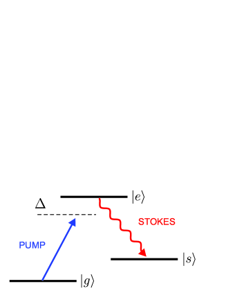
Figure 1: Atomic level configuration.

In the interaction picture, and after adiabatically eliminating the upper level $\left|e\right>$, the interaction of the light field with the atomic cloud can be described by the Hamiltonian cirac2002

$$\begin{split}H(t)=&\sum_{i=1}^{N}\hat{\sigma}_{sg}^{i}\int d{\bf k}g_{\bf k}a^{\dagger}({\bf k})\exp\left\{i\Delta\omega t\right\}u\left({\bf r}_{\perp,i}\right)\xi\left(t\right)\\ &\times\exp\left\{-i\Delta{\bf k}\cdot{\bf r}_{i}\right\}+h.c.,\end{split}$$ (3)

where $\hat{\sigma}_{sg}^{i}=\left|s\right>_{i}\left<g\right|$ is the transition operator for the ith atom, ${\bf r}_{i}=(x_{i},y_{i},z_{i})$ is the vector position of the ith atom, $g_{{\bf k}}$ is the coupling coefficient of the transition, $\Delta\omega=\omega-\left(\omega_{0}-\omega_{sg}\right)$ and $\Delta{\bf k}={\bf k}-k_{0}\hat{z}$, with $\omega_{sg}$ being the transition frequency between states $\left|g\right>$ and $\left|s\right>$.

Before the interaction, we consider that all the atoms are in the ground state and that there are no photons in the optical modes, i.e, $\left|\Psi\right>_{0}=\left|g_{1}...g_{i}...g_{N}\right>\otimes\left|0\right>_{\bf k}$. Then, considering that the pump field is weak enough, we can make use of first-order perturbation theory to write the state of the system as

$$\begin{split}\left|\Psi\right>=&\left|\Psi\right>_{0}-i\;\varepsilon\left(\Delta\omega\right)\sum_{i=1}^{N}\int d{\bf k}\;u\left({\bf r}_{\perp,i}\right)\\ &\times\exp\left\{-i\Delta{\bf k}\cdot{\bf r}_{i}\right\}\left|g_{1}...s_{i}...g_{N}\right>|{\bf k}\rangle,\end{split}$$ (4)

where $\varepsilon(\Delta\omega)=\int_{0}^{t}dt^{\prime}g\hskip 2.27621pt\xi(t^{\prime})\exp(i\Delta\omega t^{\prime})$. We assume that $\Delta{\bf k}$ becomes independent of the frequency and that $g=g_{{\bf k}}$ has the same value for all allowed directions of emission of the Stokes photons.

The use of perturbation theory is motivated by experiments in which a weak pump pulse and a short interaction time are used in order to guarantee that the probability of creating more than one excitation in the collective atomic state is very low kimble2003 ; kuzmich2005 ; kimble2005 ; inoue2006 . This weak-pumping condition makes a perturbative approach suitable for describing a realistic situation.

In the case of cold atomic ensembles, since the atoms are considered to be fixed in their positions, we can directly use Eq. (4) to obtain that the probability of emitting a photon in a given direction ${\bf k}$ is equal for all directions, i.e., there is no preferred direction of emission scully2003 ; scully2006 , independently of the specific shape of the atomic cloud, always that it is not forbidden by the transition matrix elements.

In the case of hot atomic ensembles, due to the fact that during the light-atom interaction time the atoms are moving fast, an average value over all positions ${\bf r}_{i}$ should be performed cirac2002 ; eberly2006 . The resulting state becomes

$$\begin{split}\left|\Psi\right>=&\left|\Psi\right>_{0}-i\varepsilon\left(\Delta\omega\right)\int d{\bf k}\;F\left(\Delta{\bf k}\right)|{\bf k}\rangle\otimes\sum_{i=1}^{N}\left|g_{1}...s_{i}...g_{N}\right>\end{split}$$ (5)

where the average value over all positions is expressed as $F\left(\Delta{\bf k}\right)=\int d{\bf r}u({\bf r}_{\perp})\exp\left\{-i\Delta{\bf k}\cdot{\bf r}\right\}p_{dis}({\bf r})$, with $p_{dis}({\bf r})$ being the atomic distribution function. From Eq. (5), one can show that the Stokes photons are emitted in a small cone around the forward direction (see cirac2002 for a detailed calculation), whose width depends on the particular spatial shape of the atomic cloud. Notice that, in this case, the photon and atomic degrees of freedom can be decoupled, and the quantum state of the atoms is the so-called symmetric collective atomic state, i.e., $\left|s_{a}\right>=1/\sqrt{N}\,\sum_{1}^{N}\left|g_{1}...s_{i}...g_{N}\right>$.

Equation (4) does not show any temperature dependence, so in its present form cannot be used to describe the transition between the two limiting scenarios considered so far: warm and cold atomic ensembles. In order to model the temperature dependence, we introduce a function that describes the movement of each atom around its mean position ${\bf r}_{i}$,

$$f\left({\bf r},{\bf r}_{i}\right)=\frac{1}{\pi^{3/2}A^{3}\left(T\right)}\exp\left[-\frac{\left|{\bf r}-{\bf r}_{i}\right|^{2}}{A^{2}\left(T\right)}\right],$$ (6)

where $A\left(T\right)=v_{a}\tau$ determines the radius of the area over which the atoms can move during the interaction time. It depends on the pump pulse duration ($\tau$), and on the speed ($v_{a}=\sqrt{2K_{B}T/m}$) most likely to be possessed by any atom of the system. Here $m$ is the mass of the atom, $K_{B}$ is the Boltzmann constant and $T$ is the temperature of the atomic ensemble. Notice that the origin of $v_{a}$ lies in the Maxwell$-$Boltzmann distribution. This distribution is assumed, because it has been shown that the Maxwell-Boltzmann distribution provides an accurate description of the motion of atoms at temperatures above tenths of $\mu K$ lett1988 ; lett1989 . Hence, Eq. (6) is useful for describing the motion of atoms undergoing a transition from the hot to the cold condition, provided that the lowest temperature values are above tenths of $\mu K$.

Making use of the function given in Eq. (6) to rewrite Eq. (4), the temperature-dependent quantum state of the system atoms-photon can be written as

$$\begin{split}\left|\Psi\right>=&\left|\Psi\right>_{0}-i\varepsilon\left(\Delta\omega\right)\sum_{i=1}^{N}\int d{\bf k}\int_{V}d{\bf r}f\left({\bf r},{\bf r}_{i}\right)u\left({\bf r}_{\perp}\right)\\ &\times\exp\left\{-i\Delta{\bf k}\cdot{\bf r}\right\}\left|g_{1}...s_{i}...g_{N}\right>|{\bf k}\rangle,\end{split}$$ (7)

where $V$ is the volume of the cloud.

Note that, in the limit where $A\rightarrow 0$, the function given in Eq. (6) tends to a Dirac delta function, and we recover the state of the system described by Eq. (4).

In order to obtain the angular distribution of the emitted Stokes photons, we trace out the atomic variables of the density matrix of the system ($\rho=\left|\Psi\right>\left<\Psi\right|$). Neglecting the vacuum contribution, the reduced density matrix of the photon state writes

$$\rho_{s}=\sum_{i=1}^{N}\int d{\bf k}d{\bf k}^{\prime}S({\bf r}_{i},{\bf k})S^{*}({\bf r}_{i},{\bf k^{\prime}})|{\bf k}\rangle\langle{\bf k}^{\prime}|,$$ (8)

where

$$S({\bf r}_{i},{\bf k})=\int_{V}d{\bf r}f({\bf r},{\bf r}_{i})u({\bf r}_{\perp})\exp\left(-i\Delta{\bf k}\cdot{\bf r}\right).$$ (9)

Considering that the atoms are contained in a cell with transversal dimensions $L_{x}$, $L_{y}$ and length $L_{z}$, we can solve Eq. (9) to obtain

$$S({\bf r}_{i},{\bf k})=\frac{1}{8}\alpha^{2}\Phi(x_{i},k_{x})\Phi(y_{i},k_{y})\Omega(z_{i},k_{z}),$$ (10)

where

$$\alpha = \left(\frac{r_{0}^{2}}{A^{2}+r_{0}^{2}}\right)^{1/2},$$ (11)

$$\Phi(x_{i},k_{x}) = \exp\left[-\frac{1}{4}k_{x}^{2}r_{0}^{2}-\left[\frac{\alpha}{r_{0}}\left(x_{i}+i\frac{1}{2}r_{0}^{2}k_{x}\right)\right]^{2}\right]$$ (12)

$$\times\left\{\mathrm{erf}\left[-\frac{1}{2}\alpha^{3}\left(2x_{i}-ik_{x}A^{2}-\frac{L_{x}}{\alpha^{2}}\right)\right]-\mathrm{erf}\left[-\frac{1}{2}\alpha^{3}\left(2x_{i}-ik_{x}A^{2}+\frac{L_{x}}{\alpha^{2}}\right)\right]\right\},$$

$$\Omega(z_{i},k_{z}) = \exp\left[-\frac{1}{4}k_{z}^{2}A^{2}-ik_{z}z_{j}\right]$$ (13)

$$\times\left\{\mathrm{erf}\left[-\frac{1}{2A}\left(2z_{i}-ik_{z}A^{2}-L_{z}\right)\right]-\mathrm{erf}\left[-\frac{1}{2A}\left(2z_{i}-ik_{z}A^{2}+L_{z}\right)\right]\right\}.$$

Notice that the presence of the error function (erf(x)) in Eq. (10) is due to the integration over the finite volume (V) of the cell that contains the atoms.

We now find that the probability of emitting a Stokes photon in the direction ${\bf k}$ is given by the diagonal terms of the density matrix (8),

$$P({\bf k})=\sum_{i=1}^{N}\left|S\left({\bf r}_{i},{\bf k}\right)\right|^{2},$$ (14)

where the normalization condition writes $\sum_{i=1}^{N}\int d{\bf k}\left|S\left({\bf r}_{i},{\bf k}\right)\right|^{2}=1$. In general, since the atomic cloud contains a large atom number density, the atomic summation can be rewritten as $\sum_{i=1}^{N}\rightarrow(N/V)\int dV$.

Note that Eq. (14) needs to be solved numerically due to the presence of the error function in Eq. (10). Notwithstanding, since the functions of the spatial variables are separated (as can be seen in Eq. (10)), the numerical integration of Eq. (14) can be easily performed.

III angular distribution of emitted Stokes photons

We have calculated the angular distribution of the emitted Stokes photons considering an ensemble of ⁸⁷Rb atoms contained in a pencil-shaped cell with transversal dimensions: $L_{x}=L_{y}=2$ mm, and length $L_{z}=30$ mm. The atoms are illuminated by a pump pulse with a transversal shape given by $u({\bf r}_{\perp})\sim\exp\left\{-(x^{2}+y^{2})/r_{0}^{2}\right\}$, where $r_{0}=2$ mm is the beam waist of the pump beam. The level configuration of the atoms is set to $5^{2}P_{1/2}$ for the excited level $\left|e\right>$, and the Zeeman-splitting levels $5^{2}S_{1/2}\left(F=1\right)$ and $5^{2}S_{1/2}\left(F=2\right)$ for the $\left|g\right>$ and $\left|s\right>$ states, respectively.

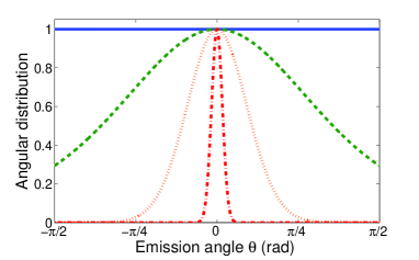
Figure 2: Angular distribution of emitted Stokes photons for different temperatures of the atomic cloud. Solid line: $T=100$ $\mu$K; Dashed line: $T=1$ K; Dotted line: $T=10$ K and Dash-dotted line: $T=300$ K. In all cases, the pump pulse duration is set to $\tau=10$ ns.

Figure 2 shows the angular distribution (normalized to the maximum) of emitted Stokes photons as a function of the angle ($\theta$) between the direction of the pump and the emitted photon (as shown in Fig. 3(a)). In the low temperature limit, the spontaneous emission of Stokes photons has no preferred direction. This result agrees with ref. kimble2003 , in which Stokes photons are said to be emitted into $4\pi$ steradian. In contrast, as the temperature of the cloud is increased, the probability distribution narrows around $\theta=0^{\circ}$, evidencing the fact that, in the case of warm atomic ensembles, Stokes photons are emitted preferentially along the direction of the pump, as it has been experimentally observed, for instance in lukin2003 .

The results shown in Fig. 2 can be understood in terms of the which-way information left in the atoms after emitting a Stokes photon, i.e., information about the position of the atom that emitted the photon. On one hand, for the case of cold atoms, due to the fact that they are fixed, one can obtain, in principle, information about the position of the atom that emitted the photon. In this situation, the possible paths of the Stokes photon will not interfere, because which-way information has been left in the atomic ensemble. This can be clearly seen from Eq. (14), which for cold atomic ensembles takes the form

$$P_{cold}({\bf k})=\sum_{i=1}^{N}\left|u\left({\bf r}_{\perp,i}\right)\right|^{2}.$$ (15)

Equation (15) shows that emission of Stokes photons from a cold atomic ensemble has no preferred direction.

On the other hand, notice that for the case of hot atomic ensembles, Eq. (6) is a constant inside the integration volume, so we can write Eq. (14), by means of the large atom number density relation, as

$$P_{hot}({\bf k})=\left|\sum_{i=1}^{N}u\left({\bf r}_{\perp,i}\right)e^{-i\Delta{\bf k}\cdot{\bf r}_{i}}\right|^{2}.$$ (16)

We see from Eq. (16) that interference between the possible paths of the Stokes photon is now restored, because which-way information has been erased by the movement of the atoms in the cloud. Interestingly, this which-way information effect has been also observed, for instance, in the context of second-order interference of single photons mandel1991 .

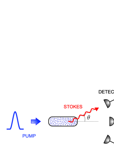
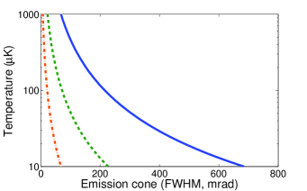
Figure 3: (a) Proposed experimental setup: an array of detectors is used to measure the width of Stokes emission cone, which allows to determine the temperature of the atomic ensemble. (b) Temperature of the atomic cloud as a function of the FWHM of the emission cone for different pulse durations. Solid line: $\tau=10$ $\mu$s; Dashed line: $\tau=30$ $\mu$s; Dash-dotted line: $\tau=100$ $\mu$s.

It is important to highlight that, it is not the actual acquisition of information from the system which determines the rise of interference, but that in principle, it would be possible to obtain such information mandel1999 .

IV experimental proposal

The close relationship between the width of the emission cone and the temperature of the atomic ensemble allows us to put forward a new technique to determine the temperature of atomic clouds. The proposed experimental setup consists of an array of detectors (or a movable detector) that would be able to detect Stokes photons along different directions, as depicted in Fig. 3(a). In this way, by measuring the width of the emission cone, we can make use of Eq. (14) to retrieve information about the temperature of the atomic ensemble. Figure 3(b) shows the temperature of the atomic ensemble as a function of the full width at half maximum (FWHM) of the emission cone. Notice that, by choosing a sufficiently short pulse, the relationship between the emission cone width and the temperature gets smoother. This can be useful for a better discrimination of the width of the emission cone, enhancing thus the precision of the technique. Also, notice that this technique is not based on the ballistic expansion of the atomic cloud lett1988 , so each measurement can be performed without destroying it.

V Heralded generation of the symmetric atomic state

We can also use Eq. (7) to describe how the generation of the symmetric state depends on the temperature of the atomic cloud. When the Stokes photon is detected in an arbitrary direction ${\bf k}$, i.e., is projected into the state $|{\bf k}\rangle$, the corresponding quantum state of the atomic cloud is

$$\left|\Psi\right>_{a}=\sum_{i=1}^{N}S\left({\bf r}_{i},{\bf k}\right)\left|g_{1}...s_{i}...g_{N}\right>.$$ (17)

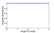
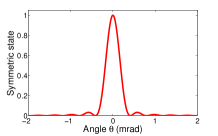
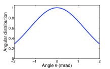
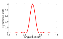
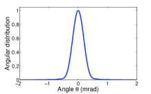
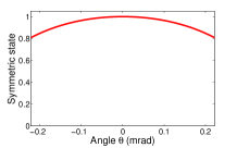
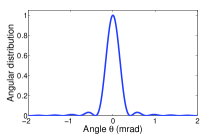
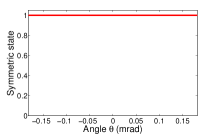
Figure 4: Angular distribution of the emitted Stokes photons ((a),(c),(e) and (g)), and the weight of the symmetric atomic state $\left|\left\langle s_{a}|\Psi\right\rangle_{a}\right|^{2}$ (within the FWHM of the emission cone) ((b), (d), (f) and (h)) for different radius of the region where the atoms are let to move: (a,b) A=1 $\mu$m, (c,d) A=100 $\mu$m, (e,f) A=1 mm, and (g,h) A=100 mm. Pulse duration: 10 $\mu$s.

In the case where the atoms are barely moving during the interaction time, only a small fraction of generated photons (those in a small angle around the pump beam direction) corresponds to the symmetric state, even though photons are emitted in a larger emission cone. This can clearly be seen by comparing Figs. 4(a) and (b), where we plot the projection $\left|\left\langle s_{a}|\Psi\right\rangle_{a}\right|^{2}$. When the atoms are let to move within the cloud by increasing the temperature, the which-way information is erased and the emission cone gets narrower (see Fig. 4(g)). In this case, as it can be seen from Fig. 4(h), photons emitted in all allowed possible directions are in the symmetric state. Notwithstanding, we are again forced to consider small emission angles around the pump beam direction to enhance the flux of detected Stokes photons. Therefore, in all cases, photons should be collected in a small cone around the direction of propagation of the pump beam, if the goal is to generate the symmetric atomic state. But as Fig. 4 shows, the reason behind this restriction depends on the temperature of the atomic ensemble.

VI conclusion

In this paper, we have presented a new technique to measure the temperature of atomic ensembles, based on the relationship between the temperature of the ensemble and the width of the emission cone of the spontaneously emitted Stokes photons. We have also shown that heralded generation of the collective symmetric atomic state requires the detection of the heralding Stokes photon in a narrow cone around the direction of the exciting pulse. For cold atomic ensembles, this is the only direction of emission that guarantees the generation of such state, while for warm ensembles, it is the direction with the highest efficiency.

- (1) L.-M. Duan, M. D. Lukin, J. I. Cirac, and P. Zoller, Nature (London) 414, 413 (2001).
- (2) L.-M. Duan, Phys. Rev. Lett. 88, 170402 (2002).
- (3) C. H. van der Wal, M. D. Eisaman, A. André, R. L. Walsworth, D. F. Phillips, A. S. Zibrov, and M. D. Lukin, Science 301, 196 (2003).
- (4) A. Kuzmich, W. P. Bowen, A. D. Boozer, A. Boca, C. W. Chou, L.-M. Duan, and H. J. Kimble, Nature (London) 423, 731 (2003).
- (5) N. Sangouard, C. Simon, H. de Riedmatten, and N. Gisin, Rev. Mod. Phys. 83, 33 (2011).
- (6) L. M. Duan, J. I. Cirac and P. Zoller, Phys. Rev. A 66, 023818 (2002).
- (7) M. O. Scully and M. S. Zubairy, Science 301, 181 (2003).
- (8) M. O. Scully, E. S. Fry, C. H. Raymond Ooi, and K. Wódkiewicz, Phys. Rev. Lett. 96, 010501 (2006).
- (9) D. N. Matsukevich, T. Chanelière, M. Bhattacharya, S.-Y. Lan, S. D. Jenkins, T. A. B. Kennedy, and A. Kuzmich, Phys. Rev. Lett. 95, 040405 (2005).
- (10) D. Felinto, C. W. Chou, H. de Riedmatten, S. V. Polyakov, and H. J. Kimble, Phys. Rev. A 72, 053809 (2005).
- (11) R. Inoue, N. Kanai, T. Yonehara, Y. Miyamoto, M. Koashi, and M. Kozuma, Phys. Rev. A 74, 053809 (2006).
- (12) P. D. Lett, R. N. Watts, C. I. Westbrook, W. D. Phillips, P. L. Gould, and H. J. Metcalf, Phys. Rev. Lett. 61, 169 (1988).
- (13) P. D. Lett, W. D. Phillips, S. L. Rolston, C. E. Tanner, R. N. Watts, and C. I. Westbrook, J. Opt. Soc. Am. B 6, 2084 (1989).
- (14) C. I. Westbrook, R. N. Watts, C. E. Tanner, S. L. Rolston, W. D. Phillips, P. D. Lett, and P. L. Gould, Phys. Rev. Lett. 65, 33 (1990).
- (15) J. Y. Courtois, G. Grynberg, B. Lounis, and P. Verkerk, Phys. Rev. Lett. 72, 3017 (1994).
- (16) M. Mitsunaga, M. Yamashita, M. Koashi, and N. Imoto, Opt. Lett. 23, 840 (1998).
- (17) J. H. Eberly, J. Phys. B: At. Mol. Opt. Phys. 39, S599 (2006).
- (18) X. Y. Zou, L. J. Wang, and L. Mandel, Phys. Rev. Lett. 67, 318 (1991).
- (19) L. Mandel, Rev. Mod. Phys. 71, S274 (1999).