Three unequal masses on a ring and soft triangular billiards

Abstract

The dynamics of three soft interacting particles on a ring is shown to correspond to the motion of one particle inside a soft triangular billiard. The dynamics inside the soft billiard depends only on the masses ratio between particles and softness ratio of the particles interaction. The transition from soft to hard interaction can be appropriately explored using potentials for which the corresponding equations of motion are well defined in the hard wall limit. Numerical examples are shown for the soft Toda-like interaction and the error function.

Hard walls in billiard systems were extensively modelled by $\delta$-potentials since they allow for simple analytical relations of velocities and angles before and after the collisions with the walls. However, equations of motion are not well defined at the collision point. To analyze the transition to soft walls, which are more realistic, it is essential to have well defined equations of motion since in general no simple analytical solutions are obtained. The present work suggests that appropriated soft walls are those for which the forces, not the potentials, become $\delta$-functions in the limit of hard walls. This allows for better numerical investigation of the soft-hard transition. A general scaled Hamiltonian is derived for three unequal masses interacting particles on a frictionless ring, which nicely describes this transition and shows that the dynamics occurs inside a soft triangle billiard.

I Introduction

Although physically realizable potentials are inherently soft, theoretical models usually focus on hard potentials since they allow for analytical solutions. Billiard systems with hard walls are one example of such theoretical models and have been extensively study and well understood. For example, it is well know Casati and Prosen (1999); Glashow and Mittag (1996); Artuso et al. (1997) that the motion of three particles on a frictionless ring with point-like interactions is equivalent to the motion of one particle moving freely inside the triangular billiard which hard walls. In such description the hard-walls potentials are represented by $\delta$-functions which makes the collisions with the walls very simple, and analytical results can be obtained for the real dynamics and also in the tangent space. However, not much has been done in the description of the transition from hard to soft interactions. Soft walls apparently do not destroy trajectories found in the hard-wall limit Rapoport et al. (2007) and induce the appearance of regular islands in phase space Turaev and Rom-Kedar (1998); Rom-Kedar and Turaev (1999); Turaev and Rom-Kedar (2003); Oliveira et al. (2008). Some works about the dynamics in soft billiard have to be mentioned, one particle motion in an atom-optic billiard Kaplan et al. (2001, 2004), quantum conductance in the soft wall microwave billiard Weingartner et al. (2005), the effect of wall roughness in granular Poiseuille flow Vijayakumar and Alam (2007) and how the confinement of the equilibrium hard-sphere fluid to restrictive one- and two-dimensional channels with soft interacting walls modifies its structure, dynamics, and entropy Mittal et al. (2006, 2007) and nonlinear dynamics in general Donnay (1999).

There is a key issue for an appropriate description of soft to hard transitions in the context of billiards. Usually the hard walls are modelled by $\delta$-functions which allow for a simple description of the collision processes, since variables (angle and velocity) before and after the collisions with the walls can be given explicitly. However, the corresponding equations of motion are not well defined. In the case of soft walls the variables before and after the collisions cannot be given in general explicitly, and equations of motion must be solved numerically. Thus, in order to study continuously the transition from soft to hard walls, equations of motions must be well defined in all cases. A first contribution Oliveira et al. (2008) in this direction analyzed the dynamics of two interacting particles inside a 1D billiard with soft walls, where the soft walls were modelled by the error function, which describes continuously and correctly the mentioned transition. The purpose of the present work is to generalize these results to the case of three soft interacting particles on a ring, and analyze the correct transition to point-like collisions. A general scaled Hamiltonian is derived which nicely describes this transition and also shows that the dynamics occurs inside a soft triangle billiard. The dynamics depends only on the masses ratio between particles and softness ratio of the interaction.

The paper is organized as follows. While in Section II the hard wall triangle billiard is revisited, Section III presents the general soft Hamiltonian system for three interacting particles, our main analytical result. In Section IV we apply the soft Hamiltonian to the Toda model with unequal masses. Section V presents the example of two suitable potential which could be used to appropriately describe the soft to hard transition for three particles. Finally Section VI summarizes our main results.

II Revisiting the hard triangular billiard

It is well know Casati and Prosen (1999); Glashow and Mittag (1996); Artuso et al. (1997) that the motion of three particles on a frictionless ring with point-like interactions is equivalent to one particle moving freely inside the triangular billiard with angles

$$\tan{\alpha}=\sqrt{\frac{m_{2}M}{m_{1}m_{3}}},\ \tan{\beta}=\sqrt{\frac{m_{1}M}{m_{2}m_{3}}},\ \tan{\eta}=\sqrt{\frac{m_{3}M}{m_{1}m_{2}}},$$

and colliding elastically with the sides of the triangle. Here $M=m_{1}+m_{2}+m_{3}$ and $m_{i}$ is the mass of the particles ($i=1,2,3$). The Hamiltonian can be written as

$$H_{B}=K_{M}+\delta(q_{2}-q_{1})+\delta(q_{3}-q_{2})+\delta(q_{1}-q_{3}+L).$$ (1)

where $K_{M}=p_{1}^{2}/2m_{1}+p_{2}^{2}/2m_{2}+p_{3}^{2}/2m_{3}$ is the mass dependent kinetic energy. The collisions occur at $q_{1}=q_{2},q_{2}=q_{3}$ and $q_{1}=q_{3}+L$ where $L$ is the circumference of the ring. The point-like collision between particles $1$ and $2$ defines one side of the triangle at $q_{1}-q_{2}=0$, and the collision of these particles with particle $3$ defines the other two sides of the same triangle. For $m_{3}\rightarrow\infty$ ($\eta=\pi/2$) we get the right triangular billiard which corresponds to the motion of two particles $m_{1}$ and $m_{2}$ moving inside the 1D box with hard walls. In this case the interaction between particles $1$ and $2$ is the point-like collision and the fixed particle $3$ plays the role of a 1D hard-wall. In such systems the Lyapunov exponent is zero Cipriani et al. (2005); Grassberger et al. (2002) and the whole dynamics can be monitored by changing the angles of the triangle billiard Casati and Prosen (1999). It was shown Beims et al. (2007) that the Yukawa interaction between particles $1$ and $2$ is enough to generate positive Lyapunov exponents. It is also worth to mention it is possible Manchein and Beims (2009) to relate the linear instability inside the triangular billiard with the Lyapunov exponents from quadratic irrational numbers, which are related to the angles of the triangle, and thus to the masses ratio.

III The soft triangular billiard

As observed in Hamiltonian (1), the collisions with the fixed hard-wall can be represented by $\delta$-potentials. However, the corresponding equations of motion are not well defined. Therefore, to describe analytically the transition to hard walls, we include soft interactions between particles which, in a given limit, are expected to describe the collisions with the hard-walls. Let us start with the Hamiltonian of the three particles on a frictionless ring given by

$$H_{B} = K_{M}+V_{12}\left(\frac{q_{2}-q_{1}}{\sigma_{12}}\right)$$ (2)

$$+ V_{23}\left(\frac{q_{3}-q_{2}}{\sigma_{23}}\right)+V_{31}\left(\frac{q_{1}-q_{3}+L}{\sigma_{31}}\right),$$

where $\sigma_{ij}$ ($i,j=1,2,3$) defines the softness of each pairwise interaction. It is assumed that the interaction potential $V_{ij}$ between the particles depends only on the relative position between them and that for $\sigma_{ij}\to 0$ a $\delta$-like function is obtained for the corresponding force, and not for the potential. In addition, bounded motion is expected below a certain energy which will be specified later. Before going into details about the appropriated potential $V_{ij}$ which could be used, we rewrite Hamiltonian (2). Using the orthogonal transformation Casati and Prosen (1999):

$$q_{1} = -\sqrt{\frac{m_{3}}{(m_{1}+m_{2})M}}x-\frac{1}{m_{1}}\sqrt{\frac{m_{1}m_{2}}{(m_{1}+m_{2})}}y+\frac{z}{\sqrt{M}},$$ (3)

$$q_{2} = -\sqrt{\frac{m_{3}}{(m_{1}+m_{2})M}}x+\frac{1}{m_{2}}\sqrt{\frac{m_{1}m_{2}}{(m_{1}+m_{2})}}y+\frac{z}{\sqrt{M}},$$ (6)

$$q_{3} = \sqrt{\frac{(m_{1}+m_{2})}{m_{3}M}}x+\frac{z}{\sqrt{M}},$$ (9)

for the three particles on a ring, and the linear transformations $x^{\prime}=\beta x$, $y^{\prime}=\beta y$, $z^{\prime}=\beta z$, $d\tau/dt=\beta=\frac{1}{\sigma_{12}\sqrt{\mu_{12}}}$, the final scaled Hamiltonian reads (without primes)

$$H_{B}=K+{V_{12}(y)}+{V_{23}(x,y)}+V_{31}(x,y),$$ (10)

where $K={p}_{x}^{2}/2+{p}_{y}^{2}/2+{p}_{z}^{2}/2$ is the mass independent kinetic energy and

$$V_{12}(y) = V_{12}\left(-y\right),$$ (11)

$$V_{23}(x,y) = V_{23}\left[\frac{\sigma_{12}}{\sigma_{23}}(ay-bx)\right],$$ (13)

$$V_{31}(x,y) = V_{31}\left[\frac{\sigma_{12}}{\sigma_{31}}(cy+bx)-\frac{L}{\sigma_{31}}\right].$$

Here $\mu_{21}=m_{1}m_{2}/(m_{1}+m_{2})=m_{2}/(1+\gamma_{21})$ is the reduced mass between particles $1$ and $2$, $\gamma_{ij}=m_{i}/m_{j}$ is the mass ratio between particles $i$ and $j$, and $a=\frac{1}{(1+\gamma_{21})}$, $b=a\sqrt{\frac{\gamma_{21}+\gamma_{31}+1}{\gamma_{32}}}$, $c=a\gamma_{21}$. Since $\beta$ scales all coordinates, they are given in terms of the smoothness of the interaction between particles $1$ and $2$ and the reduced mass $\mu_{12}$.

The Hamiltonian (10) represents one particle with scaled mass $m=1$ inside a triangular potential with three soft walls located at $y=0,y=\frac{b}{a}x$ and $y=-\frac{b}{c}x+L/\sigma_{31}$ (See Fig. 1). The smoothness of the walls will depend not only on the form of the potentials $V_{12}(y),V_{23}(x,y),V_{31}(x,y)$ and the smoothness parameters $\sigma_{12},\sigma_{23},\sigma_{31}$, but also on $a,b,c$ which depend only on the masses ratios.

Figure 1: Scaled soft triangle. Dashed line represent changes of the wall position when the softness parameter $L/\sigma_{31}$ varies.

The Hamiltonian (10) is quite interesting since some general physical situations can be observed without choosing a specific form for the interaction potentials:

(i) The $z$ dependence dissapeared due to the translational symmetry of (2). It implies the conservation of the total linear momentum.
(ii) the coupling between center of mass ($x$) and relative ($y$) coordinates appears only in the interaction potentials $V_{31}(x,y)$ and $V_{23}(x,y)$. Thus only these potentials may generate a chaotic dynamics inside the billiard. When $V_{31}=V_{23}=0$ the Hamiltonian (10) is separable and thus integrable, as expected.
(iii) Softness affects simultaneously the center of mass and relative coordinates since the ratios $\sigma_{12}/\sigma_{23},\sigma_{12}/\sigma_{31}$ multiply both variables ($x,y$). These quantities does not change the internal angles of the soft billiard.
(iv) Changes in the masses ratio will modify the parameters $a,b$ and $c$ separately, so that center of mass and relative coordinates will vary separately. Only these quantities can change the internal angles of the billiard.
(iv) Keeping the masses ratio constant, the softness inside the triangle billiard is tailored by the ratios $\sigma_{12}/\sigma_{23}$, $\sigma_{12}/\sigma_{31}$ and $L/\sigma_{31}$. The hard wall limit is obtained by making $L/\sigma_{31}\to\infty$, i. e. the wall $V_{31}$ moves to the right maintaining its inclination and the triangle size increases more and more. See dashed lines in Fig. 1.

The Hamiltonian (10) is quite general. Any interaction potential $V_{12},V_{23},V_{31}$ between particles can be used: Coulomb, Yukawa, Wood-Saxon, exponential etc. If the potential obeys the softness limits mentioned above, the properties (i)-(iv) should be valid for any of such interactions. Just to exemplify this we discuss next the well known Toda potential Toda (1970).

IV Toda potential

IV.1 Equal masses

We consider the three-particle Toda lattice Toda (1970) whose potential is obtained by using $V_{12}=e^{(q_{2}-q_{1})},V_{23}=e^{(q_{3}-q_{2})},V_{31}=e^{(q_{1}-q_{3})}$ with $L=0$ so that

$$H_{T}^{e}=K+e^{(q_{2}-q_{1})}+e^{(q_{3}-q_{2})}+e^{(q_{1}-q_{3})},$$ (15)

and corresponds to three equal masses particles moving on a ring. The letter $e$ stands for equal masses. Here the variables $q_{1},q_{2},q_{3}$ are the angles of particles related to the origin of the ring. In addition to the total energy and the linear momentum, this problem is know to have a third non-trivial integral of motion (For more details see Lichtenberg and Lieberman (1992)). Using the transformation (9) for the particular case of equal masses, the following two dimensional potential is obtained:

$$V_{T}^{e}=\left[e^{(2y+2\sqrt{3}x)}+e^{(2y-2\sqrt{3}x)}+e^{(-4y)}\right].$$ (16)

The equipotential lines for this potential look like from a soft triangle (See Fig. (1.8) from Lichtenberg and Lieberman (1992)). Therefore the analogy with the soft triangular billiard is evident. The additional isolated integral of motion is Hénon (1974):

$$I = 8p_{x}(p_{x}^{2}-3p_{y}^{2})+(p_{x}+\sqrt{3}p_{y})e^{2y-2\sqrt{3}x}$$ (19)

$$-2p_{x}e^{-4y}+(p_{x}-\sqrt{3}p_{y})e^{2y+2\sqrt{3}x},$$

which is not related to any obvious conservation law or symmetry. Potential (15) is a nice example of the soft triangular description from Eq. (10).

IV.2 Unequal masses

The unequal mass Toda problem was firstly studied numerically G.Casati and J.Ford (1975) for the case of two masses interacting in the Hamiltonian

$$H_{T}^{u}=K_{M}+e^{-q_{1}}+e^{-(q_{2}-q_{1})}+e^{q_{2}}-3,$$ (20)

where $u$ denotes unequal masses. They showed the transition to stochasticity when $m_{1}\neq m_{2}$ and confirmed the integrability for $m_{1}=m_{2}$. The three unequal masses particles was analyzed B.Dorizzi et al. (1984) for a free-end lattice Hamiltonian $H_{T}^{free}=K_{M}+e^{\epsilon(q_{1}-q_{2})}+e^{(q_{2}-q_{3})}$. They found that this problem is integrable when $m_{1}=\epsilon(2\epsilon-1)/(2-\epsilon),m_{2}=2\epsilon-1$ and $m_{3}=1$. The parameter $\epsilon$ must satisfy $1/2<\epsilon<2$. The Hamiltonian $H_{T}^{free}$ describes a scattering problem and the integrability cannot be verified numerically. Compared to the potential (15), the system $H_{T}^{free}$ does not consider the interaction bettwen particles $1$ and $3$ because it is along a lattice line. See also H.Yoshida et al. (1987) for more about the integrability of Toda kind lattices. The full problem of the Toda-like Hamiltonian with three unequal masses ($m_{1}=m_{2}=m_{3}=1$) was studied before T.Bountis et al. (1982) and has the form $H_{T}=K_{M}+e^{\delta(q_{1}-q_{2})}+e^{\epsilon(q_{2}-q_{3})}+e^{(q_{1}-q_{3})}$. Using the Painlevé property, they found the system to be integrable only for $m_{1}=m_{2}=\delta=\epsilon=1$, which is again the Toda case discussed above.

Although it is not the purpose of the present work to study the Toda potential, it can be written in the form $H=K_{M}+V_{T}^{u}$ where

$$V_{T}^{u}=e^{-\frac{1}{\sigma_{13}}(q_{1}-q_{3})}+e^{-\frac{1}{\sigma_{21}}(q_{2}-q_{1})}+e^{-\frac{1}{\sigma_{32}}(q_{3}-q_{2})},$$ (21)

which now includes the the softness parameters $\sigma_{ij}$ between each pair ($i,j$) interaction. Using Eqs. (9) in the potential (21) we obtain the two dimensional version

$$V_{T}^{u}=e^{\left(-y\right)}+e^{\left[\frac{\sigma_{12}}{\sigma_{23}}(ay-bx)\right]}+e^{\left[-\frac{\sigma_{12}}{\sigma_{13}}(cy+bx)\right]}.$$ (22)

The whole mass dependence is now inside the parameters from the potential $V_{T}^{u}$. The non trivial invariant (19) does not exist anymore for the case of unequal masses. This was checked by testing the condition $dI^{u}/dt=0$, where $I^{u}$ is the conservative quantity, similar to Eq. (19), but for the case of unequal masses.

The important point to mention here is that the integrability of the system (22) depends only on the masses ratios $m_{2}/m_{1}=m_{3}/m_{1}=m_{3}/m_{2}=1$ and the softness ratios $\sigma_{12}/\sigma_{23}=\sigma_{12}/\sigma_{13}=1$. This generalizes the result from T.Bountis et al. (1982).

In a realistic problem, like quantum dots for example, the material of the boundaries has impurities so that the interaction softness between different particles may suffer small changes. In such cases variations of the softness ratios may destroy the integrability. This can be very nicely seen in Fig. 2 where the Poincaré Surface of Section (PSS) is shown for small variations of the softness ratios. Figure 2(a) is the integrable case $m_{2}/m_{1}=m_{3}/m_{1}=m_{3}/m_{2}=1$ and $\sigma_{12}/\sigma_{23}=\sigma_{12}/\sigma_{13}=1$, while Fig. 2(b) we used $\sigma_{12}/\sigma_{23}=\sigma_{12}/\sigma_{13}=1.2$, keeping the masses ratios equal one. A change in the dynamics is observed and the chaotic motion becomes stronger.

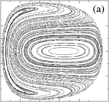
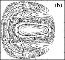
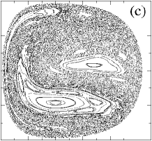
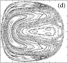
Figure 2: Poincaré Surfaces of Section ($-4.0\leq y\leq 7.0,-10\leq p_{y}\leq 10$) for $E=50$ and (a) Integrable Toda case $\gamma_{21}=\gamma_{31}=\gamma_{32}=1.0$, $\sigma_{12}/\sigma_{23}=\sigma_{12}/\sigma_{13}=1.0$, (b) small softness asymmetry $\gamma_{21}=\gamma_{31}=\gamma_{32}=1.0$, $\sigma_{12}/\sigma_{23}=\sigma_{12}/\sigma_{13}=1.2$ and the masses symmetric cases ($\sigma_{12}/\sigma_{23}=\sigma_{12}/\sigma_{13}=1.0$) (c) $\gamma_{21}=\gamma_{31}=1.2,\gamma_{32}=1.0$ and (d) $\gamma_{21}=1,\gamma_{31}=\gamma_{32}=1.2$.

It is also possible to change the masses ratio keeping the softness ratios equal one, as can be see in Fig. 2(c) and (d). Strong chaotic behavior occurs when $\gamma_{21}=\gamma_{31}=1.2,\gamma_{32}=1$, but a not that large chaotic motion for $\gamma_{21}=1,\gamma_{31}=\gamma_{32}=1.2$ in Fig. 2(d).

V Soft suitable potentials

To study the apropriate soft hard transition, in this work we assume potential functions which in limit of hard-walls are not $\delta$-functions but the corresponding forces are. In this way the potential and forces are well defined for any softness of the potential. Consider, for example, the following three potentials and the corresponding forces:

$$V_{exp}(x) = e^{-|x|/\epsilon},\qquad\qquad\quad F_{exp}(x)=\frac{1}{\epsilon}e^{-|x|/\epsilon},$$ (23)

$$V_{erf}(x) = \frac{\sqrt{\pi}}{2}Erf{\left(\frac{x}{\epsilon}\right)},\qquad\,F_{erf}(x)=\frac{1}{\epsilon}e^{-x^{2}/\epsilon^{2}},$$ (25)

$$V_{arc}(x) = -Arctan{\left(\frac{x}{\epsilon}\right)},\qquad F_{arc}(x)=-\frac{\epsilon}{x^{2}+\epsilon^{2}}.$$ (27)

In the hard wall limit $\epsilon\to 0$ the forces $F_{exp}(x),F_{erf}(x)$ and $F_{arc}(x)$ approach the well defined $\delta$-function. For example, Fig. 3 shows the (a) potential $V_{erf}(x)$ and (b) force $F_{erf}(x)$ for distinct softness values.

Figure 3: (Color online) (a) Potential $V_{erf}(x)$ and (b) force $F_{erf}(x)$ for softness values $\epsilon=0.1$ (continuous line) $\epsilon=0.05$ (dashed) and $\epsilon=0.01$ (points).

They show how the transition from soft to hard walls potentials and forces are well behaved. There are obviously other functions which in the limit $\epsilon\to 0$ behave like $\delta$-functions, but they are not appropriate for the purpose of the present work which considers billiard walls. To avoid a too long paper, we just discuss the potentials $V_{exp}(x)$ and $V_{erf}(x)$. Results for $V_{arc}(x)$ are approximately similar (not shown here) to $V_{erf}(x)$.

Applying the potentials $V_{exp}(x)$ and $V_{erf}(x)$ in the Hamiltonian (10) we obtain respectively the following systems

$$H_{B}^{exp} = K+2\left[e^{(-y)}+e^{\frac{\sigma_{12}}{\sigma_{23}}\left(ay-bx\right)}+e^{\frac{\sigma_{12}}{\sigma_{31}}\left(cy+bx-\frac{L}{\sigma_{31}}\right)}\right],$$ (28)

$$H_{B}^{erf} = K+Erf(-y)+Erf\left[\frac{\sigma_{12}}{\sigma_{23}}(ay-bx)\right]$$ (30)

$$+ Erf\left[\frac{\sigma_{12}}{\sigma_{31}}(cy+bx)-\frac{L}{\sigma_{31}}\right]+V_{0},$$ (32)

For $H_{B}^{erf}$ we added a constant potential $V_{0}=3.0$ so that both systems have the same total bounded energy $0.0\leq E_{B}\leq 2.0$. For $E_{B}>2.0$ the dynamics is unbounded.

V.1 The soft triangles

In this section we show that the potential energy from $H_{B}^{exp}$ and $H_{B}^{erf}$ have the form of a soft triangle. These potentials are shown,

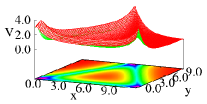
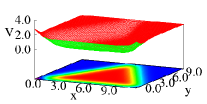
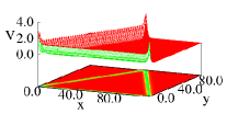
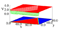
Figure 4: (Color online) Potential energy from $H_{B}^{exp}$ (left) and $H_{B}^{erf}$ (right) for the case of equal masses ratio and equal softness ratio. Top row for the soft case $L/\sigma_{31}=10$ and botton row for $L/\sigma_{31}=100$ approaching the hard-wall case.

respectively in Fig. 4 for the case of equal softness and equal masses ratio. Top row for $L/\sigma_{31}=10$ and bottom row for $L/\sigma_{31}=100$. First observation is that both potentials have a triangle billiard-like form (see projection on the $x,y$ plane) and that the walls are soft for $L/\sigma_{31}=10$. As this ratio increases to $L/\sigma_{31}=100$ the walls start to look more similar to hard-walls. For the purpose of clarity, in the left plots we used the modulus in the argument of the exponential potentials. Otherwise it would not be possible to plot the coordinates in an adequate way to see the triangle form.

For unequal masses $\gamma_{21}=5.0,\gamma_{31}=1.0$ and $\gamma_{32}=1.0/5.0$ the internal angles of the soft billiard change, as can be seen in Fig. 5, where the softness ratio are constant, and

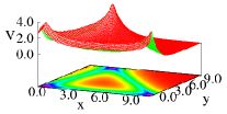
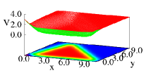
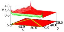
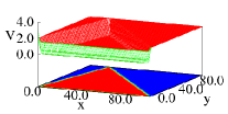
Figure 5: (Color online) Potential energy from $H_{B}^{exp}$ (left) and $H_{B}^{erf}$ (right) for the case of equal softness ratio and $\gamma_{21}=5.0,\gamma_{31}=1.0$ and $\gamma_{32}=1.0/5.0$. Top row for the soft case $L/\sigma_{31}=10$ and right bottom row for $L/\sigma_{31}=100$ approaching the hard-wall case.

top row shows results for $L/\sigma_{31}=10$ while bottom row for $L/\sigma_{31}=100$. Still we observe that $L/\sigma_{31}=100$ nicely approaches the hard-wall limit.

To make a distinction between the hard-wall case from the billiard system (1), here we say that when $L/\sigma_{31}$ increases, the quasi-hard wall limit is reached. In addition, even though we are using appropriate potentials, when $L/\sigma_{31}\gtrsim 100$ numerical difficults may appear because the potentials becomes too steep.

V.2 The dynamics

To analyze the dynamics related to the Hamiltonians from (32) we look at the PPS for the total energy $E_{B}=2.0$, which is the higher energy possible before the particle becomes unbounded.

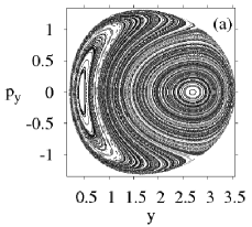
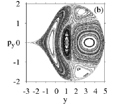
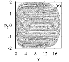
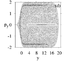
Figure 6: PSSs for $H_{B}^{exp}$ (left) and $H_{B}^{erf}$ (right) for the case of equal masses and equal softness ratio. Top PSSs are the soft case $L/\sigma_{31}=5.0$ and bottom PSSs for the quasi-hard-wall case $L/\sigma_{31}=20$.

We start showing the case of equal masses and equal softness ratios. Figure 6 compares the PSSs ($p_{y},y,p_{x}>0$) for the system $H_{B}^{exp}$ in Figs. 6(a),(c), $H_{B}^{erf}$ in Figs. 6(b),(d). The PSSs from Figs. 6(a),(b) are for the soft case $L/\sigma_{31}=5.0$, while those from Figs. 6(c),(d) for the quasi-hard-wall $L/\sigma_{31}=20$. Figures 6(a),(c) are related to the Toda potential discussed in section IV.1, but now for $L/\sigma_{31}\neq 0$. The dynamics is regular, independent of softness parameter $L/\sigma_{31}$. In this quasi-hard integrable limit trajectories travel along one invariant irrational torus (straight horizontal line) with $p_{y}>0$ ($p_{y}<0$), but when they reach the boundary with a very small softness, they invert the momentum and return along another invariant torus. The softness of the walls decide how fast this momentum inversion occurs, i.e. for quasi-hard walls the inversion occurs relatively fast [Fig. 6(c)]. For the hard wall limit from (1) it occurs instantaneously but it does not change the torus. This is valid for these integrable systems. When the dynamics from $H_{B}^{erf}$ is analyzed we see an almost regular motion in the soft walls case from Fig. 6(b). However, some hyperbolic points are present which generate a chaotic motion when $L/\sigma_{31}$ increases. This is shown in Fig. 6(d) for the quasi-hard case $L/\sigma_{31}=20$, where the motion is chaotic with two sticky motions close to $p_{y}\sim 0.0,\pm 1.7$. The sticky motion is the consequences of the periodic motion which occurs and can be clearly seen in the exponential quasi-hard limit for these points [Fig. 6(c)]. Besides these points the motion is totally chaotic. This nicely shows the numerical evidence that the integrability condition found by the original paper from Toda (1970) is only valid when an exponential function is used. Therefore, even in the quasi-hard case $L/\sigma_{31}\to\infty$ small changes in the potential interaction function may drastically change the nature of the dynamics. A chaotic motion was also observed (not shown) when the $V_{arc}(x)$ was used. It would be interesting if such integrability conditions using the exponential potentials could be applied to find another exact solutions in quantum scattering problems Luz et al. (2001); Andrade et al. (2003).

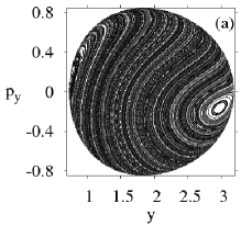
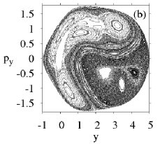
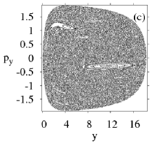
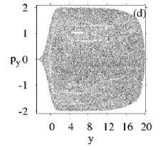
Figure 7: PSS for the case of masses ratio $\gamma_{21}=5.0,\gamma_{31}=1.0$ and $\gamma_{32}=1.0/5.0$ and equal softness ratio for $H_{B}^{exp}$ (left), $H_{B}^{erf}$ (right). Above is the soft case $L/\sigma_{31}=5$ and below the hard-wall case $L/\sigma_{31}=20$.

Figure 7 shows the dynamics when the masses ratio is changed but for equal softness ratio. The masses ratio are given by $\gamma_{21}=5.0,\gamma_{31}=1.0$ and $\gamma_{32}=1.0/5.0$. The left plots are for $H_{B}^{exp}$ and the right plots for $H_{B}^{erf}$. Figs. 7(a) and (b) are for the soft case $L/\sigma_{31}=5.0$, showing that the motion is almost regular for the exponential potential but mainly chaotic for the error potential. Figs. 7(c) and (d) are for the quasi-hard wall limit $L/\sigma_{31}=20$. In both cases the dynamics is almost chaotic.

VI Conclusions

The transition from soft to hard interaction between three particles on a frictionless ring is discussed. It is a generalization of the two soft interacting particles discussed in Oliveira et al. (2008). Since usually hard interactions are modelled by $\delta$-potentials, for which the equations of motion are not well defined, we propose suitable potentials to study the soft to hard interaction transition, where the forces, not the potentials, become $\delta$-functions in the limit of hard interactions. A scaled Hamiltonian is obtained which nicely shows this transition and gives general clues about the relevant properties of interacting particles: the dynamics depends only on the masses ratio between particles and softness ratio of the interaction, independent of the kind of interaction. Beside that any interaction potential with a parameter controlling the hard interacting limit can be used in this Hamiltonian which defines a soft triangle billiard inside which the whole dynamics occurs. The case of equal masses ratios is found to be integrable when a soft exponential interaction is assumed, like a Toda potential with a softness parameter. Equal masses ratio with other interaction potentials, like the error function and the arctan function (not shown) generate a chaotic dynamics. We consider the dynamics of two suitable potentials, the exponential interaction with an additional softness parameter, a Toda like potential, and the error function. Results show that such potentials are appropriate and they do not present numerically divergencies when approaching the hard interaction limit.