Statistical properties of spontaneous emission near a rough surface

Abstract

We study the lifetime of the excited state of an atom or molecule near a plane surface with a given random surface roughness. In particular, we discuss the impact of the scattering of surface modes within the rough surface. Our study is completed by considering the lateral correlation length of the decay rate and the variance discussing its relation to the $C_{0}$ correlation.

I Introduction

The spontaneous decay rate of an excited atom or molecule is known to depend on its environment. This effect is similar to Purcell’s effect which has been studied theoretically and experimentally in numerous works since the pioneering works by Purcell and Drexhage Purcell1946 ; DrexhageEtAl1968 . In the very close proximity of a surface the decay rate increases drastically, since the excited atom or molecule can couple to non-radiative modes. This can be related to the increase of the local density of states (LDOS) near a surface which is due to evanescent modes providing more channels into which the excited atom or molecule can decay FordWeber1984 ; Barnes1998 .

Recently, this effect which allows for controlling the decay rate of atoms and molecules has been intensively investigated for random or disordered media. In such materials the multiple scattering of electromagnetic modes results in the formation of speckles, i.e., spatial fluctuations of the LDOS. Then the spontaneous decay rate of atoms or molecules close or within such systems becomes a statistical quantity, which depends on the one hand on the local near-field environment of the source and on the other hand on the mesoscopic fluctuations of the random material itself. In particular, the fluorescence rate statistics or fluctuations of the LDOS in such media has been considered theoretically Shapiro1986 ; Shapiro1999 ; VanTiggelen2006 ; CazeEtAl2010 ; FroufeEtAl2007 and experimentally RuijgrokEtAl2010 ; BirowosutoEtAl2010 ; SapienzaEtAl2011 ; Krachmalnicoff2010 .

A random rough surface is similar to a bulk disordered medium in the sense that above such a surface the LDOS shows a spatial speckle pattern GreffetCarminati1995 . The lifetime of an atom or molecule becomes a random quantity which depends on the local environment of the particle and the statistical properties of the surface. Recently, the speckle pattern above random media Apostol2003 ; Apostol2003b ; Carminati2009 has been studied. The goal of this work is to reconsider the impact of surface roughness on the spontaneous decay rate. Previous studies have considered the impact of the surface roughness on the average decay rate for atoms or molecules near metal surfaces Arya1982 ; Aravind1980 ; AriasEtAl1981 ; Xiao1989 . Here, we will focus on the lateral correlation of the decay rates, i.e., the correlation between the decay rates of an atom or molecule placed at different positions above the rough surface by keeping the distance to the mean surface constant, and its variance. In addition, we will specifically consider the influence of surface modes for which the enhancement of the decay rate is very large.

For pedagogical reasons we consider a semi-infinite SiC material with a rough surface. Firstly, we do not have to consider nonlocal effects for the considered atom-surface distances which can be quite important for metal surfaces FordWeber1984 ; Sipe1979 ; PerssonLang1982 ; Avouris1983 ; BalzerEtAl1997 . Secondly, SiC has only one well established surface resonance and is well described by a simple model BohrenHuffman for its permittivity. Nonetheless, the results we obtain are applicable to arbitrary local, homogeneous and isotropic materials. For the description of the surface roughness we use the perturbation theory introduced in Ref. Greffet1988 up to second order within the surface profile function.

The paper is organized as follows: In Sec. 2 we give a short introduction to the calculation of decay rates close to a plane surface in the weak coupling limit. The effect of the surface roughness on the mean decay rate is discussed in Sec. 3 where we also give some interpretation of the observed roughness correction. Finally in Sec. 4 we investigate the lateral correlation and the fluctuations of the decay rate. We finish with the conclusion in Sec. 5.

II Spontaneous decay rate

For an electric-dipole transition in the weak-coupling regime, the normalized spontaneous decay rate of an atom or molecule placed at $\mathbf{r}_{\rm A}$ can be expressed as NovotnyHecht2006

$$\frac{\Gamma_{i}}{\Gamma_{\infty}}=\frac{6\pi}{k_{0}}{\rm Im}\biggl{[}\mathbf{e}_{i}^{\rm t}\cdot\mathds{G}(\mathbf{r}_{\rm A},\mathbf{r}_{\rm A},\omega_{0})\cdot\mathbf{e}_{i}\biggr{]}$$ (1)

where $\mathbf{e}_{i}$ is the unit vector in the direction of the dipole transition, ${\rm t}$ symbolizes the transposed vector, $k_{0}=\omega_{0}/c$ with $\omega_{0}$ the frequency of the dipole transition. $\Gamma_{\infty}$ is the decay rate in free space (see for example in Ref. NovotnyHecht2006 ). $\mathds{G}$ is the classical electric Green’s dyadic for the geometry considered. In our case, this geometry consists of a half-space of a given material characterized by its permittivity $\epsilon(\omega)$ with a rough surface as depicted in Fig. (1).

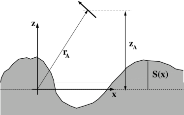
Figure 1: Sketch of a dipole at $\mathbf{r}_{\rm A}$ in a distance $z_{\rm A}$ above the mean of a rough surface described by a profile function $S$.

Before considering the role of surface roughness, we summarize the known results for a flat surface. We can derive the decay rate from Eq. (1) for a dipole moment parallel $\Gamma_{\parallel}$ and perpendicular $\Gamma_{\perp}$ to the surface by inserting the Green’s dyadic from Eq. (34) in appendix A. We find the well-known relations NovotnyHecht2006

$$\frac{\Gamma_{\parallel}^{(0)}}{\Gamma_{\infty}} =\frac{3}{4}\int_{0}^{k_{0}}\!\!\frac{{\rm d}\kappa}{k_{0}}\,\frac{\kappa}{\gamma_{\rm r}}\biggl{\{}1+{\rm Re}\bigl{(}r_{\rm s}{\rm e}^{2{\rm i}\gamma_{\rm r}z_{\rm A}}\bigr{)}+\frac{\gamma_{\rm r}^{2}}{k_{0}^{2}}\bigl{[}1-{\rm Re}\bigl{(}r_{\rm p}{\rm e}^{2{\rm i}\gamma_{\rm r}z_{\rm A}}\bigr{)}\bigr{]}\biggr{\}}$$

$$\quad+\frac{3}{4}\int_{k_{0}}^{\infty}\!\!\frac{{\rm d}\kappa}{k_{0}}\,\frac{\kappa}{\gamma}{\rm e}^{-2\gamma z_{\rm A}}\biggl{\{}{\rm Im}(r_{\rm s})+{\rm Im}(r_{\rm p})\frac{\gamma^{2}}{k_{0}^{2}}\biggr{\}},$$ (2)

$$\frac{\Gamma_{\perp}^{(0)}}{\Gamma_{\infty}} =\frac{3}{2}\int_{0}^{k_{0}}\!\!\frac{{\rm d}\kappa}{k_{0}}\,\frac{\kappa^{3}}{\gamma_{\rm r}k_{0}^{2}}\biggl{\{}1+{\rm Re}\bigl{(}r_{\rm p}{\rm e}^{2{\rm i}\gamma_{\rm r}z_{\rm A}}\bigr{)}\biggr{\}}+\frac{3}{2}\int_{k_{0}}^{\infty}\!\!\frac{{\rm d}\kappa}{k_{0}}\,\frac{\kappa^{3}}{\gamma k_{0}^{2}}{\rm e}^{-2\gamma z_{\rm A}}{\rm Im}(r_{\rm p}).$$ (3)

Here, we have introduced the lateral wave vector $\boldsymbol{\kappa}=(k_{x},k_{y})^{\rm t}$, the perpendicular wave vector $\gamma_{r}=\sqrt{k_{0}^{2}-\kappa^{2}}$ and $\gamma=\sqrt{\kappa^{2}-k_{0}^{2}}$; $r_{\rm s}$ and $r_{\rm p}$ are Fresnel’s coefficient for s- and p-polarized light. Additionally, we have split the decay rate into its radiative ($\kappa<k_{0}$) and non-radiative ($\kappa>k_{0}$) part.

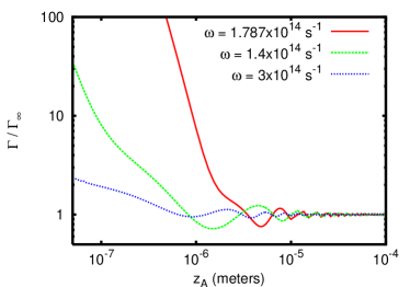
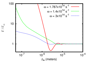
Figure 2: (Color online) Normalized decay rate of an atom in a distance $z_{\rm A}$ above a flat surface with its dipole moment oriented (left) parallel and (right) perpendicular to the surface. We have chosen the material properties of SiC at the transition frequencies $\omega_{0}=1.4\cdot 10^{14}\,{\rm s}^{-1},1.787\cdot 10^{14}\,{\rm s}^{-1}$ and $3\cdot 10^{14}\,{\rm s}^{-1}$.

In Fig. 2 we show a plot of the distance dependence of the decay rates $\Gamma_{\parallel}$ and $\Gamma_{\perp}$ for an atom near a flat SiC interface. We consider a transition frequency coinciding with the SiC surface phonon resonance at $\omega_{\omega_{\rm SPhP}}=1.787\cdot 10^{14}\,{\rm s}^{-1}$ and a transition frequency slightly smaller and slightly larger than $\omega_{\rm SPhP}$. In all three cases one finds the known characteristics of the decay rate near a flat surface Barnes1998 : i) For relative large distances $z_{\rm A}>\lambda_{0}=2\pi c/\omega_{0}$ the decay rate oscillates due to the phase change of the reflected field. ii) In the near-field regime with $z_{\rm A}<\lambda_{0}=2\pi c/\omega_{0}$ the decay rate is highly increased due to the decay into nonradiative or evanescent channels. For $\omega=1.4\cdot 10^{14}\,{\rm s}^{-1}$ and $\omega=3\cdot 10^{14}\,{\rm s}^{-1}$ the atom or molecule can decay into total internal reflection modes, whereas for $\omega=1.787\cdot 10^{14}\,{\rm s}^{-1}$ it can decay into surface phonon polaritons. It can be expected that within this near-field regime, the decay rate will be very sensitive to the multiple scattering of surface waves within a rough surface for $\omega=1.787\cdot 10^{14}\,{\rm s}^{-1}$. iii) Finally, for a distance $z_{\rm A}$ smaller than about $100\,{\rm nm}$ the decay rate diverges as $z_{\rm A}^{-3}$. This so-called quenching effect emerges from the $1/z^{3}$ electrostatic interaction of the atom’s dipole field with the surface. Therefore, this effect is extremely localized so that in this extreme near-field regime the decay rate will only be sensitive to the change of the local environment of the atom or molecule as for example to the local change of the surface geometry due to roughness.

III Roughness correction to the decay rate

Now, we turn to the effect of surface roughness on the decay rate. To this end, we consider a stochastic surface profile function $S$ describing the deviation of the rough surface from flatness (see Fig. 1). The function $S$ is modeled as a stochastic Gaussian process with mean value and correlation function given by

$$\langle S(\mathbf{x})\rangle =0,$$ (4)

$$\langle S(\mathbf{x})S(\mathbf{x}^{\prime})\rangle =\delta^{2}{\rm e}^{-\frac{|\mathbf{x-x^{\prime}}|^{2}}{a^{2}}}=\delta^{2}W(|\mathbf{x-x^{\prime}}|),$$ (5)

$\mathbf{x}=(x,y)^{t}$. The brackets $\langle\rangle$ stand for the average over an ensemble of realizations of the surface profile $S(\mathbf{x})$; $\delta$ is the rms height and $a$ the correlation length of the surface profile. It follows that the Fourier components $\tilde{S}(\boldsymbol{\kappa})$ of the surface profile function fulfill the relations

$$\langle\tilde{S}(\boldsymbol{\kappa})\rangle =0,$$ (6)

$$\langle\tilde{S}(\boldsymbol{\kappa})\tilde{S}(\boldsymbol{\kappa}^{\prime})\rangle =(2\pi)^{2}\delta^{2}\delta(\boldsymbol{\kappa}+\boldsymbol{\kappa}^{\prime})g(\kappa),$$ (7)

where we have introduced the surface roughness power spectrum

$$g(\kappa)=\int\!\!{\rm d}^{2}x\,W(|\mathbf{x}|){\rm e}^{-{\rm i}\boldsymbol{\kappa}\cdot\mathbf{x}}.$$ (8)

In the following calculations we will assume a gaussian correlation function $W(|\mathbf{x-x^{\prime}}|)=\exp(|\mathbf{x-x^{\prime}}|^{2}/a^{2})$ so that in this case $g(\kappa)=\pi a^{2}{\rm e}^{-\frac{\kappa^{2}a^{2}}{4}}$. By introducing a stochastic surface profile, the fields are scattered by that surface and hence the decay rate becomes a stochastic processes. The reflected fields can be described by a stochastic reflection coefficient which determines the decay rate in Eqs. (2) and (3). The statistics of the decay rate is itself determined by its mean value and higher moments. Here, we will concentrate on the mean decay rate and in the next section we will turn to the correlation function and the variance. By virtue of Eqs. (2) and (3) the mean decay rate depends on the mean reflection coefficients of the surface. The average restores the translational invariance so that the decay rate depends only on the distance to the surface $z_{A}$. The mean reflection coefficients can be determined perturbatively if the surface roughness is much smaller than the wavelength $\lambda_{0}$. It has been shown in Ref. BiehsGreffet that by using the perturbation theory of Ref. Greffet1988 , the correction to the Fresnel reflection coefficient $\Delta r_{{\rm s}/{\rm p}}=\langle r_{{\rm s}/{\rm p}}\rangle-r_{{\rm s}/{\rm p}}$ due to roughness is up to second-order in the surface profile given as

$$\Delta r_{{\rm s}/{\rm p}}=-2{\rm i}\gamma_{\rm r}(D_{{\rm s}/{\rm p}})^{2}M_{{\rm s}/{\rm p}}$$ (9)

where

$$D_{\rm s}=\frac{{\rm i}}{\gamma_{\rm r}+\gamma_{\rm t}}\quad\text{and}\quad D_{\rm p}=\frac{{\rm i}\epsilon}{\gamma_{\rm r}\epsilon+\gamma_{\rm t}}$$ (10)

using $\gamma_{\rm t}=\sqrt{k_{0}^{2}\epsilon-\kappa^{2}}$. The expressions for $M_{\rm s}$ and $M_{\rm p}$ can be found in Ref. BiehsGreffet . Therefore, one can easily get the second-order correction to the decay rates

$$\Delta\Gamma_{\parallel/\perp}=\frac{\langle\Gamma_{\parallel/\perp}\rangle-\Gamma_{\parallel/\perp}^{(0)}}{\Gamma_{\infty}}$$ (11)

by replacing the reflection coefficient in Eqs. (2) and (3) by $\Delta r_{{\rm s}}$ and $\Delta r_{{\rm p}}$. Now, we use the approximation for the correction to the reflection coefficient from Ref. BiehsGreffet

$$\Delta r_{{\rm s}/{\rm p}}\approx r_{{\rm s}/{\rm p}}2\kappa^{2}\delta^{2}$$ (12)

which holds in the quasi-static regime for $\kappa\gg k_{0}$ and $\kappa a\gg 1$. Since this is in the quasi-static regime equivalent to distances $z_{\rm A}\ll a$, we can conclude that for $z_{\rm A}\ll a$ we have

$$\Delta\Gamma_{\parallel/\perp}\approx 6\frac{\delta^{2}}{z^{2}_{\rm A}}\Gamma_{\parallel/\perp}^{(0)}.$$ (13)

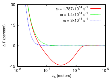
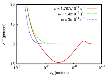
Figure 3: (Color online) Correction to the decay rate $\Delta\Gamma$ for an atom with its dipole moment oriented (left) parallel and (right) perpendicular to the mean surface. The parameters are the same as in Fig. 2. For the rough surface we choose $\delta=5\,{\rm nm}$ and $a=200\,{\rm nm}$.

In order to illustrate the effect of roughness we plot in Fig. 3 the roughness correction $\Delta\Gamma_{\parallel/\perp}$ for the same frequencies as in Fig. 2 considering a rough surface with an rms $\delta=5\,{\rm nm}$ and a correlation length $a=200\,{\rm nm}$. It can be seen that the roughness correction is very small in the large distance regime for $z_{\rm A}>\lambda_{0}$, but can be relatively large for small distances, i.e., for $z_{\rm A}<\lambda_{0}$ where the decay rate is very large due to the decay into non-radiative channels. As will be discussed in more detail in the following, electrostatic effects in the extreme near-field for $z_{\rm A}<100\,{\rm nm}$ and surface phonon polaritons in the intermediate distance regime are responsible for this relatively large correction. The first is a local effect, whereas the latter is a multiple scattering effect.

In the intermediate distance regime $100-1000$nm it can be seen on Fig. 3 that the roughness correction is slightly positive at a distance of $\approx 1000$ nm when total internal reflection modes are excited (i.e., for $\omega_{0}=1.4\cdot 10^{14}\,{\rm s}^{-1}$ and $\omega_{0}=3\cdot 10^{14}\,{\rm s}^{-1}$). For a frequency $\omega_{0}=\omega_{\rm SPhP}$ surface phonon polaritons are excited in this distance regime. Surprisingly, the presence of roughness leads to a large negative correction indicating that the lifetime is increased. This effect has been studied in Ref. BiehsGreffet in terms of the LDOS (see Fig. $14$ Ref. BiehsGreffet ) and is due to the roughness induced multiple scattering of surface modes. The scattering causes a broadening of the dispersion relation Raether . Due to this broadening as illustrated in Fig. 4 the LDOS (which is proportional to ${\rm Im}(r_{p})$) becomes smaller for frequencies close to $\omega_{\rm SPhP}$ for intermediate $\kappa$ or distances $z_{\rm A}$, respectively, explaining the observed decrease of the decay rate.

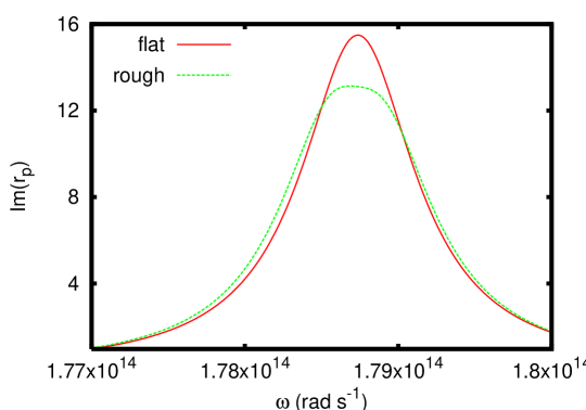
Figure 4: (Color online) Plot of ${\rm Im}(r_{p})$ for the flat and ${\rm Im}(\langle r_{p}\rangle)$ for the rough surface for $\kappa=3.3\cdot 10^{6}\,{\rm m}^{-1}$ which corresponds approximately to a distance of $z_{\rm A}\approx\kappa^{-1}=3\cdot 10^{-7}\,{\rm m}^{-1}$.

We now consider the very small distances $z_{\rm A}\ll a$ regime. The roughness correction is in this case due to the local electrostatic interaction (quenching) of the atom dipole moment with the rough surface resulting in a positive and large roughness correction to the decay rate. This quenching effect is similar for all transition frequencies as can be seen in Fig. 3. This correction can be described by the quasi-static expression in Eq. (13). We will now see that we can retrieve this expression in Eq. (13) using a simple physical argument. If $z_{\rm A}\ll a$, curvature effects are negligible so that the atom feels only the local deviation of the surface from flatness. This effect can be described by the ansatz:

$$\langle\Gamma_{\parallel/\perp}\rangle\approx\langle\Gamma(d+S(\mathbf{x}))\rangle.$$ (14)

This means that one replaces locally the surface profile by a shifted flat surface. Employing this approximation in Eqs. (2) and (3) we see that it is equivalent to the replacement of the mean reflection coefficient by

$$\langle r_{{\rm s}/{\rm p}}\rangle=r_{{\rm s}/{\rm p}}\langle e^{2{\rm i}\gamma_{\rm r}S(\mathbf{x})}\rangle.$$ (15)

Note, that this is the expression for the propagating ($\kappa<k_{0}$) and the evanescent ($\kappa>k_{0}$) part. Now, this expression can be easily evaluated, since we have assumed that $S(\mathbf{x})$ is Gaussian distributed. We find

$$\langle r_{{\rm s}/{\rm p}}\rangle=r_{{\rm s}/{\rm p}}e^{-2\gamma_{\rm r}^{2}\delta^{2}}.$$ (16)

For propagating waves such that $\kappa<k_{0}$, this is the well-known result of the Kirchhoff approximation DeSanto which holds if $\lambda\ll a$. But for $\kappa\gg k_{0}$, this approximation produces the result in Eq. (12) when expanding the exponential up to second order in the rms $\delta$. Hence, we have retrieved Eq. (13).

IV Statistical properties of spontaneous emission

We now examine the fluctuations and the spatial correlations of the decay rate above a random rough surface. The statistical properties of fields in random media has received a lot of attention in the past thirty years. Here, we are interested in some recent results relevant for our system. It has been shown recently that the intensity correlations above random media or materials with rough surfaces become non universal in the near field, i.e., they highly depend on the properties of the random media or rough surfaces GreffetCarminati1995 ; EmilianiEtAl2003 ; Apostol2003 ; Apostol2003b ; LaverdantEtAl2008 ; Carminati2010 . A remarkable connection has been established between the LDOS fluctuations and the $C_{0}$ correlation Shapiro1999 ; VanTiggelen2006 for multiple scattering media. The $C_{0}$ correlation is defined as the infinite range contribution to the correlation of the intensity in multiple scattering media Shapiro1999 . A simple explanation has been reported recently CazeEtAl2010 . Finally, the multiple scattering of surface modes in a random media or rough surface can lead to localized surface modes BozhevolnyiEtAl1995 ; BozhevolnyiEtAl1996 which show a characteristic long tail distribution of the intensity enhancement of the fields close to the surface BozhevolnyiCoello2001 ; BuilEtAl2006 . This effect can be neglected for surfaces with small roughnesses as shown for fractal surfaces SanchezGil2000 ; SanchezGil2001 . Here, we focus on the lateral correlation and the variance of the decay rate above a rough surface and we will discuss the relation of the variance to the LDOS fluctuations and $C_{0}$ correlation. Since the perturbative approach is restricted to small surface roughnesses, we will leave the problem of localization and its relation to the distribution of decay rates for future studies.

IV.1 Variance and correlation function

Before evaluating the correlation function of the decay rate, we first determine the variance which is up to second order in the surface profile given by

$$\sigma^{2}_{i}=\langle\Gamma^{2}_{i}\rangle-\langle\Gamma_{i}\rangle^{2}=\langle\Gamma^{(1)}_{i}\Gamma^{(1)}_{i}\rangle.$$ (17)

Obviously the variance is a special case of the more general correlation function

$$\langle\Gamma_{i}(\mathbf{r})\Gamma_{j}(\mathbf{r}^{\prime})\rangle=\langle\Gamma_{i}\Gamma_{j}^{\prime}\rangle_{\rm spec}+\langle\Gamma_{i}\Gamma_{j}^{\prime}\rangle_{\rm diff},$$ (18)

which can be divided into a specular (depending only on the mean field) and a diffuse contribution (due to the fluctuating part of the field). By inserting the perturbation expansion $\Gamma_{i}\approx\Gamma_{i}^{(0)}+\Gamma_{i}^{(1)}+\Gamma_{i}^{(2)}$ we find up to second order for both of these contributions

$$\begin{split}\langle\Gamma_{i}\Gamma_{j}^{\prime}\rangle_{\rm spec}&=\Gamma_{i}^{(0)}(z)\Gamma_{j}^{(0)}(z^{\prime})+\Gamma_{i}^{(0)}(z)\langle\Gamma_{j}^{(2)}(z^{\prime})\rangle\\ &\qquad+\langle\Gamma_{i}^{(2)}(z)\rangle\Gamma_{j}^{(0)}(z^{\prime})\end{split}$$ (19)

and

$$\langle\Gamma_{i}\Gamma_{j}^{\prime}\rangle_{\rm diff}=\langle\Gamma_{i}^{(1)}(\mathbf{r})\Gamma_{j}^{(1)}(\mathbf{r}^{\prime})\rangle.$$ (20)

Obviously, the specular part only depends on $z$ and $z^{\prime}$. This is due to the fact that for the mean field the translational symmetry with respect to the $x$-$y$ plane is restored after averaging, whereas for a fixed $z$ and $z^{\prime}$ the diffuse part contains lateral correlations with respect to $|\mathbf{x}-\mathbf{x}^{\prime}|$. Furthermore, we note that the variance depends on the diffuse part of the correlation function, only.

IV.2 Lateral Correlation

Now, we focus on the lateral correlation only. Therefore, we assume $z=z^{\prime}=z_{\rm A}$. The correlation function is then given by

$$\langle\Gamma_{i}(\mathbf{x})\Gamma_{j}(\mathbf{x}^{\prime})\rangle=\langle\Gamma_{i}\Gamma_{j}\rangle_{\rm spec}+\langle\Gamma_{i}(\mathbf{x})\Gamma_{j}(\mathbf{x}^{\prime})\rangle_{\rm diff}.$$ (21)

It is clear from Eq. (19) that the specular contribution is just a constant term giving an infinite range correlation depending on the distance $z_{\rm A}$ only. On the other hand, the diffuse part depends on $|\mathbf{x}-\mathbf{x}^{\prime}|$ and therefore contains the lateral short range correlations. We derive the explicit expression for the diffuse part of the correlation function in appendix C. The result can be stated as [see Eq. (54)]

$$\frac{\bigl{\langle}\Gamma^{(1)}_{i}(\mathbf{x})\Gamma^{(1)}_{j}(\mathbf{x}^{\prime})\bigr{\rangle}}{\Gamma_{\infty}^{2}}=\frac{(3\pi)^{2}}{k_{0}^{2}}2{\rm Re}\int\!\!\frac{{\rm d}^{2}\xi}{(2\pi)^{2}}\delta^{2}g(|\boldsymbol{\xi}|)F_{j}(\boldsymbol{\xi};z_{\rm A})G_{i}(\boldsymbol{\xi};z_{\rm A}){\rm e}^{{\rm i}\boldsymbol{\xi}\cdot(\mathbf{x}-\mathbf{x}^{\prime})}$$ (22)

where the functions $G_{i}$ and $F_{j}$ are defined in Eq. (55) and (56). In the following we will discuss this expression in more detail.

Let us focus on the evanescent regime, i.e., $z_{\rm A}\ll\lambda$. Then the exponential function $\exp({\rm i}\gamma_{\rm r}^{\prime}z_{\rm A})\approx\exp(-|\boldsymbol{\kappa}\pm\boldsymbol{\xi}|z_{\rm A})$ in the integrand $a_{i}$ of $F_{j}$ and $G_{i}$ [see Eq. (50)] acts as a low pass filter and restricts the contributing $\xi$ to $\xi<1/z_{\rm A}$. On the other hand, for a Gaussian roughness correlation the roughness power spectrum $g(|\xi|)$ also acts as a low pass filter restricting the $\xi$ to $\xi<1/a$. Therefore we can make simple approximations for Eq. (22) in the two limits $a\gg z_{\rm A}$ and $a\ll z_{\rm A}$.

In the case $a\gg z_{\rm A}$ the functions $F_{j}$ and $G_{i}$ can be approximated by $F_{j}(\mathbf{0};z_{\rm A})$ and $G_{i}(\mathbf{0};z_{\rm A})$. It follows immediately from Eq. (54)

$$\frac{\bigl{\langle}\Gamma^{(1)}_{i}{\Gamma^{(1)}_{j}}^{\prime}\bigr{\rangle}}{\Gamma_{\infty}^{2}}\approx(3\pi)^{2}4{\rm Im}[G_{j}(\mathbf{0};z_{\rm A})]{\rm Im}[G_{i}(\mathbf{0};z_{\rm A})]\frac{\delta^{2}}{k_{0}^{2}}W(|\mathbf{x}-\mathbf{x}^{\prime}|).$$ (23)

We can conclude from this expression that the lateral correlation function reproduces the correlation function of the surface roughness for distances such that $z_{\rm A}\ll a$, which also holds for $z_{\rm A}>\lambda$. In particular the correlation length of the lifetime correlations coincides with $a$. This means that in this distance regime one can directly measure the correlation of surface roughness by measuring the correlations of lifetimes above the surface. In the quasi-static limit the correlation function can be further simplified (see appendix D for a detailed calculation). We find

$$\frac{\langle\Gamma_{\parallel/\perp}\Gamma_{\parallel/\perp}\rangle_{\rm diff}}{\Gamma_{\parallel/\perp}^{(0)}(z_{\rm A})\Gamma_{\parallel/\perp}^{(0)}(z_{\rm A})}\approx 9\frac{\delta^{2}}{z^{2}_{\rm A}}W(|\mathbf{x-x^{\prime}}|).$$ (24)

Now, in the opposite limit, where we have $a\ll z_{\rm A}$ the roughness power spectrum $g(|\xi|)$ in Eq. (8) can be approximated by $g(0)=\pi a^{2}$ and can be taken out of the integral. The remaining expression can be further simplified in the evanescent regime assuming that the most important contributions stem from $\xi\gg k_{0}$ and $\xi\gg k_{0}|\epsilon|$. The resulting expression for the $\Gamma_{\parallel}$ can be written as (see Eq. (73) appendix D)

$$\bigl{\langle}\Gamma^{(1)}_{\perp}(\mathbf{r})\Gamma^{(1)}_{\perp}(\mathbf{r}^{\prime})\bigr{\rangle}\propto\delta^{2}a^{2}\frac{P_{3}\biggl{(}\frac{z_{\rm A}}{\sqrt{z^{2}_{\rm A}+(|\mathbf{x-x^{\prime}}|^{2}}}\biggr{)}}{[z^{2}_{\rm A}+|\mathbf{x-x^{\prime}}|^{2}]^{2}},$$ (25)

where $P_{3}$ is the Legendre polynomial of third power. Hence, for distances such that $a\ll z_{\rm A}\ll\lambda$ the lateral correlation goes rapidly to zero for $|\mathbf{x-x^{\prime}}|\gg z_{\rm A}$. Surprisingly, the lateral correlation length only depends on $z_{\rm A}$ and does neither depend on the correlation length of the surface roughness nor on the properties of the material. For $\bigl{\langle}\Gamma^{(1)}_{\parallel}(\mathbf{x})\Gamma^{(1)}_{\parallel}(\mathbf{x}^{\prime})\bigr{\rangle}$ we find a somewhat more complicated but similar expression in Eq. (74) which leads to the same conclusions. We note that a similar result was found for the intensity correlation in the near-field of a random medium Apostol2003 ; Carminati2010

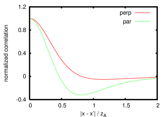
Figure 5: (Color online) Plot of the correlation functions $\bigl{\langle}\Gamma^{(1)}_{\perp}(\mathbf{r})\Gamma^{(1)}_{\perp}(\mathbf{r}^{\prime})\bigr{\rangle}$ and $\bigl{\langle}\Gamma^{(1)}_{\parallel}(\mathbf{r})\Gamma^{(1)}_{\parallel}(\mathbf{r}^{\prime})\bigr{\rangle}$ in Eq. (25) and (74) over the lateral distance $(\mathbf{x}-\mathbf{x}^{\prime})/z_{\rm A}$ normalized to their value at $\mathbf{x}=\mathbf{x}^{\prime}$.

In Fig. 5 we plot the quasistatic results of $\bigl{\langle}\Gamma^{(1)}_{\perp}(\mathbf{x})\Gamma^{(1)}_{\perp}(\mathbf{x}^{\prime})\bigr{\rangle}$ and $\bigl{\langle}\Gamma^{(1)}_{\parallel}(\mathbf{x})\Gamma^{(1)}_{\parallel}(\mathbf{x}^{\prime})\bigr{\rangle}$ from Eq. (73) and (74) for a fixed distance $z_{\rm A}$ which is assumed to be so small that the conditions for the quasistatic approximations are met, but $z_{\rm A}\gg a$. Note that the regime where these approximations are valid might be hard to achieve in practice, since the non-retarded regime starts for SiC for example for $z_{\rm A}<200\,{\rm nm}$, i.e., for distances which are not much larger than typical surface roughness correlation lengths. Nonetheless, one can expect that, for intermediate region, the correlation length is the atom-surface distance $z_{\rm A}$. To illustrate this fact, we plot in Fig. 6 numerical results for the correlation function in Eq. (23). It can be seen that for intermediate distances $a<z_{\rm A}<\lambda$ the correlation length is about $z_{\rm A}$.

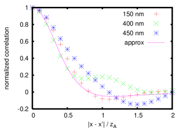
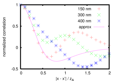
Figure 6: (Color online) Plot of the correlation functions (left) $\bigl{\langle}\Gamma^{(1)}_{\perp}(\mathbf{r})\Gamma^{(1)}_{\perp}(\mathbf{r}^{\prime})\bigr{\rangle}$ and (right) $\bigl{\langle}\Gamma^{(1)}_{\parallel}(\mathbf{r})\Gamma^{(1)}_{\parallel}(\mathbf{r}^{\prime})\bigr{\rangle}$ in Eq. (23) for different distances $z$ at $\omega_{0}=1.787\cdot 10^{14}\,{\rm s}^{-1}$ choosing the surface roughness parameters $\delta=5\,{\rm nm}$ and $a=50\,{\rm nm}$ (74). The correlation functions are normalized to their value at $\mathbf{x}=\mathbf{x}^{\prime}$. Furthermore we plot again the approximations shown in Fig. 5.

IV.3 Variance and standard deviation

Let us now return to the variance given by Eq. (17). In the quasistatic limit using Eq. (24) we find for $z\ll a$ the simple expression

$$\frac{\sigma^{2}_{\parallel/\perp}}{\biggl{[}\Gamma_{\parallel/\perp}^{(0)}(z)\biggr{]}^{2}}\approx 9\frac{\delta^{2}}{z^{2}_{\rm A}}.$$ (26)

In Fig. 7 we show some plots of the standard deviation $\sigma/\Gamma_{0}$. It can be seen that the standard deviation approaches the approximate result $3\delta/z_{\rm A}$ for $z_{\rm A}\ll a$ so that for very small distances as $z=10\,{\rm nm}$ the standard deviation or variance is on the order of $\Gamma^{(0)}$ or $[\Gamma^{(0)}]^{2}$, resp., indicating that fluctuations of the decay rate are large in the quasi-static regime. In all shown cases $\sigma$ falls off rapidly with the surface atom distance, which is due to the small roughness considered. It could be expected from Eq. (25) that in the distance regime $a\ll z_{\rm A}$ the standard deviation varies like $\sigma\propto\delta a/z^{2}_{\rm A}$. Indeed, in Fig. 7 we find this power law for $\sigma_{\perp}$ but not for $\sigma_{\parallel}$. Note, that for the distance region around $200\,{\rm nm}$ for which we have found a relatively large roughness correction of $15\%$ to the mean decay rate $\sigma_{\perp/\parallel}$ is smaller than $10\%$.

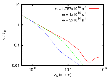
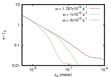
Figure 7: (Color online) Plot of the standard deviation $\sigma_{\perp}$ (left) and $\sigma_{\parallel}$ (right) for different distances of an atom placed at the distance $z_{\rm A}$ above a rough SiC surface with $\delta=5\,{\rm nm}$ and $a=200\,{\rm nm}$. The transition frequencies are chosen to be $\omega_{0}=1\cdot 10^{14}\,{\rm s}^{-1},1.787\cdot 10^{14}\,{\rm s}^{-1}$ and $3\cdot 10^{14}\,{\rm s}^{-1}$.

IV.4 LDOS fluctuations and $C_{0}$ correlation

Finally we want to explore the relation between the LDOS and the infinite range intensity correlation $C_{0}$ as studied for multiple scattering media Shapiro1999 . It was shown that this infinite range correlation equals the LDOS fluctuations VanTiggelen2006 . Since the decay rate is proportional to the LDOS, one could expect by analogy that above a rough surface the $C_{0}$ correlation equals the decay rate fluctuations or more precisely $C_{0}=\sigma^{2}/\langle\Gamma\rangle^{2}$. To prove this, we follow the reasoning of Ref. CazeEtAl2010 adapted to our problem. First we assume for simplicity that we have a non-absorbing half-space with a rough surface. Then the radiated power of a dipole in vacuum $P_{0}$ and of a dipole above the rough surface $P$ can be related to the decay rate of an atom in vacuum $\Gamma_{0}$ and the decay rate of an atom above a rough surface $\Gamma$ by the simple relation NovotnyHecht2006

$$\frac{P}{P_{0}}=\frac{\Gamma}{\Gamma_{0}}.$$ (27)

Since the decay rate is proportional to the LDOS $\rho$ at the position of the atom we also have $P/P_{0}=\rho/\rho_{0}$.

Now, we define the speckle correlation function $C(\mathbf{x,x^{\prime}})$ for the lateral correlations with respect to $\mathbf{x}$ and $\mathbf{x}^{\prime}$ above the surface as

$$C(\mathbf{x,x^{\prime}})=\frac{\langle I(\mathbf{x})I(\mathbf{x}^{\prime})\rangle}{\langle I(\mathbf{x})\rangle\langle I(\mathbf{x}^{\prime})\rangle}-1$$ (28)

where $I(\mathbf{x})$ is the radiated power of the dipole at the position $\mathbf{x}$ such that the integral over a plane parallel to the mean surface at $z=0$ (but for $z>z_{\rm A}$ and $z>\lambda_{0}$ so that evanescent waves are not included)

$$\lim_{r_{0}\rightarrow\infty}\frac{1}{A}\int_{A}{\rm d}^{2}x\,I(\mathbf{x})=P\cdot R$$ (29)

gives the total radiated power into the halfspace for $z>z_{\rm A}$. Here, we have introduced the circular area $A=\pi r_{0}^{2}$. The factor $R$ takes into account that only a part of the total power $P$ is radiated into the halfspace for $z>z_{\rm A}$, whereas another part $P\cdot T$ is radiated into the halfspace $z<0$ such that the total power is the sum of both contributions, i.e., $T+R=1$.

With the relation $P/P_{0}=\rho/\rho_{0}$ and the definition of $I(\mathbf{x})$ and $C(\mathbf{x,x^{\prime}})$ we have

$$\begin{split}\biggl{\langle}\frac{\rho^{2}}{\rho_{0}^{2}}\biggr{\rangle}&=\lim_{r_{0}\rightarrow\infty}\frac{1}{A^{2}}\frac{1}{R^{2}}\frac{1}{P_{0}^{2}}\int_{A}{\rm d}^{2}x\int_{A}{\rm d}^{2}x^{\prime}\,\langle I(\mathbf{x})I(\mathbf{x}^{\prime})\rangle\\ &=\lim_{r_{0}\rightarrow\infty}\frac{1}{A^{2}}\frac{1}{R^{2}}\frac{1}{P_{0}^{2}}\int_{A}{\rm d}^{2}x\int_{A}{\rm d}^{2}x^{\prime}\,\langle I(\mathbf{x})\rangle\langle I(\mathbf{x}^{\prime})\rangle\bigl{[}C(\mathbf{x,x^{\prime}})+1\bigr{]}.\end{split}$$ (30)

Since after averaging we retrieve the translational invariance parallel to the plane with $z=0$ and isotropy, we have $\langle I(\mathbf{x})\rangle=P\cdot R=P_{0}\cdot R\rho/\rho_{0}$. Inserting this relation into (30) it follows that

$$\begin{split}\langle\rho^{2}\rangle&=\langle\rho\rangle^{2}\lim_{r_{0}\rightarrow\infty}\frac{1}{A^{2}}\int_{A}{\rm d}^{2}x\int_{A}{\rm d}^{2}x^{\prime}\,\bigl{[}1+C(|\mathbf{x-x^{\prime}}|)\bigr{]}\\ &=\langle\rho\rangle^{2}\biggl{[}1+\lim_{r_{0}\rightarrow\infty}\frac{2\pi}{A}\int_{0}^{\infty}{\rm d}r\,rC(r)\biggr{]}.\end{split}$$ (31)

In fact, the integral over $C(r)$ gives nonzero contributions only for $C(r)={\rm const}\equiv C_{0}$, when assuming that for intensity correlations the relation $C(0)\geq C(r)$ for $r>0$ is valid. Therefore the integral in Eq. (31) reduces to $C_{0}$, i.e., the constant component of $C(r)$ which is the searched for infinite range $C_{0}$ correlation. Hence, we find

$$C_{0}=\frac{\langle\rho^{2}\rangle-\langle\rho\rangle^{2}}{\langle\rho\rangle^{2}}=\frac{\langle\Gamma^{2}\rangle-\langle\Gamma\rangle^{2}}{\langle\Gamma\rangle^{2}},$$ (32)

which proves our statement that the $C_{0}$ correlation equals the decay rate fluctuations or $C_{0}=\sigma^{2}/\langle\Gamma\rangle^{2}$.

Finally, using the perturbation expansion for the decay rate, we get for the $C_{0}$ correlations above a rough surface

$$C_{0}=\frac{\sigma^{2}}{\langle\Gamma\rangle^{2}}\approx\frac{\langle\Gamma^{(1)}\Gamma^{(1)}\rangle}{\bigl{(}\Gamma^{(0)}+\langle\Gamma^{(2)}\rangle\bigr{)}^{2}}=\frac{\langle\Gamma^{(1)}\Gamma^{(1)}\rangle}{{\Gamma^{(0)}}^{2}}\frac{1}{\biggl{(}1+\frac{\langle\Gamma^{(2)}\rangle}{\Gamma^{(0)}}\biggr{)}^{2}}\approx\frac{\langle\Gamma^{(1)}\Gamma^{(1)}\rangle}{{\Gamma^{(0)}}^{2}}.$$ (33)

Hence, the square of the normalized standard deviation $\sigma/\Gamma^{(0)}$ gives the infinite range $C_{0}$ correlation showing its sensitivity to the local environment which enters through its dependence on $z_{\rm A}$. In the quasi-static regime, we can now use the above derived result in Eq. (26) so that for $z_{\rm A}\ll a$ we find $C_{0}\approx 9\delta^{2}/z^{2}_{\rm A}$. We note that this result is very similar to the result found by Shapiro Shapiro1999 for random media, where $C_{0}=\pi/(kl)$ with the wave number $k$ and the mean free path of radiation inside the random medium $l$. In our case, $\delta^{2}/z_{\rm A}^{2}$ corresponds to the scattering strength $1/(kl)$.

V Conclusion

We have studied the impact of surface roughness on the decay rate or inverse lifetime of a molecule or atom above a rough surface. For pedagogical reasons we have only considered SiC as the bulk material, but the conclusions can be easily transfered to other dielectric materials supporting surface modes as for example silica. Our results show that the decay rate might be reduced by $15\%$ due to the surface roughness for very shallow roughnesses with an rms of $\delta=5\,{\rm nm}$ and a correlation length of $a=200\,{\rm nm}$. This reduction is due to the surface induced scattering of surface modes which prevails for intermediate distances. On the other hand, for very small distances $z_{\rm A}\ll a$ the rouhgness correction to the decay rate $\Gamma^{(0)}$ is due to the local electrostatic interaction of the atom or molecule with the surface and is given by the simple expression $6\delta^{2}/z_{\rm A}^{2}\Gamma^{(0)}$.

In addition, we have studied the variance and the lateral correlation of decay rates above the rough surface. We find that the lateral correlation length is approximately given by the distance $z_{\rm A}$ itself in the nonretarded regime for distances larger than $a$. For distances smaller than $a$ the lateral correlation function resembles the surface roughness correlation function allowing for a direct measurement of the surface roughness properties by measuring decay rate or lifetime correlations. The variance itself is a special case of the lateral correlation function and we have pointed out that it equals the $C_{0}$ correlation as for random media. We have shown that it can also be approximated by a simple result $\sigma^{2}=9\delta^{2}/z_{\rm A}^{2}$ in the quasistatic regime for $z_{\rm A}\ll a$ emphasizing that the infinite range $C_{0}$ correlation highly depends on the local environment of the atom, i.e., on the distance $z_{\rm A}$.

Appendix A Green’s function for a flat surface

The Green’s function with observation point and source point above the flat surface, i.e., for $0<z\leq z^{\prime}$ can be stated as Sipe1987 ; HenkelSandoghdar1998

$$\begin{split}\mathds{G}^{(0)}(\mathbf{r,r^{\prime}};\omega)&=\int\!\!\!\frac{{\rm d}^{2}\kappa}{(2\pi)^{2}}\frac{{\rm i}{\rm e}^{{\rm i}\boldsymbol{\kappa\cdot(\mathbf{x-x^{\prime}})}}}{2\gamma_{\rm r}}\biggl{[}\mathds{1}_{--}{\rm e}^{{\rm i}\gamma_{\rm r}(z^{\prime}-z)}+\mathds{R}_{+-}{\rm e}^{{\rm i}\gamma_{\rm r}(z^{\prime}+z)}\biggr{]}\\ &\quad-\frac{1}{3k_{0}^{2}}\delta(z-z^{\prime})\delta(\mathbf{x-x^{\prime}})\mathbf{e}_{z}\otimes\mathbf{e}_{z}\end{split}$$ (34)

where $\mathbf{e}_{z}$ is the unit vector in z-direction and $\otimes$ symbolizes the dyadic product. The tensors $\mathds{1}$ and $\mathds{R}$ are defined as

$$\mathds{1}_{--} =\sum_{j=\{{\rm s},{\rm p}\}}\hat{\mathbf{a}}_{j}^{-}(\boldsymbol{\kappa})\otimes\hat{\mathbf{a}}_{j}^{-}(\boldsymbol{\kappa})$$ (35)

$$\mathds{R}_{+-} =\sum_{j=\{{\rm s},{\rm p}\}}r_{j}\hat{\mathbf{a}}_{j}^{+}(\boldsymbol{\kappa})\otimes\hat{\mathbf{a}}_{j}^{-}(\boldsymbol{\kappa})$$ (36)

where

$$\hat{\mathbf{a}}_{\rm s}^{-}(\boldsymbol{\kappa}) =\hat{\mathbf{a}}_{\rm s}^{+}(\boldsymbol{\kappa})=\frac{1}{\kappa}(-k_{y},k_{x},0)^{\rm t},$$ (37)

$$\hat{\mathbf{a}}_{\rm p}^{-}(\boldsymbol{\kappa}) =-\frac{1}{\kappa k_{0}}(k_{x}\gamma_{\rm r},k_{y}\gamma_{\rm r},\kappa^{2})^{\rm t},$$ (38)

$$\hat{\mathbf{a}}_{\rm p}^{+}(\boldsymbol{\kappa}) =\frac{1}{\kappa k_{0}}(k_{x}\gamma_{\rm r},k_{y}\gamma_{\rm r},-\kappa^{2})^{\rm t}$$ (39)

are the polarization vectors for s- and p-polarization. Note that these vectors are always orthogonal, but only normalized for propagating modes with $\kappa<k_{0}$. The reflection coefficients $r_{\rm s}$ and $r_{\rm p}$ are the usual Fresnel coefficients

$$r_{\rm s}=\frac{\gamma_{\rm r}-\gamma_{\rm t}}{\gamma_{\rm r}+\gamma_{\rm t}}\quad\text{and}\quad r_{\rm p}=\frac{\gamma_{\rm r}\epsilon-\gamma_{\rm t}}{\gamma_{\rm r}\epsilon+\gamma_{\rm t}}.$$ (40)

Appendix B First-order Green’s function

The correction to the Green’s function we find from first-order perturbation theory is Greffet1988

$$\mathds{G}^{(1)}(\mathbf{r,r^{\prime}};\omega)=-\int\!\!\!\frac{{\rm d}^{2}\kappa}{(2\pi)^{2}}\int\!\!\!\frac{{\rm d}^{2}\kappa^{\prime}}{(2\pi)^{2}}\frac{k_{0}^{2}(\epsilon-1)}{4\gamma_{\rm r}\gamma_{\rm r}^{\prime}}{\rm e}^{{\rm i}(\boldsymbol{\kappa}\cdot\mathbf{x}+\gamma_{\rm r}z)}\tilde{S}^{(1)}(\boldsymbol{\kappa}^{\prime}-\boldsymbol{\kappa}){\rm e}^{{\rm i}(\boldsymbol{\kappa}^{\prime}\cdot\mathbf{x}^{\prime}+\gamma_{\rm r}^{\prime}z^{\prime})}\mathds{X}_{+-}(\boldsymbol{\kappa},\boldsymbol{\kappa}^{\prime})$$ (41)

with

$$\tilde{S}^{(1)}(\boldsymbol{\kappa}^{\prime}-\boldsymbol{\kappa})=\int\!\!{\rm d}^{2}x\,{\rm e}^{-i(\boldsymbol{\kappa}^{\prime}-\boldsymbol{\kappa})\cdot\mathbf{x}}S(\mathbf{x}).$$ (42)

and

$$\mathds{X}_{+-}(\boldsymbol{\kappa},\boldsymbol{\kappa}^{\prime})=\sum_{i,j=\{{\rm s},{\rm p}\}}\hat{\mathbf{a}}^{+}_{i}(\boldsymbol{\kappa})\otimes\hat{\mathbf{a}}^{-}_{j}(\boldsymbol{\kappa}^{\prime})X_{ij}(\boldsymbol{\kappa},\boldsymbol{\kappa}^{\prime}).$$ (43)

The elements of the tensor $X_{ij}$ are given as

$$X_{{\rm s}{\rm s}} =t_{\rm s}t_{\rm s}^{\prime}\hat{\boldsymbol{\kappa}}\cdot\hat{\boldsymbol{\kappa}}^{\prime}$$ (44)

$$X_{{\rm s}{\rm p}} =-t_{\rm s}t_{\rm p}^{\prime}\frac{\gamma_{\rm t}^{\prime}}{\sqrt{\epsilon}k_{0}}\mathbf{e}_{z}\cdot\hat{\boldsymbol{\kappa}}\times\hat{\boldsymbol{\kappa}}^{\prime}$$ (45)

$$X_{{\rm p}{\rm s}} =-t_{\rm p}t_{\rm s}^{\prime}\frac{\gamma_{\rm t}}{\sqrt{\epsilon}k_{0}}\mathbf{e}_{z}\cdot\hat{\boldsymbol{\kappa}}\times\hat{\boldsymbol{\kappa}}^{\prime}$$ (46)

$$X_{{\rm p}{\rm p}} =+t_{\rm p}t_{\rm p}^{\prime}\frac{1}{\epsilon k_{0}^{2}}(\kappa\kappa^{\prime}\epsilon-\gamma_{\rm t}\gamma_{\rm t}^{\prime}\hat{\boldsymbol{\kappa}}\cdot\hat{\boldsymbol{\kappa}}^{\prime})$$ (47)

where $\hat{\boldsymbol{\kappa}}=\boldsymbol{\kappa}/\kappa$ and $t_{\rm s},t_{\rm p}$ are the usual amplitude transmission coefficients

$$t_{\rm s}=\frac{2\gamma_{\rm r}}{\gamma_{\rm r}+\gamma_{\rm t}}\qquad\text{and}\qquad t_{\rm p}=\frac{2\gamma_{\rm r}\sqrt{\epsilon}}{\gamma_{\rm r}\epsilon+\gamma_{\rm t}}.$$ (48)

Appendix C Correlation function

By inserting the Green’s function from Eq. (41) into Eq. (1) we find for the first-order correction to the decay rate the expression

$$\frac{\Gamma^{(1)}_{i}(\mathbf{r})}{\Gamma_{\infty}}=\frac{3\pi{\rm i}}{k_{0}}\int\!\!\frac{{\rm d}^{2}\kappa}{(2\pi)^{2}}\int\!\!\frac{{\rm d}^{2}\kappa^{\prime}}{(2\pi)^{2}}\bigl{[}\tilde{S}^{(1)}(\boldsymbol{\kappa}^{\prime}-\boldsymbol{\kappa})a_{i}(\boldsymbol{\kappa},\boldsymbol{\kappa}^{\prime};\mathbf{r})\\ -\tilde{S}^{(1)}(\boldsymbol{\kappa}-\boldsymbol{\kappa}^{\prime})a_{i}^{*}(\boldsymbol{\kappa},\boldsymbol{\kappa}^{\prime};\mathbf{r})\bigr{]}{\rm e}^{{\rm i}\mathbf{x}\cdot(\boldsymbol{\kappa}-\boldsymbol{\kappa}^{\prime})}$$ (49)

where

$$a_{i}(\boldsymbol{\kappa},\boldsymbol{\kappa}^{\prime};\mathbf{r})=\frac{k_{0}^{2}(\epsilon-1)}{4\gamma_{\rm r}\gamma_{\rm r}^{\prime}}{\rm e}^{{\rm i}z(\gamma_{\rm r}+\gamma_{\rm r}^{\prime})}\bigl{[}\mathbf{e}_{i}^{\rm t}\cdot\mathds{X}_{+-}\cdot\mathbf{e}_{i}\bigr{]}.$$ (50)

With this definition at hand it is an easy task to check that the correlation function is

$$\begin{split}\frac{\bigl{\langle}\Gamma^{(1)}_{i}(\mathbf{r})\Gamma^{(1)}_{j}(\mathbf{r}^{\prime})\bigr{\rangle}}{\Gamma_{\infty}^{2}}&=\frac{(3\pi)^{2}}{k_{0}^{2}}2{\rm Re}\int\!\!\frac{{\rm d}^{2}\kappa}{(2\pi)^{2}}\int\!\!\frac{{\rm d}^{2}\kappa^{\prime}}{(2\pi)^{2}}\delta^{2}g(|\boldsymbol{\kappa}-\boldsymbol{\kappa}^{\prime}|)a_{i}(\boldsymbol{\kappa},\boldsymbol{\kappa}^{\prime};\mathbf{r})\\ &\quad\times\int\!\!\frac{{\rm d}^{2}\kappa^{\prime\prime}}{(2\pi)^{2}}[a_{j}^{*}(\boldsymbol{\kappa}^{\prime\prime},\boldsymbol{\kappa}^{-};\mathbf{r}^{\prime})-a_{j}(\boldsymbol{\kappa}^{\prime\prime},\boldsymbol{\kappa}^{+};\mathbf{r}^{\prime})]{\rm e}^{{\rm i}(\mathbf{x}-\mathbf{x}^{\prime})\cdot(\boldsymbol{\kappa}-\boldsymbol{\kappa}^{\prime})}\end{split}$$ (51)

using the relations

$$\boldsymbol{\kappa}^{+}=\boldsymbol{\kappa}^{\prime\prime}+(\boldsymbol{\kappa}-\boldsymbol{\kappa}^{\prime}),$$ (52)

$$\boldsymbol{\kappa}^{-}=\boldsymbol{\kappa}^{\prime\prime}-(\boldsymbol{\kappa}-\boldsymbol{\kappa}^{\prime}).$$ (53)

By introducing the new variable $\boldsymbol{\xi}=\boldsymbol{\kappa}-\boldsymbol{\kappa}^{\prime}$ we can write the correlation function as

$$\frac{\bigl{\langle}\Gamma^{(1)}_{i}(\mathbf{r})\Gamma^{(1)}_{j}(\mathbf{r}^{\prime})\bigr{\rangle}}{\Gamma_{\infty}^{2}}=\frac{(3\pi)^{2}}{k_{0}^{2}}2{\rm Re}\int\!\!\frac{{\rm d}^{2}\xi}{(2\pi)^{2}}\delta^{2}g(|\boldsymbol{\xi}|)F_{j}(\boldsymbol{\xi};z^{\prime})G_{i}(\boldsymbol{\xi};z){\rm e}^{{\rm i}\boldsymbol{\xi}\cdot(\mathbf{x}-\mathbf{x}^{\prime})}$$ (54)

with

$$G_{i}(\boldsymbol{\xi};z)=\int\!\!\frac{{\rm d}^{2}\kappa}{(2\pi)^{2}}a_{i}(\boldsymbol{\kappa},\boldsymbol{\kappa}-\boldsymbol{\xi};z)$$ (55)

and

$$F_{j}(\boldsymbol{\xi};z^{\prime})=G_{j}^{*}(\boldsymbol{\xi};z^{\prime})-G_{j}(-\boldsymbol{\xi};z^{\prime}).$$ (56)

Appendix D Approximations for quasi-static limit

In the quasi-static limit ($\kappa\gg k_{0}$) the reflection coefficients can be approximated by

$$r_{\rm p}\approx\frac{\epsilon-1}{\epsilon+1}\quad\text{and}\quad r_{\rm s}\approx\frac{\epsilon-1}{4}\frac{k_{0}^{2}}{\kappa^{2}}.$$ (57)

By inserting these relations into Eqs. (55) we find the quasi-static approximations for the decay rates

$$\frac{\Gamma^{(0)}_{\parallel}}{\Gamma_{\infty}} \approx\frac{3}{16}\frac{1}{(k_{0}z)^{3}}{\rm Im}\biggl{(}\frac{\epsilon-1}{\epsilon+1}\biggr{)},$$ (58)

$$\frac{\Gamma^{(0)}_{\perp}}{\Gamma_{\infty}} \approx\frac{3}{8}\frac{1}{(k_{0}z)^{3}}{\rm Im}\biggl{(}\frac{\epsilon-1}{\epsilon+1}\biggr{)}.$$ (59)

In particular, $\Gamma_{\perp}^{(0)}=2\Gamma_{\parallel}^{(0)}$.

i) distance regime $z\ll a$

Now, we want to find similar simple approximate expressions for the correlation function in Eq. (54). To this end we consider first $\kappa\gg\xi$, which is fulfilled for $z\ll a$. For such wave vectors we can approximate Eq. (55) by

$$G_{\parallel}(\boldsymbol{\xi};z) \approx\int\!\!\frac{{\rm d}\kappa}{2\pi}\,\frac{k_{0}^{2}(\epsilon-1)}{8\gamma_{\rm r}^{2}}{\rm e}^{2{\rm i}\gamma_{\rm r}z}\biggl{(}t_{\rm s}^{2}-\frac{t_{\rm p}^{2}}{\epsilon k_{0}^{2}}\frac{\gamma_{\rm r}^{2}}{k_{0}^{2}}\bigl{[}\kappa^{2}(\epsilon+1)-k_{0}^{2}\epsilon\bigr{]}\biggr{)},$$ (60)

$$G_{\perp}(\boldsymbol{\xi};z) \approx\int\!\!\frac{{\rm d}\kappa}{2\pi}\,\frac{k_{0}^{2}(\epsilon-1)}{4\gamma_{\rm r}^{2}}{\rm e}^{2{\rm i}\gamma_{\rm r}z}\frac{t_{\rm p}^{2}}{\epsilon k_{0}^{2}}\frac{-\kappa^{2}}{k_{0}^{2}}\bigl{[}\kappa^{2}(\epsilon+1)-k_{0}^{2}\epsilon\bigr{]}.$$ (61)

Using the quasi-static approximation for the transmission coefficients

$$t_{\rm s}\approx 1\quad\text{and}\quad t_{\rm p}\approx\frac{2\sqrt{\epsilon}}{\epsilon+1}$$ (62)

allows for further simplification. We find

$$G_{\parallel}(\boldsymbol{\xi};z) \approx-\frac{3!}{4\pi}\frac{1}{(2z)^{4}}\frac{1}{k_{0}^{2}}\frac{\epsilon-1}{\epsilon+1},$$ (63)

$$G_{\perp}(\boldsymbol{\xi};z) \approx-\frac{3!}{2\pi}\frac{1}{(2z)^{4}}\frac{1}{k_{0}^{2}}\frac{\epsilon-1}{\epsilon+1}.$$ (64)

Inserting these approximations into Eq. (54) finally yields

$$\frac{\bigl{\langle}\Gamma^{(1)}_{\parallel}(\mathbf{r})\Gamma^{(1)}_{\parallel}(\mathbf{r}^{\prime})\bigr{\rangle}}{\Gamma_{\infty}^{2}} \approx\frac{81}{256}\frac{\delta^{2}}{k_{0}^{6}z^{4}{z^{\prime}}^{4}}\biggl{[}{\rm Im}\biggl{(}\frac{\epsilon-1}{\epsilon+1}\biggr{)}\biggr{]}^{2}W(|\mathbf{x-x^{\prime}}|),$$ (65)

$$\frac{\bigl{\langle}\Gamma^{(1)}_{\perp}(\mathbf{r})\Gamma^{(1)}_{\perp}(\mathbf{r}^{\prime})\bigr{\rangle}}{\Gamma_{\infty}^{2}} \approx\frac{81}{64}\frac{\delta^{2}}{k_{0}^{6}z^{4}{z^{\prime}}^{4}}\biggl{[}{\rm Im}\biggl{(}\frac{\epsilon-1}{\epsilon+1}\biggr{)}\biggr{]}^{2}W(|\mathbf{x-x^{\prime}}|).$$ (66)

As can be expected from $G_{\perp}=2G_{\parallel}$ we find

$$\frac{\bigl{\langle}\Gamma^{(1)}_{\perp}(\mathbf{r})\Gamma^{(1)}_{\perp}(\mathbf{r}^{\prime})\bigr{\rangle}}{\bigl{\langle}\Gamma^{(1)}_{\parallel}(\mathbf{r})\Gamma^{(1)}_{\parallel}(\mathbf{r}^{\prime})\bigr{\rangle}}=4.$$ (67)

ii) distance regime $z\gg a$

In this limit, we consider the case $\kappa\gg\xi$ yielding

$$G_{\perp} \approx\int\frac{{\rm d}^{2}\kappa}{(2\pi)^{2}}a_{z}(\boldsymbol{\kappa},-\boldsymbol{\xi}),$$ (68)

$$G_{\parallel} \approx\int\frac{{\rm d}^{2}\kappa}{(2\pi)^{2}}a_{x}(\boldsymbol{\kappa},-\boldsymbol{\xi}).$$ (69)

Together with the quasi-static approximation, i.e, $\xi\gg k_{0}$ and $\xi\gg k_{0}\epsilon$ we get

$$G_{\perp}\approx{\rm e}^{-\xi z}\xi\int\frac{{\rm d}\kappa}{2\pi}\kappa^{3}\frac{t_{\rm p}(\epsilon-1)}{k_{0}^{2}4{\rm i}\gamma_{\rm r}}{\rm e}^{{\rm i}\gamma_{\rm r}z}\frac{2\sqrt{\epsilon}}{\epsilon+1}\equiv f_{\perp}(z){\rm e}^{-\xi z}\xi$$ (71)

and

$$G_{\parallel}\approx{\rm e}^{-\xi z}\xi\cos^{2}(\theta)\frac{1}{2}\int\frac{{\rm d}\kappa}{2\pi}\kappa\frac{k_{0}^{2}(\epsilon-1)}{4{\rm i}\gamma_{\rm r}}{\rm e}^{{\rm i}\gamma_{\rm r}z}\biggl{[}\frac{\gamma_{\rm r}\gamma_{\rm t}t_{\rm p}}{k_{0}^{2}\epsilon}-\frac{r_{\rm s}}{k_{0}^{2}\sqrt{\epsilon}}\biggr{]}\equiv f_{\parallel}(z){\rm e}^{-\xi z}\xi\cos^{2}(\theta)$$ (72)

where we have introduced $\xi_{x}=\xi\cos{\theta}$ and $\xi_{y}=\xi\sin(\theta)$. Finally, when plugging these results into Eq. (51) we find GradshteynRyzhik2007

$$\frac{\bigl{\langle}\Gamma^{(1)}_{\perp}(\mathbf{x})\Gamma^{(1)}_{\perp}(\mathbf{x}^{\prime})\bigr{\rangle}}{\Gamma_{\infty}^{2}} \propto\frac{a^{2}\delta^{2}}{[z^{2}+|\mathbf{x}-\mathbf{x}^{\prime}|^{2}]^{2}}P_{3}\biggl{(}\frac{z}{\sqrt{z^{2}+(\mathbf{x}-\mathbf{x}^{\prime})^{2}}}\biggr{)},$$ (73)

$$\frac{\bigl{\langle}\Gamma^{(1)}_{\parallel}(\mathbf{x})\Gamma^{(1)}_{\parallel}(\mathbf{x}^{\prime})\bigr{\rangle}}{\Gamma_{\infty}^{2}} \propto\frac{\delta^{2}a^{2}}{z^{4}}\biggl{[}\,\tensor{[}_{2}]{F}{{}_{1}}\biggl{(}2,\frac{5}{2};3;-\frac{|\mathbf{x}-\mathbf{x}^{\prime}|^{2}}{z^{2}}\biggr{)}$$

$$\qquad-\frac{20}{3}\,\frac{|\mathbf{x}-\mathbf{x}^{\prime}|^{2}}{z^{2}}\tensor{[}_{2}]{F}{{}_{1}}\biggl{(}3,\frac{7}{2};3;-\frac{|\mathbf{x}-\mathbf{x}^{\prime}|^{2}}{z^{2}}\biggr{)}\biggr{]}$$ (74)

where $P_{3}$ is the Legendre polynomial of third power and $\tensor{[}_{2}]{F}{{}_{1}}$ is the hypergeometric function.

References

- (1) E. M. Purcell, Phys. Rev. 69, 681 (1946).
- (2) K. H. Drexhage, H. Kuhn, and F. P. Schäfer, Ber. Bunsenges. phys. Chem. 72, 1179 (1968).
- (3) G. W. Ford and W. H. Weber, Phys. Rep. 113, 195 (1984).
- (4) W. L. Barnes, J. Mod. Opt. 45, 661 (1998).
- (5) B. Shapiro, Phys. Rev. Lett. 57, 2168 (1986).
- (6) B. Shapiro, Phys. Rev. Lett. 83, 4733 (1999).
- (7) B. A. van Tiggelen and S. E. Skipetrov, Phys. Rev E 73, 045601(R) (2006).
- (8) A. Cazé, R. Pierrat, and R. Carminati, Phys. Rev. A 82, 043823 (2010).
- (9) L.S. Froufe-Pérez, R. Carminati, and J. J. Sáenz, Phys. Rev. A 76, 013835 (2007).
- (10) P. V. Ruijgrok, R. Wüest, A. A. Rebane, A. Renn, and V. Sandoghdar, Opt. Exp. 18, 6360 (2010).
- (11) M. D. Birowosuto, S. E. Skipetrov, W. L. Vos, and A. P. Mosk, Phys. Rev. Lett. 105, 013904 (2010).
- (12) R. Sapienza, P. Bondareff, R. Pierrat, B. Habert, R. Carminati, and N. F. van Hulst, Phys. Rev. Lett. 106, 163902 (2011).
- (13) V. Krachmalnicoff, E. Castanié, Y. De Wilde, and R. Carminati, Phys. Rev. Lett. 105, 183901 (2010).
- (14) J.-J. Greffet and R. Carminati, Ultramicroscopy 61, 43 (1995).
- (15) A. Apostol and A. Dogariu, Phys. Rev. Lett. 91, 093901 (2003).
- (16) A. Apostol and A. Dogariu, Phys. Rev. E 67, 055601(R) (2003).
- (17) R. Carminati, Phys. Rev. A 81, 053804 (2010).
- (18) K. Arya, R. Zeyher and A. A. Maradudin, Sol. State Commun. 42, 461 (1981).
- (19) P. K. Aravind and H. Metiu, Chem. Phys. Lett. 74, 301 (1980).
- (20) J. Arias, P. K. Aravind, and H. Metiu, Chem. Phys. Lett. 85, 404 (1982).
- (21) Xiao-shen Li, D. L. Lin, and T. F. George, Phys. Rev. B 41, 8107 (1990).
- (22) J. E. Sipe, Surf. Sci. 84, 75 (1979).
- (23) B. N. J. Persson and N. D. Lang, Phys. Rev. B 26, 5409 (1982).
- (24) Ph. Avouris, D. Schmeisser, and J. E. Demuth, J. Chem. Phys. 79, 488 (1983).
- (25) F. Balzer, V. G. Bordo, and H.-G. Rubahn, Opt. Lett. 22, 1262 (1997).
- (26) C. F. Bohren, D. R. Huffman, Absorption and Scattering of Light by Small Particles, (John Wiley and sons, Inc., 1983).
- (27) J.-J. Greffet, Phys. Rev. B 37, 6436 (1988).
- (28) L. Novotny and B. Hecht, Principles of Nano-Optics, (Cambridge University Press,Cambridge,2006).
- (29) S.-A. Biehs and J.-J. Greffet, Phys. Rev. B 81, 245414 (2010).
- (30) J. A. DeSanto, Scalar wave theory, (Springer-Verlag, Heidelberg, 1992).
- (31) H. Raether Surface Plasmons on Smooth and Rough Surfaces and on Gratings, (Springer-Verlag, Heidelberg, 1988).
- (32) V. Emiliani, F. Intonti, M. Cazayous, D. S. Wiersma, M. Colocci, F. Aliev, and A. Lagendijk, Phys. Rev. Lett. 90, 250801 (2003).
- (33) J. Laverdant, S. Buil, B. Bérini, and X. Quélin, Phys. Rev. B 77, 165406 (2008).
- (34) R. Carminati, Phys. Rev. A 81, 053804 (2010).
- (35) S. I. Bozhevolnyi, B. Vohnsen, I. I. Smolyaninov, and A. V. Zayats, Opt. Commun. 117 (1995).
- (36) S. I. Bozhevolnyi, A. V. Zayats, and B. Vohnsen, Optics at the Nanometer Scale, (Kluwer, Dordrecht, 1996).
- (37) S. I. Bozhevolnyi and V. Coello, Phys. Rev. B 64, 115414 (2001).
- (38) S. Buil, J. Aubineau, J. Laverdant, and X. Quélin, J. Appl. Phys. 100, 063530 (2006).
- (39) J. A. Sánchez-Gil, J. V. Garciá-Ramos, and E. R. Méndez, Phys. Rev. B 62, 10515 (2000).
- (40) J. A. Sánchez-Gil, J. V. Garciá-Ramos, and E. R. Méndez, Opt. Lett. 26, 1286 (2001).
- (41) J. E. Sipe, J. Opt. Soc. Am. B 4, 481 (1987).
- (42) I. S. Gradshteyn and I. M. Ryzhik, Table of Integrals, Series and Products, (Academic Press, San Diego, 2007).
- (43) C. Henkel and V. Sandoghdar, Opt. Commun. 158, 250 (1998).