Performance Analysis of Sequential Method for Handover in Cognitive Radio Networks

Abstract

Powerful spectrum handover schemes enable cognitive radios (CRs) to use transmission opportunities in primary users’ channels appropriately. In this paper, we consider the cognitive access of primary channels by a secondary user (SU). We evaluate the average detection time and the maximum achievable average throughput of the SU when the sequential method for hand-over (SMHO) is used. We assume that a prior knowledge of the primary users’ presence and absence probabilities are available. In order to investigate the maximum achievable throughput of the SU, we end into an optimization problem, in which the optimum value of sensing time must be selected. In our optimization problem, we take into account the spectrum hand over due to false detection of the primary user. We also propose a weighted based hand-over (WBHO) scheme in which the impacts of channels conditions and primary users’ presence probability are considered. This spectrum handover scheme provides higher average throughput for the SU compared to the SMHO method. The tradeoff between the maximum achievable throughput and consumed energy is discussed, and finally an energy efficient optimization formulation for finding a proper sensing time is provided.

I Introduction

Emerging new wireless applications and ever-growing need to have a higher data rate have increased the demand for accessing to the spectrum in the past ten years, incredibly. Though the available spectrum resources seem not to meet the ever-growing demand, many investigations reveal that the spectrum is inefficiently used [1]. Cognitive radio (CR) concept has been introduced to improve spectrum efficiency by allowing the low-priority secondary users (SUs) to opportunistically exploit the unused licensed spectrum of the high-priority primary users (PUs) [1], [2]. To this end, first the spectrum holes must be found through appropriate and reliable spectrum sensing techniques. However, there are two challenges associated with spectrum sensing: (1) Limited Observations, and, (2) Time Variation. Since the numbers of samples used for sensing are limited, the idle spectrum cannot be detected perfectly. Moreover, due to stochastic nature of PUs activities, accessibility of the SUs to the spectrum is time variant. However, the SU enforce to stop its transmission and vacate the occupied channel when the PU has data to transmit on this channel. Within the transmission period of a secondary connection, it is likely to have multiple spectrum handoffs due to interruptions from the PUs. In order to provide reliable transmission for the SUs and guarantee some level of quality of service (QoS), a set of procedures called spectrum handover (HO) is initiated to help the SU to find a new transmission opportunity and resume its unfinished transmission [1], [3].

Generally, there exists more than one channel to be sensed by a CR. To deal with this fact, sensing schemes are commonly divided into two categories, i.e., wideband sensing and narrowband sensing. Sensing is wideband when multiple channels are sensed simultaneously. These multiple sensed channels can cover either the whole or a portion of the primary channels [4]. On the other hand, when only one channel is sensed at a time, the sensing process is narrowband. Ease of implementation, lower power consumption, and less computational complexity leads to great interest in narrowband sensing. When the narrowband sensing is used, the channels have to be sensed in a proper order called sensing sequence. Incorporating powerful spectrum sensing schemes enable SUs to transmit and/or receive data while no channels are dedicated to them. Average throughput of the SU, average sensing time, and consumed energy are some common metrics considered in designing appropriate sensing schemes.

Throughput maximization of the SUs has been widely investigated in the literature. Specifically, in [5] and [6] a set of procedures is proposed to determine the optimal set of candidate channels, and maximizing the spectrum accessibility through the optimal number of candidate channels is investigated. Minimizing the overall system time of a SU through load balancing in probability-based and sensing-based spectrum decision schemes is investigated in [7]. The joint design of sensing-channel selection and power control scheme is investigated in [8]. Assuming a perfect sensing scheme and static wireless channels, this joint optimization is formulated, and suboptimal algorithms with tolerable computational complexity are developed to approximately solve the derived optimization problem. The same problem is formulated in [9] considering the impact of time-varying fading channels as well as the sensing errors. The author derives a closed-form relation under the constraint of average available power and the level of collision with the PUs and develops a stochastic optimization approach. Throughput maximization through optimizing spectrum sensing time has gained a lot of interest. Spectrum sensing time is one of the most effective factors which must be determined carefully to obtain a powerful sensing scheme. In [10], [11], [12], and [13] the impact of spectrum sensing time on the overall throughput of the SUs is investigated. It is shown in [11] that as the sensing time increases, the sensing accuracy increases as well, but the throughput decreases; thus there is an interesting tradeoff. In [11], while the spectrum HOs effect has not been taken into account, the optimum value of the sensing time has been found numerically. When a PU arrives, the SU must leave the spectrum and continues its transmission on a free spectrum after possibly some HOs. Clearly, multiple spectrum HOs will increase the overall sensing time [12]. In [13] it is assumed that the licensed spectrums are numbered sequentially, and the SU starts to sense the spectrums from top of a list. In the case of occupation, the SU senses the next one, and this process is continued until an idle spectrum is found. Then, in [13], an optimization problem is formulated in order to minimize the average sensing time. Although the false detection and spectrum handover effects on sensing time have been investigated in [13], but the negative effect of the handover (equivalently the effect of multiple sensing time) on the SU throughput has not taken into account.

In this paper, we consider the energy detection (ED) method as PU detection scheme and try to set appropriate values for the ED’s parameters, i.e., sensing time $\tau$ and decision threshold $\lambda$. The same problem is formulated in [11] without considering the impact of HO on the derived average throughput. In fact, [11] assumes that the SU senses the one spectrum in each time-slot and transmits on it if it is sensed free. As mentioned before, there exist a trade-off on selecting a value for the sensing time, and thus an optimization problem can be formulated in order to choose an appropriate value for sensing time. It is shown in [11] that the two dimensional optimization problem (with respect to $\tau$ and $\lambda$) can be simplified to a one-dimensional with respect to $\tau$. However, in contrast to [11], as we are considering the spectrum mobility effect on the overall sensing time, we show that our problem cannot convert to a one-dimensional one. In this paper, we consider the sequential method for handover (SMHO) first introduced in [13]. We evaluate the average sensing time, the average number of required handover for a given maximum false alarm probability, and the average throughput of a SU temporarily used the spectrum allocated to $N_{p}$ primary users. We formulate an optimization problem in which the optimal sensing time for maximizing the SU throughput is obtained. Different from [11], we show that our problem cannot convert to a one-dimensional optimization problem. Then, we propose a weighted based scheme for handover (WBHO) as a trade-off between the complexity of finding an optimal handover sequence and the maximum achievable throughput of the SU. In the WBHO scheme considered, a weight is assigned to each primary channel based on the channel conditions and the PUs entrance probability in the next slots. Then, the algorithm decreasingly sorts these channels based on their weights. The WBHO scheme provides a higher average throughput and lower consumed energy to find a transmission opportunity compared to the SMHO.

The rest of this paper is organized as follows. Section II describes the system model. Problem formulation and performance analysis of the SMHO scheme are provided in Section III. In Section IV, channel imperfections such as fading is considered, and we develop a new weighted based handover framework. Numerical results are presented in Section V, and finally the paper concludes in Section VI.

II System Model

We consider one secondary user and $N_{p}$ primary users, and in each time-slot the SU user transmits on at most one of $N_{p}$ existing bands by using opportunistic methods. We assume the SU always has packets to transmit, and therefore it will start transmission when an opportunity is found. A thoroughly synchronous system is assumed in this paper in which the SU is synchronous in time-slots with the PUs. When a PU has no data for transmission it does not use it s time-slots, thus provides a transmission opportunity for the SU. But if the PU has data for transmission, it starts transmitting at the beginning of the next time-slot. In order to find the transmission opportunities appropriately and protecting the PUs from harmful interference, the sensing process must be performed at the beginning of each time-slot. We assume that the SU is equipped with a simple transceiver, so they are able to sense only one channel per time-slot. We also assume that there is a fixed time $\tau_{ho}$ for the SU detector to change its channel and switch to a new one independent of the channel frequency in which it switches. We assume that the different PUs activities are independent. The state of channel $i$ that used by $i$-th PU at time-slot t is denoted by $s_{i}(t)$:

$${s_{i}}\left(t\right)=\left\{{\begin{array}[]{*{20}{c}}{0{\rm{~{}}}:{\rm{~{}~{}if~{}channel~{}i~{}is~{}occupied\hfill}}}{}\\ {1{\rm{~{}}}:{\rm{~{}~{}if~{}channel~{}i~{}is~{}idle\hfill}}}{}\\ \end{array}}\right.$$ (1)

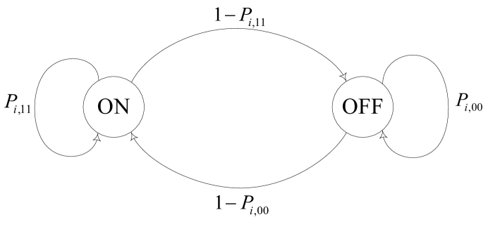
Figure 1: Graphical representation of ON-OFF primary user traffic model

The two state Markov model called ON-OFF traffic model, as shown in Fig. 1, can be used to model the correlation of a channel states [14], where ON and OFF states in Fig. 1 represent the presence and the absence of the $i$-th PU, i.e., $s_{i}=1$ and $s_{i}=0$, respectively. $P_{i,00}$ and $P_{i,11}$ are the probabilities that the channel state transits from idle (in the current slot) to idle (in the next slot) and from busy to busy, respectively. The transition probabilities of the PUs in the ON-OFF model can be determined according to traffic statistics from the long-term observation. Note that for $i$-th PU, the steady state idle probability of the channel $i$ can be calculated as:

$$\Pr\left\{{{s_{i}}\left(t\right)=0}\right\}={P_{i,0}}=\frac{{1-{P_{i,00}}}}{{2-{P_{i,00}}-{P_{i,11}}}}$$ (2)

Spectrum sensing can be formulated as a binary hypothesis testing problem [11],

$$\left\{{\begin{array}[]{*{20}{c}}{{\mathcal{H}_{0}~{}:~{}y(n)=z(n)}{\rm{~{}:~{}~{}channel~{}is~{}idle\hfill}}}\\ {{\mathcal{H}_{1}~{}:~{}y(n)=u(n)+z(n)}{\rm{~{}:~{}~{}channel~{}is~{}occupied\hfill}}}\\ \end{array}}\right.$$ (3)

where the noise $z(n)$ is zero mean complex-valued, independent and identically distributed (i.i.d) Gaussian sequence, $u(n)$ is the PUs signal and independent of $z(n)$, and $y(n)$ is the $n$-th sample of the received signal. Generally, there are various PU detection schemes such as match filtering, cyclostationary feature detection, waveform-based sensing, and energy detection (ED) [15],

among which the ED is the most prevalent because of its low complexity and ease of implementation. Further, it does not require any information about the PUs signal attributes [16]. By defining $X$ as a decision metric for the ED, we have,

$${X}=\sum\limits_{n=1}^{N}{{{\left|{y\left(n\right)}\right|}^{2}}}$$ (4)

where $X$ is the received energy in the detector. $N$ represents the number of samples that is equal to $N=\tau{f_{s}}$, where $\tau$ and $f_{s}$ are the sensing time and the sampling frequency, respectively. Finally, the decision criteria is defined as,

$$\left\{{\begin{array}[]{*{20}{c}}{X<\lambda{\rm{}}\equiv{\mathcal{H}_{0}\hfill}}\\ {X\geq\lambda{\rm{}}\equiv{\mathcal{H}_{1}\hfill}}\\ \end{array}}\right.$$ (5)

Let $\sigma_{u}^{2}$ denote the received energy of the PU signal, and $\sigma_{z}^{2}$ represent the noise variance, then the received signal to noise ratio due to the PU is computed as $\gamma=\frac{{\sigma_{u}^{2}}}{{\sigma_{z}^{2}}}$. Assume that $\lambda$ is the threshold of the ED decision rule, and $\overline{P_{d}}$ is the minimum allowable probability of detection. If the number of received signal’s samples is large enough, the statistical distribution of $X$ can be approximated by a Gaussian distribution, and then the detection and false alarm probabilities can be computed using the following formulas [11]:

$${P_{d}}=Q\left[{\left({\frac{\lambda}{{\sigma_{u}^{2}}}-1-\gamma}\right)\sqrt{\frac{{\tau{f_{s}}}}{{1+2\gamma}}}}\right]$$ (6)

$${P_{fa}}=Q\left[{\left({\frac{\lambda}{{\sigma_{u}^{2}}}-1}\right)\sqrt{\tau{f_{s}}}}\right],$$ (7)

where $P_{d}$ and $P_{fa}$ are the detection and false alarm probabilities, respectively. For ${P_{d}}=\overline{{P_{d}}}$, which $\overline{{P_{d}}}$ is a fixed amount, we obtain:

$$\lambda=\left({{Q^{-1}}\left({\overline{{P_{d}}}}\right)\sqrt{\frac{{1+2\gamma}}{{\tau{f_{s}}}}}+1+\gamma}\right)\sigma_{u}^{2}$$ (8)

Suppose that $\beta={Q^{-1}}\left({\overline{{P_{d}}}}\right)\sqrt{1+2\gamma}$, (8) is simplified to:

$${P_{fa}}=Q\left[{\beta+\gamma\sqrt{\tau{f_{s}}}}\right]$$ (9)

For the SU, each slot contains two phases: 1) sensing phase, and 2) transmission phase. The sensing phase contains several mini-slots of duration $\tau$ (sensing time of each channel). Sensing is carried out by the SU in mini-slots, and once the transmission opportunity is found, the transmission phase will be started. This kind of access, i.e., listen-before-talk (LBT) is a common method in many wireless communication systems; see e.g. the quiet period in IEEE 802.22 standard [17]. The sensing procedure is performed in an order based on the predefined sensing sequence. Given the primary-free probabilities, i.e., ${P_{0,j}}{\rm{~{}}},{\rm{~{}}}1\leq j\leq{N_{p}}$, in this paper we aim to formulate the performance of the SU for two kinds of the sensing sequence and find the optimal setting values for the ED

III Performance Analysis

In this section, we first consider the SMHO scheme and derive its performance, and then the WBHO scheme is addressed. As mentioned above, in the SMHO scheme, the SU arranges the frequency channels by their numbers. If HO is required, the SU must sense the spectrum from the top of the list and if it is sensed free, the SU begins to transmit on it. In other case, the SU senses the next spectrum, and this scenario continues until an idle spectrum is found.

First we compute the average number of HOs, denoted by $\overline{g}_{SMHO}$, to find an idle spectrum. The SU transmits on the $k$-th channel with the following probability,

$$\begin{array}[]{c}{q_{k}}=\Pr\left\{{{\rm{ED~{}says~{}}}1|{\mathcal{H}_{0}}}\right\}{P_{k,0}}+\Pr\left\{{{\rm{ED~{}says~{}}}1|{\mathcal{H}_{1}}}\right\}{P_{k,1}}\\ ={P_{fa}}{P_{k,0}}+{P_{d}}{P_{k,1}},\\ \end{array}$$ (10)

where ${P_{k,0}}$ and ${P_{k,1}}$ are the absence and presence probability of the $k$-th PU, respectively.

Lemma 1: The average number of HOs is equal to

$${\overline{g}_{SMHO}}={q_{1}}{\left(1-q_{2}\right)}+2{q_{1}}{q_{2}}{\left(1-q_{3}\right)}+\cdots+\left(\alpha-1\right)\left(1-q_{\alpha}\right)\prod\limits_{j=1}^{\alpha-1}{q_{j}}+\alpha\prod\limits_{j=1}^{\alpha}{{q_{j}}}$$ (11)

where $\alpha$ is the maximum number of allowable HOs.

Proof: According to the SMHO, if the SU transmits on the $i$-th spectrum, $\left(i-1\right)$ times hand over will be necessary. The probability of $\left(i-1\right)$ consecutive channel are sensed busy, and the $i$-th channel is sensed free is equal to $\left(1-q_{i}\right)\prod\limits_{k=1}^{i-1}{{q_{k}}}$. In addition, there are two constraints on the maximum number of HOs, the first one is due to the number of channels (or equivalently the number of PUs), where the number of sensed channels cannot exceed the number of the PUs, and the second is due to the time-slot period, where the sum of the elapsed times for both sensing and HO procedures can not exceed the time-slot duration. So, we have,

$$\alpha=\min\left({\left\lfloor{\frac{{T-\tau}}{{\tau+{\tau_{ho}}}}}\right\rfloor,{N_{P}}-1}\right){\rm{}}$$ (12)

where $\tau_{ho}$ is defined above and $T$ is the duration of each time-slot. Thus, the average number of HOs can be determined by (11).

Then, we can easily conclude the following lemma.

Lemma 2: The average time of spectrum sensing can be calculated as, $E\left\{{\rm{sensing~{}time}}\right\}=\tau+{\overline{g}_{SMHO}}\left({\tau+{\tau_{ho}}}\right)$.

In the following Lemma, the average achievable throughput has been given.

Lemma 3: Considering the maximum allowable number of HOs equal to $\alpha$, the average achievable normalized throughput can be calculated as,

$$R=\sum\limits_{m=0}^{\alpha}{\underbrace{\left({{C_{1}}{P_{m+1,1}}\left({1-{P_{d}}}\right)+{C_{0}}{P_{m+1,0}}\left({1-{P_{fa}}}\right)}\right)}_{T1}\underbrace{{q_{0}}{q_{1}}\cdots{q_{m}}\left({1-\frac{{\tau+m\left({\tau+{\tau_{ho}}}\right)}}{T}}\right)}_{T2}}$$ (13)

where ${q_{0}}\buildrel\Delta\over{=}1$, ${C_{0}}={\log_{2}}\left({1+{\gamma_{s}}}\right)$ and ${C_{1}}={\log_{2}}\left({1+\frac{{{P_{s}}}}{{{N_{0}}+{P_{p}}}}}\right)={\log_{2}}\left({1+\frac{{{\gamma_{s}}}}{{1+{\gamma_{p}}}}}\right)$ are the SU’s capacity under the hypothesis $\mathcal{H}_{0}$ and $\mathcal{H}_{1}$, respectively. ${\gamma_{s}}$ and ${\gamma_{p}}$ are the received SNRs due to the secondary and primary user s signals at the SU receiver, respectively, and $P_{k,0}$ is defined in (2).

Proof: The proof is given in appendix A.

The optimum throughput can be obtained by solving the following optimization problem $P1$:

$$\begin{array}[]{l}P1:{\rm{~{}~{}}}\mathop{\max}\limits_{\tau,\lambda}{\rm{~{}~{}~{}~{}}}R\\ {\rm{~{}~{}~{}~{}~{}~{}~{}~{}~{}~{}}}s.t.{\rm{~{}}}\left\{{\begin{array}[]{*{20}{c}}{{P_{fa}}\leq P_{fa}^{\max}}\\ {{P_{d}}\geq P_{d}^{\min}}\\ {0<\tau<T}\\ \end{array}}\right.\\ \end{array}$$ (14)

In [11], the same problem is formulated without considering the impact of HO on the throughput. In fact, [11] assumes that the SU senses one spectrum in each time-slot and transmits on it if it is detected free. As mentioned before, the sensing accuracy, i.e., $P_{d}$ and $\left({1-{P_{fa}}}\right)$, increases when $\tau$ increases. With the increment of $\tau$, the time remained in each time-slot for transmission reduces, which can lead to the throughput reduction. As a consequence, the throughput decreases. Therefore setting an appropriate value for sensing time used by the ED scheme is necessary. The authors claim that the optimal value of $\lambda$ can be obtained by the maximum acceptable level of the false alarm probability, and here by their problem simplifies to a one-dimensional optimization problem. In the following we show that our optimization problem cannot convert to a one-dimensional one.

Assume that ${\lambda_{1}}<{\lambda_{0}}$, so based on (6) and (7), ${P_{d}}\left({\tau,{\lambda_{1}}}\right)>{P_{d}}\left({\tau,{\lambda_{0}}}\right)$, and ${P_{fa}}\left({\tau,{\lambda_{1}}}\right)>{P_{fa}}\left({\tau,{\lambda_{0}}}\right)$. Then, from (10), we have,

$$q\left({\tau,{\lambda_{1}}}\right)>q\left({\tau,{\lambda_{0}}}\right)$$ (15)

Therefore, we can conclude that if $\lambda$ decreases, $q$ increases, but the term $\left({1-\frac{{\tau+m\left({\tau+{\tau_{ho}}}\right)}}{T}}\right)$ does not change, and consequently $T2$ which is defined in (13) increases as well. On the other hand, the term $T1$ defined in (13) decreases, as $\lambda$ decreases. Considering the above conflicting effects, we must choose an appropriate value for $\lambda$ based on the constraints of the $P1$. In the following, we convert our two-dimensional optimization problem to a one-dimensional one by using an acceptable value for detection probability.

Supposing ${P_{d}}=P_{d}^{\min}$, the optimization problem convert to:

$$\begin{array}[]{l}P2:{\rm{~{}~{}}}\mathop{\max}\limits_{\tau,\lambda}{\rm{~{}~{}~{}~{}}}R\\ {\rm{~{}~{}~{}~{}~{}~{}~{}~{}~{}~{}}}s.t.{\rm{~{}}}\left\{{\begin{array}[]{*{20}{c}}{{P_{fa}}\leq P_{fa}^{\max}}\\ {{P_{d}}=P_{d}^{\min}}\\ {0<\tau<T}\\ \end{array}}\right.\\ \end{array}$$ (16)

It is worth noting that, from (8) and (9), under the assumption ${P_{d}}=P_{d}^{\min}$, the throughput of the SU derived in (20) only depends on $\tau$.

In order to satisfy the first constraint from (9), we must have,

$$Q\left[{\beta+\gamma\sqrt{\tau{f_{s}}}}\right]\leqslant P_{fa}^{\max}{\text{~{}}}$$ (17)

so

$$\tau\geqslant\frac{1}{{{f_{s}}}}{\left({\frac{{{Q^{-1}}\left({P_{fa}^{\max}}\right)-\beta}}{\gamma}}\right)^{2}}$$ (18)

where $\beta={Q^{-1}}\left({P_{d}^{\min}}\right)\sqrt{1+2\gamma}$, and $\frac{1}{{{f_{s}}}}{\left({\frac{{{Q^{-1}}\left({P_{fa}^{\max}}\right)-\beta}}{\gamma}}\right)^{2}}$ can be considered as ${\tau_{\min}}$. Therefore, the problem $P2$ can be easily simplified as $P3$,

$$\begin{array}[]{l}P3:{\rm{~{}~{}}}\mathop{\max}\limits_{\tau}{\rm{~{}~{}~{}~{}}}R\\ {\rm{~{}~{}~{}~{}~{}~{}~{}~{}~{}~{}}}s.t.{\rm{~{}~{}~{}}}{\tau_{\min}}<\tau<T\\ \end{array}$$ (19)

where ${\tau_{\min}}=\frac{1}{{{f_{s}}}}{\left({\frac{{{Q^{-1}}\left({P_{fa}^{\max}}\right)-\beta}}{\gamma}}\right)^{2}}$.

Proposition: The SU’s maximum achievable throughput is saturated by the increment of the number of primary users.

Proof: In the optimization problem described by (13), (18), and (19), the number of PUs only manifests itself on $\alpha$. For a small value of $N_{p}$, increasing the number of PUs leads to the increment of $\alpha$, and consequently the increase in the SU’s maximum achievable throughput. Considering the constraint of derived optimization problem imposed by sensing time, i.e, $\tau_{min}<\tau<T$, for $N_{p}\geq\left\lfloor{\frac{{T-\tau_{min}}}{{\tau_{min}+{\tau_{ho}}}}}\right\rfloor+1$, $\alpha=\left\lfloor{\frac{{T-\tau}}{{\tau+{\tau_{ho}}}}}\right\rfloor$, where it will be independent of $N_{p}$. Therefore, for such values of $N_{p}$, the maximum achievable throughput does not improve and will be saturated.

IV Impact of Channel Fading

In the previous section, a HO scheme for AWGN channel is introduced. Considering channel imperfections, we aim to modify the derived optimization problem, and then develop a new systematic channel weighting algorithm to create an appropriate sensing sequence, which provides an average throughput for the SU higher than the SMHO throughput.

To extend the SMHO scheme for the case of presence of multipath fading, (13) is modified to:

$$\overline{R}=\iint\limits_{{\gamma_{p}},{\gamma_{s}}}{R{\text{ }}{f_{{\gamma_{p}},{\gamma_{s}}}}\left({{\gamma_{p}},{\gamma_{s}}}\right)d{\gamma_{p}}d{\gamma_{s}}}$$ (20)

Therefore, the optimal throughput can be obtained by solving the following optimization problem:

$$\begin{array}[]{l}\mathop{\max}\limits_{\tau}{\rm{~{}~{}~{}~{}}}\overline{R}\\ {\rm{~{}}}s.t.{\rm{~{}~{}~{}}}{\tau_{\min}}<\tau<T\\ \end{array}$$ (21)

However, the main disadvantage of the SMHO scheme is its channel searching strategy, which regardless of the quality of the $j$-th channel, it cannot be sensed by the SU until all $\left(j-1\right)$ previous channels has been sensed. To develop a more appropriate and practical handover framework, we assume that the SU equipped by a transceiver with adaptive modulation and coding (AMC) capability. In the first step, we model each of the PU’s traffic and channel with two state ON-OFF and the $K$-state Markov process, respectively. To incorporate a proper HO framework, we must address three questions in our proposed scheme. First, when the SU must vacate its currently used channel? Second question is that which channel should be sensed at first? And finally, how much computational burden is imposed by the HO scheme on the SU?

To find a general solution to cover the first question, we define a factor named ${E_{i}}\left(p\right)={s}$. That is, the $i$-th PU will arrive in the $s$ following time-slots with the probability of $p$. Suppose that the SU would be able to predict the probability of the $i$-th PUs entrance in the next time-slots by using some PU traffic prediction algorithms [12], [14]. In this case, for predefined values of $s_{0}$ and $p_{0}$, the SU calculates $p$ in which ${E_{i}}\left(P\right)={s_{0}}$, and the HO procedure is started if $p>p_{0}$. $s_{0}$ and $p_{0}$ are design parameters depending on the required QoS for the SU, the maximum level of interference to the PUs, and the average time required for the HO procedures by which the SU finds a new transmission opportunity and resumes its unfinished transmission.

In the ON-OFF model which is exploited to model the PUs activity in this paper, the presence and absence probabilities of the PUs will be obtained by long term observation and will not significantly change in short term. Let ${S^{\left(\ell\right)}}=\left\{{s_{1}^{\left(\ell\right)},s_{2}^{\left(\ell\right)},\ldots,s_{K}^{\left(\ell\right)}}\right\}$ denote a set of $K$ states of the $\ell$-th primary channel and $\left\{{S_{t}^{\ell}}\right\},{\rm{}}t=0,1,\ldots$ be a constant Markov process, which has stationary transitions [18]. Assume that $\pi_{i}^{\left(\ell\right)}$ and $tp_{ij}^{\left(\ell\right)}$ represent the steady-state probability of $i$-th state and the state transition probability from the $i$-th state to the $j$-th state of the $\ell$-th channel. For all $i,j\in\left\{{0,1,\ldots,K-1}\right\}$, we have,

$$\pi_{i}^{\left(\ell\right)}=\Pr\left\{{S_{t}^{\left(\ell\right)}=s_{i}^{\left(\ell\right)}}\right\}$$ (22)

and

$$tp_{ij}^{\left(\ell\right)}=\left\{{\begin{array}[]{*{20}{c}}{\Pr\left\{{S_{t+1}^{\left(\ell\right)}=s_{j}^{\left(\ell\right)}|S_{t}^{\left(\ell\right)}=s_{i}^{\left(\ell\right)}}\right\},\hfill}&{for{\rm{~{}}}\left|{i-j}\right|\leq 1\hfill}\\ {0{\rm{~{}}},\hfill}&{O.W.\hfill}\\ \end{array}}\right.$$ (23)

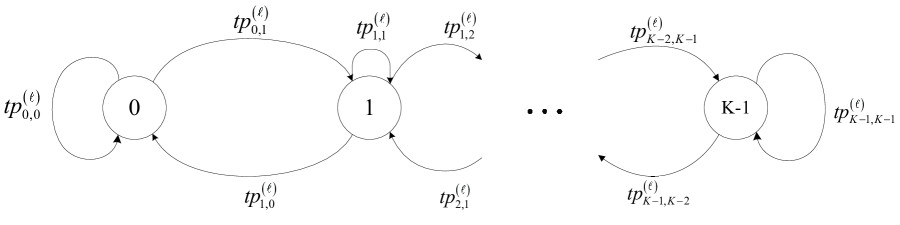
Figure 2: Illustration of $K$-state Markov chain

where $\sum\limits_{j=0}^{K-1}{tp_{ij}^{\left(\ell\right)}}=1$ and $\sum\limits_{i=0}^{K-1}{\pi_{i}^{\left(\ell\right)}}=1$. Fig. 2 shows the assumed $K$-state Markov chain for the $\ell$-th channel. Rayleigh distribution is a conventional model for the received signal envelop in a typical multipath propagation channel. It can be shown that the received SU’s SNR is proportional to the square of the signal envelop and exponentially distributed with the following probability density function [18] and [19],

$$p\left({{\gamma_{s}}}\right)=\frac{1}{{\overline{{\gamma_{s}}}}}\exp\left({-\frac{{{\gamma_{s}}}}{{\overline{{\gamma_{s}}}}}}\right)$$ (24)

where $\overline{{\gamma_{s}}}$ is both the mean and standard deviation of the SU’s SNR. Let $0=\gamma_{s,\ell}^{\left(0\right)}<\gamma_{s,\ell}^{\left(1\right)}<\cdots<\gamma_{s,\ell}^{\left({K-1}\right)}=\infty$ be the quantized SNR levels for the $\ell$-th channel. The channel will be in the state ${s_{m}^{\left(\ell\right)}}$, if the received SNR is placed within the interval of $\left[{\left.{\gamma_{s,\ell}^{\left(m\right)},\gamma_{s,\ell}^{\left({m+1}\right)}}\right)}\right.$. Considering (24) the steady-state probability of each state can be computed as,

$$\pi_{m}^{\left(\ell\right)}=\int_{\gamma_{s,\ell}^{\left(m\right)}}^{\gamma_{s,\ell}^{\left({m+1}\right)}}{\frac{1}{{\overline{{\gamma_{s,\ell}}}}}\exp\left({-\frac{x}{{\overline{{\gamma_{s,\ell}}}}}}\right)dx}$$ (25)

The transition probabilities can be calculated as [18], [19]

$$tp_{m,m+1}^{\left(\ell\right)}\approx\frac{{N_{m+1}^{\left(\ell\right)}T}}{{\pi_{m}^{\left(\ell\right)}}}{\rm{~{}}},{\rm{~{}~{}}}m=0,1,\ldots,K-2$$ (26)

and

$$tp_{m,m-1}^{\left(\ell\right)}\approx\frac{{N_{m}^{\left(\ell\right)}T}}{{\pi_{m}^{\left(\ell\right)}}}{\rm{~{}}},{\rm{~{}}}m=1,2,\ldots,K-1$$ (27)

where

$$N_{m}^{\left(\ell\right)}=\sqrt{\frac{{2\pi\gamma_{s,\ell}^{\left(m\right)}}}{{\overline{{\gamma_{s,\ell}}}}}}{f_{d}}\exp\left({-\frac{{\gamma_{s,\ell}^{\left(m\right)}}}{{\overline{{\gamma_{s,\ell}}}}}}\right)$$ (28)

where $N_{m}$ denotes the level crossing rate, and $f_{d}$ represents the maximum Doppler frequency, which can be calculated by knowing the moving speed of the mobile terminal, the speed of the light, and the carrier frequency. Other transition probabilities are given by,

$$tp_{m,m}^{\left(\ell\right)}=\left\{{\begin{array}[]{*{20}{c}}{1-tp_{m,m+1}^{\left(\ell\right)}{\rm{~{}}},\hfill}&{if{\rm{~{}}}m=0\hfill}\\ {1-tp_{m,m-1}^{\left(\ell\right)}{\rm{~{}}},\hfill}&{if{\rm{~{}}}m=K-1\hfill}\\ {1-tp_{m,m-1}^{\left(\ell\right)}-tp_{m,m+1}^{\left(\ell\right)}{\rm{~{}}},\hfill}&{O.W.\hfill}\\ \end{array}}\right.$$ (29)

The expected throughput in the next $s$ slots for the $\ell$-th channel can be computed as,

$$\begin{array}[]{c}E\left\{R\right\}_{s}^{\left(\ell\right)}=\underbrace{\Pr\left\{{S_{1}^{\left(\ell\right)}=s_{0}^{\left(\ell\right)}}\right\}r_{0}^{\left(\ell\right)}+\Pr\left\{{S_{1}^{\left(\ell\right)}=s_{1}^{\left(\ell\right)}}\right\}r_{1}^{\left(\ell\right)}+\cdots+\Pr\left\{{S_{1}^{\left(\ell\right)}=s_{K-1}^{\left(\ell\right)}}\right\}r_{K-1}^{\left(\ell\right)}}_{{\rm{1-th~{}next~{}time~{}slot}}}+\\ \underbrace{\Pr\left\{{S_{2}^{\left(\ell\right)}=s_{0}^{\left(\ell\right)}}\right\}r_{0}^{\left(\ell\right)}+\Pr\left\{{S_{2}^{\left(\ell\right)}=s_{1}^{\left(\ell\right)}}\right\}r_{1}^{\left(\ell\right)}+\cdots+\Pr\left\{{S_{2}^{\left(\ell\right)}=s_{K-1}^{\left(\ell\right)}}\right\}r_{K-1}^{\left(\ell\right)}}_{{\rm{2-th~{}next~{}time~{}slot}}}+\\ \vdots\\ \underbrace{\Pr\left\{{S_{s}^{\left(\ell\right)}=s_{0}^{\left(\ell\right)}}\right\}r_{0}^{\left(\ell\right)}+\Pr\left\{{S_{s}^{\left(\ell\right)}=s_{1}^{\left(\ell\right)}}\right\}r_{1}^{\left(\ell\right)}+\cdots+\Pr\left\{{S_{s}^{\left(\ell\right)}=s_{K-1}^{\left(\ell\right)}}\right\}r_{K-1}^{\left(\ell\right)}}_{{\rm{s-th~{}next~{}time~{}slot}}}\\ \end{array}$$ (30)

where ${r_{i}^{\left(\ell\right)}}$ denotes the transmission rate in the $i$-th state of the $\ell$-th channel due to exploited adaptive modulation coding scheme, and $\Pr\left\{{S_{j}^{\left(\ell\right)}=s_{i}^{\left(\ell\right)}}\right\}=\pi_{i}^{\left(\ell\right)}$ for all $1\leq j\leq s{\rm{~{}}},0\leq i\leq K-1$. So we can simplify (30) as,

$$E\left\{R\right\}_{s}^{\left(\ell\right)}=s\left({\pi_{0}^{\left(\ell\right)}r_{0}^{\left(\ell\right)}+\pi_{1}^{\left(\ell\right)}r_{1}^{\left(\ell\right)}+\cdots+\pi_{K-1}^{\left(\ell\right)}r_{K-1}^{\left(\ell\right)}}\right)$$ (31)

We define run as a consecutive series of idle states without occupied states. Hence, a run is a period within a SU could use the resource.

$$\Pr\left[{{\rm{run~{}length~{}}}\geq{\rm{~{}}}s}\right]={\left({1-{P_{\ell,00}}}\right)^{s-1}}$$ (32)

Let ${AP_{\ell,s}}$ be the absence probability of the $\ell$-th PU in the next $s$ consecutive time-slot. Considering (32), we have,

$${AP_{\ell,s}}={P_{\ell,0}}\times\Pr\left[{{\rm{run~{}length~{}}}\geq{\rm{~{}}}s}\right]={P_{\ell,0}}{\left({1-{P_{\ell,00}}}\right)^{s-1}}$$ (33)

When the SU needs to perform the HO procedure, it assigns a weight to each channel. Considering (31) and (33), the SU assigns weight ${w_{\ell}}$ to the $\ell$-th channel using the following formula:

$${w_{\ell}}=\frac{{E\left\{R\right\}_{s}^{\left(\ell\right)}}}{{{AP_{\ell,s}}}}$$ (34)

Then the SU sorts the channels based on their weights, decreasingly and starts to sense the channels using the derived sensing sequence. As a result, arranging spectrums by their weights gives an opportunity to the SU to sense spectrums that are more likely idle as well as higher expected throughput. Obviously, we expect that the overall achievable throughput in the WBHO scheme is higher than the SMHO approach.

V Simulation Results

In this section, we first evaluate the performance of the SMHO scheme by an exhaustive set of simulations to demonstrate the effect of different parameters introduced throughout the paper. We then consider the performance of the WBHO scheme and compare the result with that of the SMHO scheme. To set up a simulation environment, the values of SNR and sampling frequency are adopted from [11], $P_{d}^{\min}$ and $P_{fa}^{\max}$ are chosen according to IEEE 802.22 [17]. These values are given in Table. I.

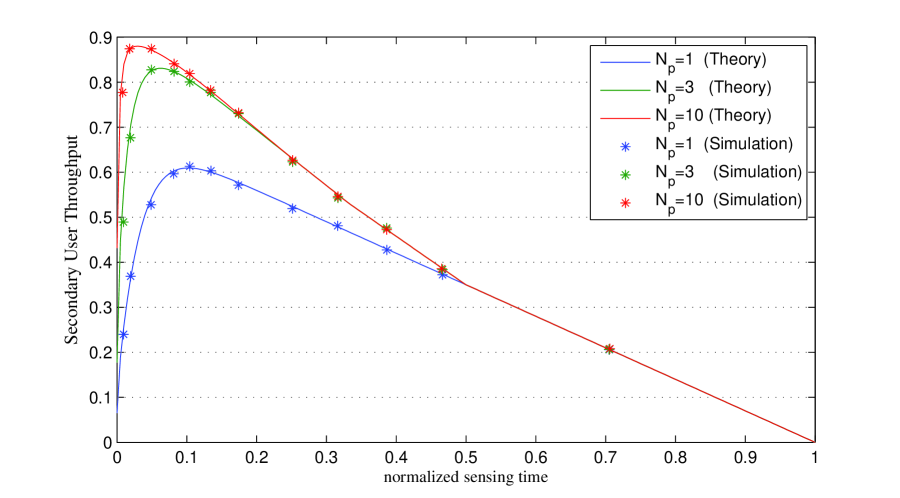
Figure 3: The average rate versus $\frac{\tau}{T}$ for various amount of $N_{p}$

The probabilities of the PUs’ presence, i.e, ${P_{k,0}}~{}~{}{\rm{}}\forall 1\leq k\leq{N_{p}}$, are assumed to be identical and equal to $0.65$. The average throughput has been computed after simulating the scenario for $1200$ time-slots. Fig. 3 verifies our analysis and illustrates the plots of achievable rate of the SMHO versus the sensing time $\tau$ normalized to slot period for different number of $N_{p}$ (the number of the PUs). For a large sensing time $\tau$, the plots for different values of $N_{p}$ coincide.

This behavior is expected due to our previous discussions on the constraints which affect the number of possible HOs for a SU. As stated in (12), the number of possible HOs is dictated by two factors; namely, the number of primary channels $N_{p}$, and the ratio $\left(T-\tau\right)/\left(\tau+\tau_{ho}\right)$. Therefore, as $\tau$ increases in Fig. 3, we observe that the second factor dominates and regardless of the number of available primary channels $N_{p}$, the achieved throughput becomes limited to a value corresponding to a lower $N_{p}$. The observed coincidences of the plots in Fig. 3 demonstrate this effect. The rate of the SU where there are $10$ primary channels equals the rate of the SU with $3$ primary channels for approximately $\tau>1/4T$. Similarly, the rate achieved by a SU with $3$ primary channels is equal to the rate of a SU with only $1$ primary channel. Other important observations can be made through Fig. 3. First, since all the curves posses a maxima, there exists an optimum value for the spectrum sensing time. Second, as the number of primary channels increases, the SU throughput increases as well, but in a saturating manner.

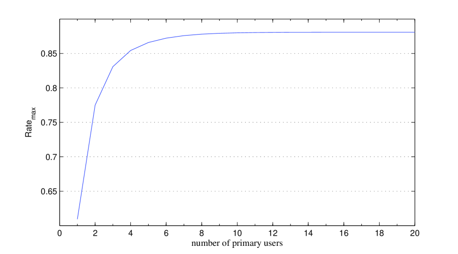
Figure 4: The maximum rate versus the number of primary users

Fig. 4 verifies the Proposition and demonstrates the plot of maximum possible achievable rate (obtained by the optimum value of sensing time which is seen for the $N_{p}=1,~{}3,~{}10$ in the Fig. 3) versus $N_{p}$. When $N_{p}$ increases, the overall rate increases as well. On the other hand, increasing in the value of $N_{p}$ leads to increment of the average number of HOs, and as the number of HOs increases, the transmission time reduces, so the maximum rate saturates.

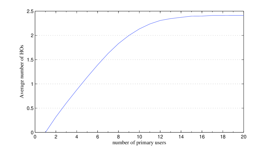
Figure 5: The average number of HOs versus the number of primary users

Fig. 5 illustrates the plot of average number of handover versus $N_{p}$. From this Fig. we can see that as the number of available channels increases, the average number of HOs in order to find an idle channel, increases. That is, by the increment of $N_{p}$, $\alpha$ in (12) increases, and ${\overline{g}_{SMHO}}$ in (11) increases, consequently. However, as we see in our further simulation, it does not lead to higher throughput.

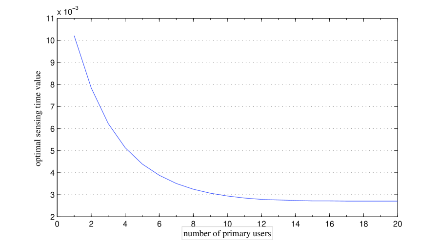
Figure 6: The optimum value for $\tau$ versus $N_{p}$

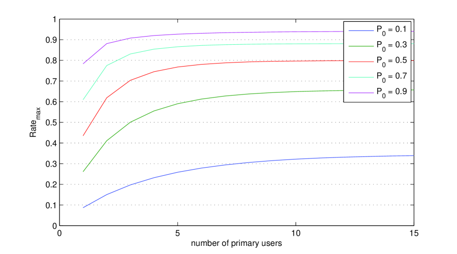
Figure 7: Maximum achievable rate versus $N_{p}$ for different values of $P_{0}$

Fig. 6 indicates that when $N_{p}$ increases the value of $\tau_{opt}$, in which the maximum rate is achieved, decreases; because the higher probability of finding idle spectrum is more important than the sensing accuracy, as there are many spectrums that the SU can utilize them with no priority. However, when ${N_{P}}\geq\left\lfloor{\frac{{T-{\tau_{\min}}}}{{{\tau_{\min}}+{\tau_{ho}}}}}\right\rfloor+1$, by the increase of $N_{p}$, the optimal value of sensing time, i.e., $\tau_{opt}$ and consequently the maximum achievable rate will not change, for the same reason explained in the Proposition. In Fig. 7 the effect of PU’s absence probability $(P_{0})$ on the achievable rate is shown. The increase of $P_{0}$ increases the chance of finding a transmission opportunity and improves the SU’s throughput, as well.

In the following, we evaluate the performance of the WBHO scheme and its advantages compared to the SMHO approach.

In order to simulate the WBHO scheme, the state transition probability of each PU (in the ON-OFF model) is assumed to be a uniform random variable within $0.1$ and $0.9$. Channel is modelled via $11$-state Markov process using the same parameter as Table I in [19]. At the end of each time-slot for the current channel, the SU calculates the $p$ in which $E_{i}\left(p\right)=3$ and compares it with $p_{0}=\%90$. The HO procedure is started provided that $p>p_{0}$. In this case, the SU establishes a sorted set of the channels based on the weighted computed in (34) for $s=5$ time-slot, and then starts to sense the channels in order. For the SHMO scheme, the same process has been performed, but the SU sorts channels based on their numbers, sequentially. The average throughput is obtained after $1200$ tim slots simulation.

Fig. 8 shows the plot of the SU’s average achievable throughput of the both schemes versus the sensing time. This figure is noticeable in twofold: First, the results indicate the better performance of the WBHO schemes. In fact, regardless of the case $N_{p}=1$, where two schemes offer the same throughput, the SU can achieve higher average throughput by applying the WBHO schemes for selecting its sensing sequence. Second, unlike the SMHO, the throughput of the SU for different number of PUs is not coincide; because having more PUs offers more spectrum bands with different conditions which improves the chance of having a channel with higher expected throughput, which depends on the PU absence probability and the channel gain. While for $\tau>0.5T$, regardless of the number of PUs, we cannot run the HO procedure and sense more than one channel (see (12)), however, we achieve a higher throughput by the increase of $N_{p}$ as a result of having a higher probability to find a channel with a more proper conditions. Finally, Fig. 9 represents the average number of HOs versus sensing time for various number of the PUs. Raising the number of the PUs leads to the increment of the number of HOs required to find a transmission opportunity. Moreover, average number of HOs reduces if the SU assigns more time to sense a channel due constraint imposed by (11). It is worth mentioning that the average number of HOs for the WBHO scheme is lower than the SMHO for all values of sensing time and the number of the PUs. Therefore, the SU can achieve higher average throughput with lower HOs and equivalently less consumed energy.

VI Conclusion

In this paper, we have considered the cognitive access of primary channels by a secondary user. The average detection time by the secondary user using SMHO and WBHO schemes have been evaluated. We have formulated an optimization problem in order to find the optimum sensing time in which the maximum throughput can be achieved. The tradeoff between the maximum achievable throughput and the consumed energy has been investigated. Finally, we have introduced a design parameter to modify our optimization problem addressing this tradeoff. Due to the new optimization problem, the acceptable throughput can be achieved while the energy consumption is more reasonable.

Before proofing Lemma 3, we note that if the SU transmits on the $(m+1)$-th channel (i.e., after $m$ times handover), the maximum rate in the slot is calculated as

$${r^{\left(m\right)}}={C_{0}}{P_{m+1,0}}\left({1-\frac{{ET_{m}}}{T}}\right)\left({1-{P_{fa}}\left(\tau\right)}\right)+{C_{1}}{P_{m+1,1}}\left({1-\frac{{ET_{m}}}{T}}\right)\left({1-{P_{d}}\left(\tau\right)}\right)$$ (35)

$$ET_{m}=\tau+m\left({\tau+{\tau_{ho}}}\right)$$ (36)

where $ET_{m}$ is the time spent until the SU chooses $(m+1)$-th spectrum for the transmission.

Now, we prove the lemma using the mathematical induction. Let ${R^{\left({k}\right)}}$ denote the average normalized rate when the maximum number of allowable HOs is $k$. We intend to show that $R^{\left(k\right)}$ can be calculated as

$$R^{\left(k\right)}=\sum\limits_{m=0}^{k}{\left({{C_{1}}{P_{m+1,1}}\left({1-{P_{d}}}\right)+{C_{0}}{P_{m+1,0}}\left({1-{P_{fa}}}\right)}\right){q_{0}}{q_{1}}\cdots{q_{m}}\left({1-\frac{{\tau+m\left({\tau+{\tau_{ho}}}\right)}}{T}}\right)}$$ (37)

For $k=0$, the maximum achievable rate can be calculated as [11]

$${R^{(0)}}={C_{0}}{P_{0}}\left({1-\frac{\tau}{T}}\right)\left({1-{P_{fa}}\left(\tau\right)}\right)+{C_{1}}{P_{1}}\left({1-\frac{\tau}{T}}\right)\times\left({1-{P_{d}}\left(\tau\right)}\right)$$ (38)

Suppose ${R^{\left({k}\right)}}$ is true, we investigate the validity of ${R^{\left({k+1}\right)}}$. We know,

$${R^{\left({k+1}\right)}}={R^{\left(k\right)}}+{r^{\left({k+1}\right)}}\times\Pr\left\{{{\rm{SU~{}transmittsin}}{{(k+2)}^{th}}{\rm{channel}}}\right\}$$ (39)

where ${r^{\left(k+1\right)}}$ is defined in (35) and $\Pr\left\{{{\rm{SU~{}transmitts~{}in~{}}}{{(k+2)}^{th}}{\rm{channel}}}\right\}$ is equal to $\Pr\left\{{{\rm{Number~{}of~{}HOs}}=k+1}\right\}$, where based on independency of different channels, is equal to ${q_{1}}\times{q_{2}}\times\cdots\times{q_{k+1}}$ , where $q_{k}$ is defined as (10). Therefore,

$$\begin{array}[]{r}{R^{\left({k+1}\right)}}={R^{\left(k\right)}}+\left({{C_{1}}{P_{k+2,1}}\left({1-{P_{d}}}\right)+{C_{0}}{P_{k+2,0}}\left({1-{P_{fa}}}\right)}\right)\times\\ {q_{1}}{q_{2}}\cdots{q_{m}}\left({1-\frac{{\tau+\left({k+1}\right)\left({\tau+{\tau_{ho}}}\right)}}{T}}\right)\\ \end{array}$$ (40)

which leads to (13) for $k=\alpha$, i.e., ${R^{\left(k\right)}}={R^{\left(\alpha\right)}}=R$.

TABLE I: Simulation Parameters

$P_{d}^{\min}$	$P_{fa}^{\max}$	$f_{s}$ (MHz)	$\gamma$ (dB)	Noise Spectral density	$T$ (ms)	$\tau_{ho}$ (ms)	$N_{p}$	$\frac{{{C_{1}}}}{{{C_{0}}}}$
0.9	0.1	6	-20	-174 dBm/Hz	100	0.1	10	0.1

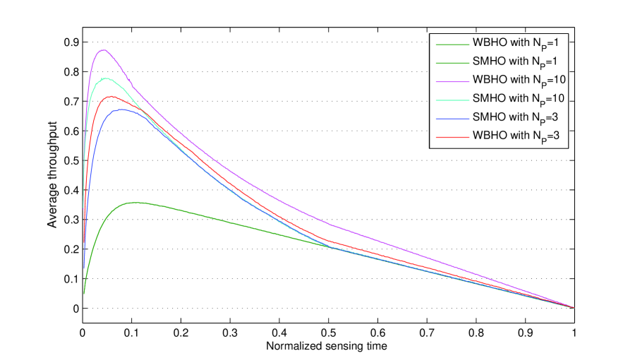
Figure 8: Comparison between the throughput of the SMHO and WBHO schemes for various values of $N_{p}$

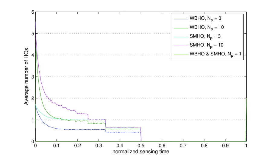
Figure 9: Comparison between the average number of HOs versus the sensing time for various number of $N_{p}$

References

- [1] I. F. Akyildiz, W. Y. Lee, M. C. Vuran, , and S. Mohanty, “Next generation / dynamic spectrum access / cognitive radio wireless networks: A survey,” Computer Networks Journal (Elsevier), vol. 50, pp. 2127–2159, Sept. 2006.
- [2] S. Haykin, “Cognitive radio: Brain-empowered wireless communications,” IEEE J. Sel. Areas Commun, vol. 23, no. 2, pp. 201–220, Feb. 2005.
- [3] L. C. Wang and A. Chen, “On the performance of spectrum handoff for link maintenance in cognitive radio,” in Proc. Int. Symp. Wireless Pervasive Comput., pp. 670–674, May 2008.
- [4] P. Paysarvi-Hoseini and N. C. Beaulieu, “Optimal wideband spectrum sensing framework for cognitive radio systems,” accepted for publication on IEEE Trans. Signal Process., 2011.
- [5] A. W. Min and K. G. Shin, “Exploiting multi-channel diversity in spectrum-agile networks,” IEEE International Conference on Computer Communications (INFOCOM), April 2008.
- [6] B. Hamdaoui, “Adaptive spectrum assessment for opportunistic access in cognitive radio networks,” IEEE Trans. on Wireless Commun., vol. 8, no. 2, pp. 922–930, Feb. 2009.
- [7] L. C. Wang, C. W. Wang, and F. Adachi, “Load-balancing spectrum decision for cognitive radio networks,” IEEE J. on Sel. Areas in Commun., vol. 29, no. 4, pp. 757–769, April 2011.
- [8] G. Chung, S. Vishwanath, and C. Hwang, “On the fundamental limits of interweaved cognitive radios,” preprint available at http://arxiv.org/PS cache/arxiv/pdf/0910/0910.1639v1.pdf, Oct. 2009.
- [9] X. Wang, “Joint sensing-channel selection and power control for cognitive radios,” IEEE Tarns. on Wireless Commun., vol. 10, no. 3, March 2011.
- [10] H. Kim and K. G. Shin, “Efficient discovery of spectrum opportunities with mac-layer sensing in cognitive radio networks,” IEEE Trans. on Wireless Commun., vol. 7, no. 5, pp. 533–545, May 2008.
- [11] Y. C. Liang, Y. Zeng, E. C. Y. Peh, and A. T. Hoang, “Sensing-throughput tradeoff for cognitive radio networks,” IEEE Trans. Wireless Communication, vol. 7, no. 4, pp. 1326–1337, Apr. 2008.
- [12] G. Yuan, R. C. Grammenos, Y. Yang, and W. Wang, “Performance analysis of selective opportunistic spectrum access with traffic prediction,” IEEE Tarns. on Veh. Technol., vol. 59, no. 4, pp. 1949–1959, May 2010.
- [13] D. J. Lee and M. S. Jang, “Optimal spectrum sensing time considering spectrum handoff due to false alarm in cognitive radio networks,” IEEE Comm. Letters, vol. 13, no. 12, pp. 899–901, December 2009.
- [14] R. Urgaonkar and M. Neely, “Opportunistic scheduling with reliability guarantees in cognitive radio networks,” IEEE Tarns. on Mobile Comput., vol. 8, no. 6, pp. 766–777, Jun. 2009.
- [15] T. Ycek and H. Arslan, “A survey of spectrum sensing algorithms for cognitive radio applications,” IEEE Commun. Surveys and Tutorials, vol. 11, no. 1, pp. 116–160, 2009.
- [16] H. Urkowitz, “Energy detection of unknown deterministic signals,” Proc. IEEE, vol. 55, pp. 523–531, Apr. 1967.
- [17] C. R. Stevenson, G. Chouinard, Z. Lei, W. Hu, and S. J. Shellhammer, “Ieee 802.22: The first cognitive radio wireless regional area network standard,” IEEE Comm. Mag., vol. 47, no. 1, pp. 130–138, Jan 2009.
- [18] H. S. Wang and N. Moayeri, “Finite-state markov channel - a useful model for radio communication channels,” IEEE Tarns. on Veh. Technol., vol. 44, no. 1, pp. 163–171, Feb. 1995.
- [19] Q. Zhang and S. A. Kassam, “Finite-state markov model for rayleigh fading channels,” IEEE Tarns. on Commun., vol. 47, no. 11, pp. 1688–1692, Nov. 1999.