Guaranteed violation of a Bell inequality without aligned reference frames or calibrated devices

Abstract

Bell tests—the experimental demonstration of a Bell inequality violation—are central to understanding the foundations of quantum mechanics, underpin quantum technologies, and are a powerful diagnostic tool for technological developments in these areas. To date, Bell tests have relied on careful calibration of the measurement devices and alignment of a shared reference frame between the two parties—both technically demanding tasks in general. Surprisingly, we show that neither of these operations are necessary, violating Bell inequalities with near certainty with (i) unaligned, but calibrated, measurement devices, and (ii) uncalibrated and unaligned devices. We demonstrate generic quantum nonlocality with randomly chosen local measurements on a singlet state of two photons implemented with reconfigurable integrated optical waveguide circuits based on voltage-controlled phase shifters. The observed results demonstrate the robustness of our schemes to imperfections and statistical noise. This new approach is likely to have important applications in both fundamental science and in quantum technologies, including device independent quantum key distribution.

Nonlocality is arguably among the most striking aspects of quantum mechanics, defying our intuition about space and time in a dramatic way bell . Although this feature was initially regarded as evidence of the incompleteness of the theory EPR , there is today overwhelming experimental evidence that nature is indeed nonlocal BellExp . Moreover, nonlocality plays a central role in quantum information science, where it proves to be a powerful resource, allowing, for instance, for the reduction of communication complexity CC and for device-independent information processing  DI ; randomness1 ; randomness2 ; rabelo .

In a quantum Bell test, two (or more) parties perform local measurements on an entangled quantum state, Fig. 1(a). After accumulating enough data, both parties can compute their joint statistics and assess the presence of nonlocality by checking for the violation of a Bell inequality. Although entanglement is necessary for obtaining nonlocality it is not sufficient. First, there exist some mixed entangled states that can provably not violate any Bell inequality since they admit a local model werner . Second, even for sufficiently entangled states, one needs judiciously chosen measurement settings Y.C.Liang:PRA:042103 . Thus although nonlocality reveals the presence of entanglement in a device-independent way, that is, irrespectively of the detailed functioning of the measurement devices, one generally considers carefully calibrated and aligned measuring devices in order to obtain a Bell inequality violation. This in general amounts to having the distant parties share a common reference frame and well calibrated devices. Although this assumption is typically made implicitly in theoretical works, establishing a common reference frame, as well as aligning and calibrating measurement devices in experimental situations are never trivial issues. It is therefore an interesting and important question whether such requirements can be dispensed with.

It was recently shown RandBIV:2010 that, for Bell tests performed in the absence of a shared reference frame, i.e., using randomly chosen measurement settings, the probability of obtaining quantum nonlocality can be significant. For instance, considering the simple Clauser-Horne-Shimony-Holt (CHSH) scenario CHSH , randomly chosen measurements on the singlet state lead to a violation of the CHSH inequality with probability of $\sim 28\%$; moreover this probability can be increased to $\sim 42\%$ by considering unbiased measurement bases. The generalization of these results to the multipartite case were considered in Refs. RandBIV:2010 ; RandBIV:2011 , as well as as schemes based on decoherence-free subspaces cabello . Although these works demonstrate that nonlocality can be a relatively common feature of entangled quantum states and random measurements, it is of fundamental interest and practical importance to establish whether Bell inequality violation can be ubiquitous.

Here we demonstrate that nonlocality is in fact a far more generic feature than previously thought, violating CHSH inequalities without a shared frame of reference, and even with uncalibrated devices, with near-certainty. We first show that whenever two parties perform three mutually unbiased (but randomly chosen) measurements on a maximally entangled qubit pair, they obtain a Bell inequality violation with certainty—a scheme that requires no common reference frame between the parties, but only a local calibration of each measuring device. We further show that when all measurements are chosen at random (i.e., calibration of the devices is not necessary anymore), although Bell violation is not obtained with certainty, the probability of obtaining nonlocality rapidly increases towards one as the number of different local measurements increases. We perform these random measurements on the singlet state of two photons using a reconfigurable integrated waveguide circuit, based on voltage-controlled phase shifters. The data confirm the near-unit probability of violating an inequality as well as the robustness of the scheme to experimental imperfections—in particular the non-unit visibility of the entangled state—and statistical uncertainty. These new schemes exhibit a surprising robustness of the observation of nonlocality that is likely to find important applications in diagnostics of quantum devices (e.g.. removing the need to calibrate the reconfigurable circuits used here) and quantum information protocols, including device independent quantum key distribution DI and other protocols based on quantum nonlocality randomness1 ; randomness2 ; rabelo and quantum steering onesided .

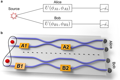
Figure 1: Bell violations with random measurements. (a) Schematic representation of a Bell test:. (b) Schematic of the integrated waveguide chip used to implement the new schemes described here. Alice and Bob’s measurement circuits consist of waveguides to encode photonic qubits, directional couplers that implement Hadamard-like operations, thermal phase shifters to implement arbitrary measurements and detectors.

Results

Bell test using random measurement triads. Two distant parties, Alice and Bob, share a Bell state. Here we will focus on the singlet state

$$\mbox{$|\Psi^{-}\rangle$}=\frac{1}{\sqrt{2}}\left(\mbox{$|0\rangle$}_{A}\mbox{$|1\rangle$}_{B}-\mbox{$|1\rangle$}_{A}\mbox{$|0\rangle$}_{B}\right),$$ (1)

though all our results can be adapted to hold for any two-qubit maximally entangled state. Let us consider a Bell scenario in which each party can perform 3 possible qubit measurements labeled by the Bloch vectors $\vec{a}_{x}$ and $\vec{b}_{y}$ ($x,y=1,2,3)$, and where each measurement gives outcomes $\pm 1$. After sufficiently many runs of the experiment, the average value of the product of the measurement outcomes, i.e. the correlators $E_{xy}=-\vec{a}_{x}\cdot\vec{b}_{y}$, can be estimated from the experimental data. In this scenario, it is known that all local measurement statistics must satisfy the CHSH inequalities:

$$\left|E_{xy}+E_{xy^{\prime}}+E_{x^{\prime}y}-E_{x^{\prime}y^{\prime}}\right|\leq 2,$$ (2)

and their equivalent forms where the negative sign is permuted to the other terms and for different pairs $x,x^{\prime}$ and $y,y^{\prime}$; there are, in total, 36 such inequalities.

Interestingly, it turns out that whenever the measurement settings are unbiased, i.e. $\vec{a}_{x}\cdot\vec{a}_{x^{\prime}}=\delta_{x,x^{\prime}}$ and $\vec{b}_{y}\cdot\vec{b}_{y^{\prime}}=\delta_{y,y^{\prime}}$, then at least one of the above CHSH inequalities must be violated — except for the case where the orthogonal triads (from now on simply referred to as triads) are perfectly aligned, i.e. for each $x$, there is a $y$ such that $\vec{a}_{x}=\pm\vec{b}_{y}$. Therefore, a generic random choice of unbiased measurement settings — where the probability that Alice and Bob’s settings are perfectly aligned is zero (for instance if they share no common reference frame) — will always lead to the violation of a CHSH inequality.

Proof. Assume that $\{\vec{a}_{x}\}$ and $\{\vec{b}_{y}\}$ are orthonormal bases. Since the correlators of the singlet state have the simple scalar product form $E_{xy}=-\vec{a}_{x}\cdot\vec{b}_{y}$, the matrix

$${\cal E}=\left(\begin{array}[]{ccc}E_{11}&E_{12}&E_{13}\\ E_{21}&E_{22}&E_{23}\\ E_{31}&E_{32}&E_{33}\end{array}\right)$$ (6)

contains (in each column) the coordinates of the three vectors $-\vec{b}_{y}$, written in the basis $\{\vec{a}_{x}\}$.

By possibly permuting rows and/or columns, and by possibly changing their signs (which corresponds to relabeling Alice and Bob’s settings and outcomes), we can assume, without loss of generality, that $E_{11},E_{22}>0$ and that $E_{33}>0$ is the largest element (in absolute value) in the matrix ${\cal E}$. Noting that $\vec{b}_{3}=\pm\vec{b}_{1}\times\vec{b}_{2}$ and therefore $|E_{33}|=|E_{11}E_{22}-E_{12}E_{21}|$, these assumptions actually imply $E_{33}=E_{11}E_{22}-E_{12}E_{21}\geq E_{11},E_{22},|E_{12}|,|E_{21}|$ and $E_{12}E_{21}\leq 0$; we will assume that $E_{12}\leq 0$ and $E_{21}\geq 0$ (one can multiply both the $x=2$ row and the $y=2$ column by -1 if this is not the case).

With these assumptions, $(E_{11}+E_{21})\max[-E_{12},E_{22}]\geq E_{11}E_{22}-E_{12}E_{21}=E_{33}\geq\max[-E_{12},E_{22}]$, and by dividing by $\max[-E_{12},E_{22}]>0$, we get $E_{11}+E_{21}\geq 1$. One can show in a similar way that $-E_{12}+E_{22}\geq 1$. Adding these last two inequalities, we obtain

$$E_{11}+E_{21}-E_{12}+E_{22}\geq 2\,.$$ (7)

Since ${\cal E}$ is an orthogonal matrix, one can check that equality is obtained above (which requires that both $E_{11}+E_{21}=1$ and $-E_{12}+E_{22}=1$) if and only if $\vec{a}_{1}=\vec{b}_{1}$, $\vec{a}_{2}=\vec{b}_{2}$ and $\vec{a}_{3}=\vec{b}_{3}$. Therefore, if the two sets of mutually unbiased measurement settings $\{\vec{a}_{x}\}$ and $\{\vec{b}_{y}\}$ are not aligned, then inequality (7) is strict: a CHSH inequality is violated. Numerical evidence suggests that the above construction always gives the largest CHSH violation obtainable from the correlations (6). $\hfill\blacksquare$

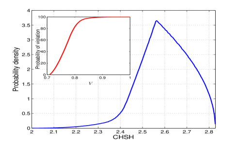
Figure 2: Bell tests using random measurement triads (theory). Distribution of the (maximum) CHSH violations for uniformly random measurement triads on a singlet state. The inset shows the probability of obtaining a CHSH violation as a function of the visibility $V$ of the Werner state; this probability is obtained by integrating the distribution of CHSH violations (main graph) over the interval $[2/V,2\sqrt{2}]$.

While the above result shows that a random choice of measurement triads will lead to nonlocality with certainty, we still need to know how these CHSH violations are distributed; that is, whether the typical violations will be rather small or large. This is crucial especially for experimental implementations, since in practice, various sources of imperfections will reduce the strength of the observed correlations. Here we consider two main sources of imperfections: limited visibility of the entangled state, and finite statistics.

First, the preparation of a pure singlet state is impossible experimentally and it is thus desirable to understand the effect of depolarizing noise, giving rise to a reduced visibility $V$:

$$\mbox{$|\Psi^{-}\rangle$}\rightarrow\rho_{V}=V\mbox{$|\Psi^{-}\rangle\!\langle\Psi^{-}|$}+(1-V)\frac{\mathbf{1}}{4}.$$ (8)

This, in turn, results in the decrease of the strength of correlations by a factor $V$. In particular, when $V\leq 1/\sqrt{2}$, the state (8) ceases to violate the CHSH inequality. States $\rho_{V}$ are known as Werner states werner .

Second, in any experiment the correlations are estimated from a finite set of data, resulting in an experimental uncertainty. To take into account this finite-size effect, we will consider a shifted classical bound $\mathcal{S}\geq 2$ of the CHSH expression (2) such that an observed correlation is only considered to give a conclusive demonstration of nonlocality if $\text{CHSH}>\mathcal{S}$. Thus, if the CHSH value is estimated experimentally up to a precision of $\delta$, then considering a shifted classical bound of $\mathcal{S}=2+\delta$ ensures that only statistically significant Bell violations are considered.

We have estimated numerically the distribution of the CHSH violations (the maximum of the left-hand-side of (2) over all $x,x^{\prime},y,y^{\prime}$) for uniformly random measurement triads on the singlet state (see Fig. 2). Interestingly, typical violations are quite large; the average CHSH value is $\sim 2.6$, while only $\sim 0.3\%$ of the violations are below $2.2$. Thus this phenomenon of generic nonlocality is very robust against the effect of finite statistics and of limited visibility, even in the case where both are combined. For instance, even after raising the cutoff to $\mathcal{S}=2.1$ and decreasing the singlet visibility to $V=0.9$, our numerical simulation shows that the probability of violation is still greater than 98.2% (see Fig 2).

Bell tests using completely random measurements. Although performing unbiased measurements does not require the spatially separated parties to share a common reference frame, it still requires each party to have good control of the local measurement device. Clearly, local alignment errors (that is, if the measurements are not exactly unbiased) will reduce the probability of obtaining nonlocality. In practice the difficulty of correctly aligning the local measurement settings depends on the type of encoding that is used. For instance, using the polarization of photons, it is rather simple to generate locally a measurement triad, using wave-plates. However, for other types of encoding, generating unbiased measurements might be much more complicated (see experimental part below).

This leads us to investigate next the case where all measurement directions $\{\vec{a}_{x},\vec{b}_{y}\}$ are chosen randomly and independently. For simplicity, we will focus here on the case where all measurements are chosen according to a uniform distribution on the Bloch sphere. Although this represents a particular choice of distribution, we believe that most random distributions that will naturally arise in an experiment will lead to qualitatively similar results, as indicated by our experimental results.

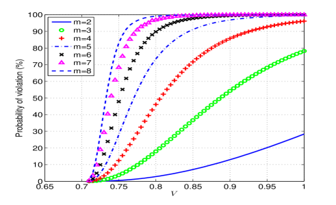
Figure 3: Bell tests using completely random measurements (theory). Plot of the probability of Bell violation as a function of the visibility $V$ of the Werner state, for different numbers $m$ of (completely random) measurements per party.

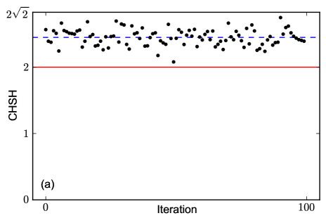
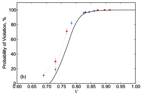
Figure 4: Bell tests requiring no shared reference frame. Here we perform Bell tests on a two-qubit Bell state, using randomly chosen measurement triads. Thus our experiment requires effectively no common reference frame between Alice and Bob. (a) 100 successive Bell tests; in each iteration, both Alice and Bob use a randomly-chosen measurement triad. For each iteration, the maximal CHSH value is plotted (black points). In all iterations, we get a CHSH violation; the red line indicates the local bound (CHSH=2). The smallest CHSH value is $\sim 2.1$, while the mean CHSH value (dashed line) is $\sim 2.45$. This leads to an estimate of the visibility of $V=\frac{2.45}{2.6}\simeq 0.942$, to be compared with $0.913\pm 0.004$ obtained by maximum likelihood quantum state tomography maxlike . This slight discrepancy is due to the fact that our entangled state is not exactly of the form of a Werner state. Error bars, which are too small to draw, were estimated using a Monte Carlo technique, assuming Poissonian photon statistics. (b) The experiment of (a) is repeated for Bell states with reduced visibility, illustrating the robustness of the scheme. Each point shows the probability of CHSH violation estimated using 100 trials. Uncertainty in probability is estimated as the standard error. Visibility for each point is estimated by maximum-likelihood quantum state tomography, where the error bar is calculated using a Monte Carlo approach, again assuming Poissonian statistics. Red points show data corrected for accidental coincidences (see Methods), the corresponding uncorrected data is shown in blue. Again, since our state is not exactly of the Werner form, we get slightly higher probabilities of CHSH violation than expected.

We thus now consider a Bell test in which Alice and Bob share a singlet, and each party can use $m$ possible measurement settings, all chosen randomly and uniformly on the Bloch sphere. We estimated numerically the probability of getting a Bell violation as a function of the visibility $V$ [of the state (8)] for $m=2,\ldots,8$; see Fig. 3. Note that for $m\geq 4$, additional Bell inequalities appear gisin ; we have checked however, that ignoring these inequalities and considering only CHSH leads to the same results up to a very good approximation. Fig. 3 clearly shows that the chance of finding a nonlocal correlation rapidly increases with the number of settings $m$. Intuitively, this is because when choosing an increasing number of measurements at random, the probability that at least one set of four measurements (2 for Alice and 2 for Bob) violates the CHSH inequality increases rapidly. For example, with $m=3$ settings, this probability is $78.2\%$ but with $m=4$, it is already 96.2%, and for $m=5$ it becomes 99.5%. Also, as with the case of unbiased measurements, the probability of violation turns out to be highly robust against depolarizing noise; for instance, for $V=0.9$ and $m\geq 5$, there is still at least 96.9% chance of finding a subset $\{\vec{a}_{x},\vec{a}_{x^{\prime}},\vec{b}_{y},\vec{b}_{y^{\prime}}\}$ among our randomly chosen measurements that gives nonlocal correlations.

Measurement devices. We use the device shown in Fig. 1(b) to implement Alice and Bob’s random measurements on an entangled state of two photons. The path encoded singlet state is generated from two unentangled photons using an integrated waveguide implementation politi1 ; politi2 of a nondeterministic cnot gate cnot1 ; cnot2 ; cnot3 to enable deliberate introduction of mixture. This state is then shared between Alice and Bob who each have a Mach-Zehnder (MZ) interferometer, consisting of two directional couplers (equivalent to beamsplitters) and variable phase shifters ($A_{1,2}$ and $B_{1,2}$) and single photon detectors. This enables Alice and Bob to independently make a projective measurement in any basis by setting their phase shifters to the required values matthews ; pete . The effect of the first phase-shifter is a rotation around the $Z$ axis of the Bloch sphere ($R_{Z}(\phi_{1})=e^{-i\phi_{1}\sigma_{Z}/2}$); since each directional coupler implements a Hadamard-like operation ($H^{\prime}=e^{i\pi/2}e^{-i\pi\sigma_{Z}/4}He^{-i\pi\sigma_{Z}/4}$, where $H$ is the usual Hadamard gate), the effect of the second phase shifter is a rotation around the $Y$ axis ($R_{Y}(\phi_{2})=e^{-i\phi_{2}\sigma_{Y}/2}$). Overall the MZ interferometer and phase shifters implement the unitary transformation $U(\phi_{1},\phi_{2})=R_{Y}(\phi_{2})R_{Z}(\phi_{1})$, which enables projective measurement in any qubit basis when combined with a final measurement in the logical ($Z$) basis using avalanche photodiode single photon detectors (APDs).

Each thermal phase shifter is implemented as a resistive element, lithographically patterned onto the surface of the waveguide cladding. Applying a voltage $v$ to the heater has the effect of locally heating the waveguide, thereby inducing a small change in refractive index $n$ ($dn/dT\approx 1\times 10^{-5}K$) which manifests as a phase shift in the MZ interferometer. There is a nonlinear relationship between the voltage applied and the resulting phase shift $\phi(v)$, which is generally well approximated by a quadratic relation of the form

$$\phi(v)=\alpha+\beta v^{2}.$$ (9)

In general, each heater must be characterized individually, i.e. by estimating the function $\phi(v)$. This is achieved by measuring single-photon interference fringes from each heater. The parameter $\alpha$ can take any value between 0 and $2\pi$ depending on the fabrication of the heater, while typically $\beta\sim 0.15\frac{\text{rad}}{V^{2}}$ matthews ; pete . For any desired phase, the corrected voltage can then be determined. This operation is necessary both for state tomography, and for implementing random measurement triads. In contrast, this calibration can be dispensed with when implementing completely random measurements. Indeed this represents the central point of this experiment, which requires no a priori calibration of the devices. Thus, In this case we simply choose random voltages from a uniform distribution, in the range $[0\text{V},7\text{V}]$, which is adequate to address phases in the range $0\leq\phi\leq 2\pi$—i.e. no a priori calibration of Alice and Bob’s devices is necessary.

Experimental violations with random measurement triads. We first investigate the situation in which Alice and Bob both use 3 orthogonal measurements. We generate randomly chosen measurement triads using a pseudo-random number generator. Having calibrated the phase/voltage relationship of the phase shifters, we then apply the corresponding voltages on the chip. For each pair of measurement settings, the coincidence counts between all of the 4 pairs of APDs are then measured for a fixed amount of time—the typical number of simultaneous photon detection coincidences is $\sim 1$ kHz. From these data we compute the maximal CHSH value as detailed above. This entire procedure is then repeated 100 times. The results are presented in Fig. 4a, where accidental coincidences, arising primarily from photons originating from different down-conversion events, which are measured throughout the experiment, have been subtracted from the data (the raw data, as well as more details on accidental events, can be found in the Methods). Remarkably, all 100 trials lead to a clear CHSH violation; the average CHSH value we observe is $\sim 2.45$, while the smallest measured value is $\sim 2.10$.

We next investigate the effect of decreasing the visibility of the singlet state: By deliberately introducing a temporal delay between the two photons arriving at the cnot gate, we can increase the degree of distinguishability between the two photons. Since the photonic cnot circuit relies on quantum interference HOM a finite degree of distinguishability between the photons results in this circuit implementing an incoherent mixture of the CNOT operation and the identity operation ob_prl . By gradually increasing the delay we can create states $\rho_{V}$ with decreasing visibilities. For each case, the protocol described above is repeated, which allows us to estimate the average CHSH value (over 100 trials). For each case we also estimate the visibility via maximum likelihood quantum state tomography. Figure 4b clearly demonstrates the robustness of our scheme, in good agreement with theoretical predictions: a considerable amount of mixture must be introduced in order to get an average CHSH value below 2.

Together these results show that large Bell violations can be obtained without a shared reference frame even in the presence of considerable mixture.

Experimental violations with completely random measurements. We now investigate the case where all measurements are chosen at random. The procedure is similar to the first experiment, but we now apply voltages chosen randomly from a uniform distribution, and independently for each measurement setting. Thus our experiment requires no calibration of the measurement MZ interferometers (i.e. the characterization of the phase-voltage relation), which is generally a cumbersome task. By increasing the number of measurements performed by each party ($m=2,3,4,5$), we obtain CHSH violations with a rapidly increasing probability, see Fig. 5. For $m=5$, we find 95 out of 100 trials lead to a CHSH violation. The visibility $V$ of the state used for this experiment was measured using state tomography to be $0.869\pm 0.003$, clearly demonstrating that robust violation of Bell inequalities is possible for completely random measurements.

It is interesting to note that the relation between the phase and the applied voltage is typically quadratic, see Eq. (9). Thus, by choosing voltages from a uniform distribution, the corresponding phase distribution is clearly biased. Our experimental results indicate that this bias has only a minor effect on the probability of obtaining nonlocality.

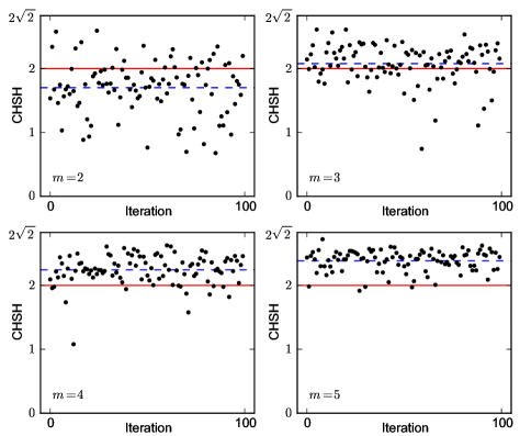
Figure 5: Experimental Bell tests using uncalibrated devices. We perform Bell tests on a two-qubit Bell state, using uncalibrated measurement interferometers, that is, using randomly-chosen voltages. For $m=2,3,4,5$ local measurement settings, we perform 100 trials (for each value of $m$). As the number of measurement settings $m$ increases, the probability of obtaining a Bell violation rapidly approaches one. For $m\geq 3$, the average CHSH value (dashed line) is above the local bound of CHSH=2 (red line). Error bars, which are too small to draw, were estimated by a Monte Carlo technique, assuming Poissonian statistics. Data has been corrected for accidentals (see Methods).

Discussion.

Bell tests provide one of the most important paths to gaining insight into the fundamental nature of quantum physics. The fact that they can be robustly realised without the need for a shared reference frame or calibrated devices promises to provide new fundamental insight. In the future it would be interesting to investigate these ideas in the context of other Bell tests, for instance considering other entangled states or in the multipartite situation (see joel for recent progress in this direction), as well as in the context of quantum reference frames review ; costa .

The ability to violate Bell inequalities with a completely uncalibrated device, as was demonstrated here, has important application for the technological development of quantum information science and technology: Bell violations provide an unambiguous signature of quantum operation and the ability to perform such diagnostics without the need to first perform cumbersome calibration of devices should enable a significant saving in all physical platforms. These ideas could be particularly helpful for the characterization of entanglement sources without the need for calibrated and aligned measurement devices.

Finally Bell violations underpin many quantum information protocols, and therefore, the ability to realise them with dramatically simplified device requirements holds considerable promise for simplifying the protocols themselves. For example, device independent quantum key distribution DI allows two parties to exchange a cryptographic key and, by checking for the violation of a Bell inequality, to guarantee its security without having a detailed knowledge of the devices used in the protocol. Such schemes, however, do typically require precise control of the apparatus in order to obtain a sufficiently large violation. In other words, although a Bell inequality violation is an assessment of entanglement that is device-independent, one usually needs carefully calibrated devices to obtain such a violation. The ability to violate Bell inequalities without these requirements could dramatically simplify these communication tasks. The implementation of protocols based on quantum steering onesided may also be simplified by removing calibration requirements.

Note added. While completing this manuscript, we became aware of an independent proof of our theoretical result on Bell tests with randomly chosen measurement triads, obtained by Wallman and Bartlett joel , after one of us mentioned numerical evidence of this result to them.

I Methods

Photon counting and accidentals. In our experiments, we postselect on successful operation of the linear-optical cnot gate by counting coincidence events, that is, by measuring the rate of coincidental detection of photon pairs. Single photons are first detected using silicon avalanche photodiodes (APDs). Coincidences are then counted using a Field-Programmable Gate Array (FPGA) with a time window of $\sim 5$ns. We refer to these coincidence events as $\{t_{0}^{A},t_{0}^{B}\}$.

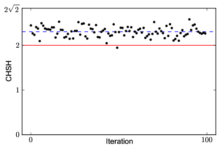
Figure 6: Raw data of experimental Bell tests requiring no shared reference frame. This figure shows the raw data, without correcting for accidental coincidences, of Fig. 4a. Here the average CHSH value is 2.30 (dashed line), leading to an estimate of the visibility of $V=\frac{2.3}{2.6}\simeq 0.885$, while the estimate from quantum state tomography is $V=0.861\pm 0.003$. Again, this discrepancy is due to the fact that our entangled state is not exactly of the form of a Werner state. Error bars, which are too small to draw, were estimated using a Monte-Carlo technique, assuming Poissonian photon statistics.

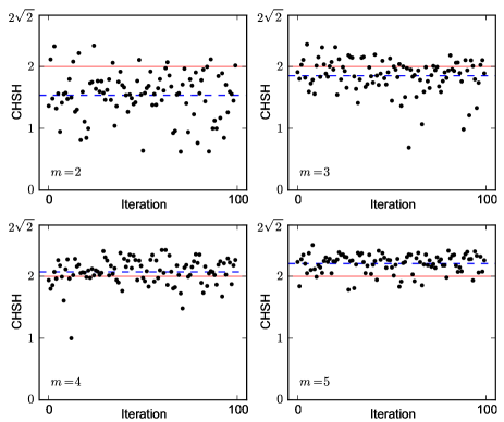
Figure 7: Raw data of experimental Bell tests using uncalibrated measurement interferometers (random voltages). This figure shows the raw data, without correcting for accidental coincidences, of Fig. 5. Error bars are estimated by a Monte Carlo technique, assuming Poissonian statistics. The visibility $V$ of the state used for this experiment was measured using state tomography to be $0.804\pm 0.003$.

Accidental coincidences have two main contributions: first, from photons originating from different down-conversion events arriving at the detectors within the time window; second, due to dark counts in the detectors. Here we directly measure the (dynamic) rate of accidental coincidences in real time, for the full duration of all the experiments described here. To do so, for each pair of detectors we measure a second coincidence count rate, namely $\{t_{0}^{A},t_{1}^{B}\}$, with $|t_{1}-t_{0}|=30\text{ns}$. In order to do this, we first split (duplicate) the electrical TTL pulse from each detector into two BNC cables. An electrical delay of 30ns is introduced into one channel, and coincidences (i.e. at $\{t_{0}^{A},t_{0}^{B}\}$) are then counted directly. Finally we obtain the corrected coincidence counts by subtracting coincidence counts at $\{t_{0}^{A},t_{1}^{B}\}$ from the raw coincidence counts at $\{t_{0}^{A},t_{0}^{B}\}$.

All experimental results presented in the main text have been corrected for accidentals. Here we provide the raw data. Fig 6 presents the raw data for Fig. 4(a) while Fig. 7 presents the raw data for Fig. 5. Notably, in Fig. 6, corresponding to the case of randomly chosen triads, all but one of the hundred trials feature a CHSH violation. The average violation is now $\sim 2.3$.

References

- (1) J. S. Bell, Physics (Long Island City, N.Y.) 1, 195 (1964).
- (2) A. Einstein, B. Podolsky, and N. Rosen, Phys. Rev. 47, 777 (1935).
- (3) A. Aspect, Nature 398, 189 (1999).
- (4) H. Buhrman, R. Cleve, S. Massar, and R. de Wolf, Rev. Mod. Phys. 82, 665 (2010).
- (5) A. Acín, N. Brunner, N. Gisin, S. Massar, S. Pironio, and V. Scarani, Phys. Rev. Lett. 98, 230501 (2007).
- (6) S. Pironio et al, Nature 464, 1021 (2010).
- (7) R. Colbeck and A. Kent, J. Phys. A 44, 095305 (2011).
- (8) R. Rabelo, M. Ho, D. Cavalcanti, N. Brunner, and V. Scarani, Phys. Rev. Lett. 107, 050502 (2011).
- (9) R.F. Werner, Phys. Rev. A 40, 4277 (1989).
- (10) Y.-C. Liang and A. C. Doherty, Phys. Rev. A 75, 042103 (2007).
- (11) Y.-C. Liang, N. Harrigan, S. D. Bartlett, and T. G. Rudolph, Phys. Rev. Lett. 104, 050401 (2010).
- (12) J. F. Clauser, M. A. Horne, A. Shimony and R. Holt, Phys. Rev. Lett. 23, 880 (1969).
- (13) J. J. Wallman, Y.-C. Liang, and S. D. Bartlett, Phys. Rev. A 83, 022110 (2011).
- (14) A. Cabello, Phys. Rev. Lett. 91, 230403 (2003).
- (15) C. Branciard, E.G. Cavalcanti, S.P. Walborn, V. Scarani, H.M. Wiseman, arXiv:1109.1435.
- (16) N. Gisin, arXiv:quant-ph/0702021.
- (17) A. Politi, M.J. Cryan, J.G. Rarity, S. Yu, and J.L. O’Brien, Science 320, 646 (2008).
- (18) A. Politi, J.C.F. Matthews, and J.L. O’Brien, Science 325, 1221 (2009).
- (19) T.C. Ralph, N.K. Langford, T.B. Bell, and A.G. White, Phys. Rev. A 65, 062324 (2002).
- (20) H.F. Hofmann and S. Takeuchi, Phys. Rev. A 66, 024308 (2002).
- (21) J.L. O’Brien, G.J. Pryde, A.G. White, T.C. Ralph and D. Branning, Nature 426, 264 (2003).
- (22) P.J. Shadbolt, M.R. Verde, A. Peruzzo, A. Politi, A. Laing, M. Lobino, J.C.F. Matthews, M.G. Thompson and J.L. O’Brien, arXiv:1108.3309.
- (23) J.C.F. Matthews, A. Politi, A. Stefanov, and J.L. O’Brien, Nature Photonics 3, 346 (2009).
- (24) C.K. Hong, Z.Y. Ou, and L. Mandel, Phys. Rev. Lett. 59, 2044 (1987).
- (25) J.L. O’Brien, G.J. Pryde, A. Gilchrist, D.F.V. James, N.K. Langford, T.C. Ralph, and A.G. White, Phys. Rev. Lett. 93, 080502 (2004).
- (26) D.F.V. James, P.G. Kwiat, W.J. Munro, and A.G. White, Phys. Rev. A 64, 052312 (2001).
- (27) J.J. Wallman and S.D. Bartlett, arXiv:1111.1864.
- (28) S.D. Bartlett, T. Rudolph and R.W. Spekkens, Rev. Mod. Phys. 79, 555 (2007).
- (29) F. Costa, N. Harrigan, T. Rudolph and C. Brukner, New J. Phys. 11 123007 (2009).
Acknowledgements.
We acknowledge useful discussions with Jonathan Allcock, Nicolas Gisin and Joel Wallman. We acknowledge financial support from the UK EPSRC, ERC, QUANTIP, PHORBITECH, Nokia, NSQI, the János Bolyai Grant of the Hungarian Academy of Sciences, the Swiss NCCR ”Quantum Photonics”, and the European ERC-AG QORE. J.L.O’B. acknowledges a Royal Society Wolfson Merit Award.I Methods