Estimation of scale functions to model heteroscedasticity by support vector machines
Abstract
A main goal of regression is to derive statistical conclusions on the conditional distribution of the output variable given the input values . Two of the most important characteristics of a single distribution are location and scale. Support vector machines (SVMs) are well established to estimate location functions like the conditional median or the conditional mean. We investigate the estimation of scale functions by SVMs when the conditional median is unknown, too. Estimation of scale functions is important e.g. to estimate the volatility in finance. We consider the median absolute deviation (MAD) and the interquantile range (IQR) as measures of scale. Our main result shows the consistency of MAD-type SVMs.
1 Introduction
Let be the distribution of a pair of random variables with values in a set where is an input variable and is a real-valued output variable. The goal in regression problems is to derive statistical conclusions on the conditional distribution of given . Generally, location and scale are considered as the two most important characteristics of a distribution and estimating these quantities is one of the main topics in statistics.
Regularized empirical risk minimization [26, 27, 18, 8] using the kernel trick proposed by [19] and the special case of support vector machines (SVMs) [26, 6, 18, 23] are well established methods in order to estimate the location of the conditional distribution of given . For an i.i.d. sample drawn from , the SVM-estimator is defined by
| (1) |
where is a loss function, is a certain space – a so-called reproducing kernel Hilbert space (RKHS) – of functions , and is a regularization parameter in order to prevent overfitting. We refer to [27, 18, 2, 8, 23] for the concept of an RKHS. There are a number of different quantities which describe the location of a single distribution and which can be estimated by SVMs by choosing a suitable loss function. The conditional mean function , can be estimated by using the least-squares loss and the -quantile function , , (see (2) below) by using the -pinball loss function
see [15, 14, 20, 25]. The choice leads to an estimate of the median function
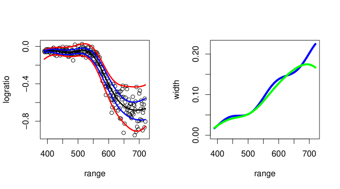
The goal of this paper is to investigate two methods to estimate the variability of the conditional distributions of given for via scale functions. Estimation of heteroscedasticity is interesting in many areas of applied statistics, e.g., for the estimation of volatility in finance. To fix ideas, let us illustrate what we mean by scale function estimation by considering a small data concerning the so-called LIDAR technique. LIDAR is the abbreviation of LIght Detection And Ranging. This technique uses the reflection of laser-emitted light to detect chemical compounds in the atmosphere. We consider the logarithm of the ratio of light received from two laser sources as the output variable , whereas the single input variable is the distance traveled before the light is reflected back to its source. We refer to [17] for more details on this data set. A scatterplot of the data set consisting of observations is shown in the left subplot of Figure 1 together with the fitted quantile curves based on SVMs using the pinball loss function for and the Gaussian RBF kernel for . By looking at the estimated median function (i.e., the black curve in the middle of the left subplot), we clearly see a nonlinear relationship between both variables which is almost constant for values of below and decreasing for higher values of range. However, there is also a considerable change of the variability of given : the variability is relatively small for small values of , but much larger for large values of . This becomes obvious by looking at the other estimated quantile curves in the left subplot or by looking at the right subplot of Figure 1 which shows the estimated width of intervals covering at least of the mass of . In this simple example we can just look onto the 2-dimensional plot to realize this kind of heteroscedasticity of the conditional distribution of given . However, this is obviously no longer possible if the input space is a high-dimensional Euclidean space or an abstract metric space. Hence an automatic and non-parametric method to model and to estimate such kind of variability becomes important.
Therefore, this article investigates how two classical scale quantities of the conditional distribution of given can be estimated by use of SVMs.
Such scale functions are quite common in a heteroscedastic model like , where denotes the location function and denotes the stochastic error term. Note, that we will not assume
such a specific model.
As in case of location, there are
several well established quantities which describe the scale, e.g., [10, Chap. 5]
the variance function:
, ,
the median absolute
deviation from the median (MAD) function:
,
the interquantile range (IQR) function for quantiles :
, .
Note that these three quantities are not directly comparable. However,
and times MAD
are both quantities for the width of an interval covering at least of the probability mass of
.
There is a vast literature on the estimation of scale functions, often based on special parametric dispersion models, see, e.g.,
[11, 21, 12],
and for a wavelet thresholding approach for univariate
regression models we refer to [3].
In this article, we consider the MAD function and the IQR function and show how both can be consistently estimated in a purely nonparametric manner with SVMs. In case of the MAD, we estimate the unknown median function by an SVM and calculate the estimated absolute residuals in a first step. In a second step, we estimate the conditional median of the absolute residuals by the SVM based on a smoothed version of the -pinball loss defined in (4) below for the pairs of random variables . The resulting estimator is called MAD-type SVM and it is shown in Subsection 2.1 that it is risk-consistent (up to any predefined ) even though (i) the estimation in the second step cannot be based on the true residuals but has to be based on the estimated residuals because the true median function is unknown and (ii) the random variables are not i.i.d. In case of the IQR , we respectively estimate the -quantile function by use of the -pinball loss so that we get as an estimate, which we call IQR-type SVM. As this is the difference of two standard SVMs, we can carry over many well-known facts on SVMs in this case in Subsection 2.2. In both cases, available software, e.g., the R-package kernlab [13] or the C++ implementation mySVM [16], can be used since we essentially have to calculate SVMs for pinball losses.
The rest of the paper has the following structure. Section 2 contains with Theorem 2.2 our main result. Section 3 contains not only the proof of this theorem, but also gives two new consistency results in the -sense for SVMs based on the pinball loss, see Lemma 3.1 and Theorem 3.2. Although we need these results in our proof of Theorem 2.2, we think that they are interesting in its own, because they improve earlier consistency results of SVMs which showed the weaker kind of convergence in probability, see [23, Cor. 3.62, Thm. 9.7(i)].
2 Main results
The following assumptions and notations are used throughout the whole article.
Assumption 2.1
Let be a complete separable metric space, e.g. , and be closed. For , let be a bounded continuous kernel with . Its corresponding reproducing kernel Hilbert space (RKHS) is denoted by , its corresponding canonical feature map is denoted by , and it is assumed that each is dense in for every .
denotes the set of all Borel probability measures on . The unknown joint distribution of is denoted by and is an i.i.d. sample drawn from . Let denote the distribution of , let denote the set of all Borel measurable functions and let denote the set of all -integrable functions . We define the -quantile function as the (perhaps set-valued) function
| (2) |
We make the standard assumption that are singletons and hence we write instead, see [22, 24].
2.1 MAD-type estimation
We would like to estimate the MAD function given by where is the median function. First, we estimate the median function . For a random sample drawn from , the SVM-estimator for is
, and is an RKHS. Then, we can estimate the conditional median of the absolute residuals by use of the estimated absolute residuals. Let us define
| (3) |
where, for some small predefined number , the loss function defined by
| (4) |
is an -smoothed version of the pinball loss function for , for every , , and is an RKHS. Since occasionally can have negative values, we propose the MAD-type estimator
| (5) |
instead of . We use the smoothed version of the pinball loss function because we will need in the proof of Theorem 2.2 that the loss function has a Lipschitz continuous derivative, see (18) and (3.2). This is the price we pay for the unavoidable fact that our estimation cannot be based on the true residuals but on the estimated ones because the distribution of is assumed to be unknown in statistical machine learning. Some easy calculations show that the smoothed pinball loss function is convex, Lipschitz continuous with , has a Lipschitz continuous derivative, and fulfills for every and the risks fulfill, for all ,
The -smoothed version of the pinball loss is actually a re-parametrized logistic loss function see [23, p. 44] Hence the SVM based on can be calculated by any software which supports the logistic loss. For the illustration purposes in the introduction, we used and calculated (3) by Newton-Raphson.
For any loss function and every measurable , define the risk
| (6) |
If the median function and the MAD function uniquely exist, then the MAD function minimizes over all measurable functions , i.e.
The following theorem says that is risk -consistent for the MAD function.
Theorem 2.2
In addition to Assumption 2.1, assume that and that the median function is almost surely unique. Let denote the -pinball loss function and let be the predefined real number in the loss function . Then, for ,
if , , and .
Remarks: (i) We assume that the true median function uniquely exists but we do not assume that the true MAD function uniquely exists. (ii) The value quantifies the expected distance of the estimate to the absolute values of the true residuals ; the value quantifies the expected distance of the estimate to the absolute values of the estimated residuals . According to Theorem 2.2, both values asymptotically achieve the infimal risk up to the predefined . (iii) The assumption is stronger than the standard assumption ; see [23, Thm. 9.6]. This is plausible because estimating the MAD is burdened with the estimation of a nuisance function (i.e. the unknown median function).
2.2 IQR-type estimation
Let us now consider a linear combination of SVMs under the Assumption 2.1. As the results follow by straightforward calculations using standard results on SVMs, the proofs are left out.
Let be a positive integer, , , and be a sequence of measurable functions into some complete separable metric space enclipped with its Borel -algebra, . Obviously, exists and is unique if all exist and are unique. Furthermore, converges to in probability (or almost surely or in the sense) if all converge in probability (or almost surely or in the sense) to for .
Now, let . If we either specialize that denotes the support vector machine and choose as the RKHS or that denotes the corresponding risk and choose , then existence, uniqueness and consistency results for the linear combination of the SVMs or of their risks follow immediately from results valid for each individual SVM, see, e.g., [23, 22, 24] and our Theorem 3.2. Denote the subdifferential (see e.g. [7, Section 5.3]) of the pinball loss function (with respect to the second argument) by . We then obtain immediately a representer theorem for the linear combination of SVMs because it is well-known that each individual SVM has a representer theorem, i.e. it holds
| (7) |
where the functions fulfill
| (8) |
see e.g. [23, Thm. 5.8, Cor. 5.11]. In the same manner we obtain by straightforward calculations bounds for the maximal bias of SVMs and Bouligand influence functions for linear combinations of SVMs, see [4]. Note that SVMs exist even for heavy-tailed distributions which violate the classical assumption , which can be shown by using a trick already used by [9] where instead of the original loss function a shifted loss function in the sense , , is used, see [5]. This only changes the objective function to be minimized, but not the SVM itself.
Example 2.3
[Estimation of scale functions.] Let , , and , e.g. or . Then we obtain immediately existence, uniqueness and consistency results for the difference of the two SVMs based on pinball loss functions and , respectively. In other words, if we denote a -quantile of the conditional distribution of given by , then the following difference of two SVMs
yields an estimator for the difference of .
Example 2.4
[Estimation of asymmetry functions.] Let , , , , and , e.g. or . Then we obtain immediately existence, uniqueness and consistency results for
which gives us an estimator for the difference of
| (9) |
Let us now choose and , e.g. . Then the function in (9) is zero, if, for all , the upper conditional quantile differs from the conditional median by the same amount than the conditional median differs from the lower conditional quantile . Hence the function in (9) or its supremum norm can be used as a quantity to measure the amount of asymmetry of the conditional distribution of given .
It is well-known that the so-called crossing problem can occur in quantile regression and that this problem is not specific to SVMs, see [14, p. 55-59]. The crossing problem occurs if, for two quantile levels , the estimated quantile functions are in the wrong order for at least one , i.e. . The danger that the crossing problem occurs for a fixed data set is typically small if is close to and if is close to . A numerical method to prevent the crossing problem in kernel based quantile regression was proposed by [25].
2.3 Comparison of MAD-type and IQR-type estimation
From our point of view, it will often depend on the application whether an MAD- or an IQR-type SVM is more appropriate.
We see three advantages of MAD-type estimation. (i) One can estimate the heteroscedasticity of by estimating the conditional median of the absolute residuals without estimating two conditional quantile functions. Because in most applications the conditional median (or the conditional mean) are estimated anyway, one only needs to compute one additional SVM instead of two additional SVMs by the IQR-type approach. (ii) It can happen that the upper and the lower quantile functions are hard to approximate, e.g., they are not in the RKHSs and which can easily happen even with the classical Gaussian RBF kernel whose RKHS contains only continuous functions, see [23, Lem. 4.28, Cor. 4.36] whereas the true quantile functions may have jumps. (iii) It can happen that the difference of two quantile functions is easy to estimate, e.g. it is constant, linear, or a polynomial of low order, although the quantile functions and are complicated.
On the other hand, we see three advantages of IQR-type estimation: (i) Greater flexibility by the choice of whereas the MAD-type approach is based on estimating one conditional quantile (which is here ) of the distribution of the absolute residuals. (ii) Greater flexibility by choosing different types of kernels or kernels with different kernel parameters for estimating the upper and the lower quantile functions. (iii) The IQR-type approach allows the direct estimation of asymmetry or other quantities of interest for the distribution of given .
3 Proofs
3.1 consistency of quantile function estimation by SVMs
The following lemma strengthens [23, Cor. 3.62] in case of the pinball loss function as convergence in probability is replaced by the stronger -convergence.
Lemma 3.1
Let be the pinball loss with and let be the distribution of . Assume that and that the conditional quantile function is -a.s. unique. Then, for every , , we have
Proof.
Define by and by . Define and note that for every . According to [23, Cor. 3.62], it is already known that in probability (w.r.t. ). Therefore, it follows from the continuity of that in probability (w.r.t. ). Since
the sequence , is uniformly integrable; see e.g. [1, Thm. 21.7]. Since
it follows that the sequence , , is uniformly integrable, too. Hence convergence in probability of , , implies -convergence; see e.g. [1, Thm. 21.7]. ∎
The following theorem strengthens [23, Thm. 9.7(i)] as convergence in probability is replaced by the stronger -convergence. The proof coincides with that of [23, Thm. 9.7(i)] apart from applying Lemma 3.1 instead of [23, Cor. 3.62] and therefore is omitted.
Theorem 3.2
Let be a complete measurable space, be closed, be the pinball loss with , be a separable RKHS of a bounded kernel on such that is dense in for all , and , , such that and . Let be the distribution of and assume that and that the conditional quantile function is -a.s. unique. Then,
3.2 Proof of Theorem 2.2
In order to increase the readability of the proof, a comprehensive notation is needed. Therefore, we define and, for probability measures , we define
In this definition, and can also be equal to the empirical measure , which corresponds to the random sample . That is, the estimate defined in (5) and (3), is given by in this notation. We obtain
Since and for every , the following Lipschitz property is fulfilled
| (10) |
An easy calculation shows that (10) implies
| (11) |
for all . Note that, by construction, , which implies
| (12) |
It is obvious from the definition (6) of the risk that replacing negative values of the function by 0 reduces the risk. Hence, the definitions imply and it follows from (12) that
| (13) | |||||
Applying the triangular inequality yields
| (14) |
Next, define
Then, it follows from (13), (14), (11), and another application of the triangular inequality that
| (15) |
Each of the four summands will be considered separately in the following four parts. In order to prove the theorem, it is enough to show that and converge to 0 in probability (Part 1 and Part 2), that converges to 0 (Part 3), and that the limit superior of is not larger than 0 (Part 4); the terms and are non-stochastic. Note that (11) and Theorem 3.2 imply, for , the convergence in probability of
Part 1: For , define
For every , define . Then, it follows from the representer theorem [23, Cor. 5.10] that
| (16) | |||||
According to the boundedness of and , we will use the well-known inequalities
| (17) |
for every ; see [23, p. 124]. Then, the definition of and the easy to prove Lipschitz property for all imply
| (18) | |||||
Next, it follows from the representer theorem [23, Cor. 5.10] that there is an such that and
| (20) |
Define and fix any . Then it follows from (20) and Hoeffding’s inequality [28, Chapter 3] that, for ,
because . That is, we have shown that converges to 0 in probability w.r.t. .
Part 2: Define . This yields
Hence, for , the representer theorem [23, Cor. 5.10] implies that
For , it follows from Hoeffding’s inequality [28, Chap. 3] and that converges to 0 in probability.
Part 3: Since as shown in [23, p. 338],it follows from Lemma 3.1 that
| (21) |
Part 4: For every , define the approximation error function (where we use the notation (6))
Note that the assumption implies that such that is well defined. It follows from the Lipschitz property (10) of that is continuous for every and, therefore, the map is upper semicontinuous. Hence, (21) implies
where the last equality follows, because the assumption that is dense in guarantees according to [23, Theorem 5.31].
References
- [1] H. Bauer. Measure and integration theory. Walter de Gruyter & Co., Berlin, 2001.
- [2] A. Berlinet and C. Thomas-Agnan. Reproducing kernel Hilbert spaces in probability and statistics. Kluwer, Boston, 2004.
- [3] T. T. Cai and L. Wang. Adaptive variance function estimation in heteroscedastic nonparametric regression. The Annals of Statistics, 36:2025–2054, 2008.
- [4] A. Christmann and A. Van Messem. Bouligand derivatives and robustness of support vector machines for regression. J. Mach. Learn. Res., 9:915–936, 2008.
- [5] A. Christmann, A. Van Messem, and I. Steinwart. On consistency and robustness properties of support vector machines for heavy-tailed distributions. Statistics and Its Interface, 2:311–327, 2009.
- [6] N. Cristianini and J. Shawe-Taylor. An Introduction to Support Vector Machines. Cambridge University Press, Cambridge, 2000.
- [7] Z. Denkowski, S. Migórski, and N. Papageorgiou. An introduction to nonlinear analysis: Theory. Kluwer Academic Publishers, Boston, 2003.
- [8] T. Hofmann, B. Schölkopf, and A. J. Smola. Kernel methods in machine learning. The Annals of Statistics, 36:1171–1220, 2008.
- [9] P. J. Huber. The behavior of maximum likelihood estimates under nonstandard conditions. Proc. 5th Berkeley Symp., 1:221–233, 1967.
- [10] P. J. Huber. Robust Statistics. John Wiley & Sons, New York, 1981.
- [11] B. Jørgensen. Exponential dispersion models. J. R. Statist. Soc. B, 49:127–162, 1987.
- [12] B. Jørgensen. Theory of Dispersion Models. Chapman and Hall, London, 1997.
- [13] A. Karatzoglou, A. Smola, K. Hornik, and A. Zeileis. kernlab – an S4 package for kernel methods in R. Journal of Statistical Software, 11:1–20, 2004.
- [14] R. W. Koenker. Quantile Regression. Cambridge University Press, Cambridge, 2005.
- [15] R. W. Koenker and G. W. Bassett. Regression quantiles. Econometrica, 46:33–50, 1978.
- [16] S. Rüping. mySVM-Manual. Department of Computer Science, University of Dortmund, 2000. www-ai.cs.uni-dortmund.de/SOFTWARE/MYSVM.
- [17] D. Ruppert, M. P. Wand, and R. J. Carroll. Semiparametric Regression. Cambridge University Press, Cambridge, 2003.
- [18] B. Schölkopf and A. J. Smola. Learning with Kernels. Support Vector Machines, Regularization, Optimization, and Beyond. MIT Press, Cambridge, MA, 2002.
- [19] B. Schölkopf, A. J. Smola, and K.-R. Müller. Nonlinear component analysis as a kernel eigenvalue problem. Neural Comput., 10:1299–1319, 1998.
- [20] B. Schölkopf, A. J. Smola, R. C. Williamson, and P. L. Bartlett. New support vector algorithms. Neural Comput., 12:1207–1245, 2000.
- [21] G. Smyth. Generalized linear models with varying dispersion. J. R. Statist. Soc. B, 51:47–60, 1989.
- [22] I. Steinwart and A. Christmann. How SVMs can estimate quantiles and the median. In J. Platt, D. Koller, Y. Singer, and S. Roweis, editors, Advances in Neural Information Processing Systems 20, pages 305–312. MIT Press, Cambridge, MA, 2008.
- [23] I. Steinwart and A. Christmann. Support Vector Machines. Springer, New York, 2008.
- [24] I. Steinwart and A. Christmann. Estimating conditional quantiles with the help of the pinball loss. Bernoulli, 17(1):211–225, 2011.
- [25] I. Takeuchi, Q. V. Le, T. D. Sears, and A. J. Smola. Nonparametric quantile estimation. J. Mach. Learn. Res., 7:1231–1264, 2006.
- [26] V. N. Vapnik. Statistical Learning Theory. John Wiley & Sons, New York, 1998.
- [27] G. Wahba. Support vector machines, reproducing kernel Hilbert spaces and the randomized GACV. In B. Schölkopf, C. J. C. Burges, and A. Smola, editors, Advances in Kernel Methods–Support Vector Learning, pages 69–88. MIT Press, Cambridge, MA, 1999.
- [28] V. Yurinsky. Sums and Gaussian Vectors, volume 1617 of Lecture Notes in Mathematics, 1617. Springer, Berlin, 1995.