Unusual ferromagnetism in nanoparticles of doped oxides and manganites

Abstract

The observation of unusually large ferromagnetism in the nanoparticles of doped oxides and enhanced ferromagnetic tendencies in manganite nanoparticles have been in focus recently. For the transition metal-doped oxide nanoparticles a phenomenological ‘charge transfer ferromagnetism’ model is recently proposed by Coey et al. From a microscopic calculation with charge transfer between the defect band and mixed valent dopants, acting as reservoir, we show how the unusually high ferromagnetic response develops. The puzzle of nanosize-induced ferromagnetic tendencies in manganites is also addressed within the same framework where lattice imperfections and uncompensated charges at the surface of the nanoparticle are shown to reorganize the surface electronic structures with enhanced double exchange.

1 Introduction

In recent years, there has been a flood of reports on ferromagnetic (FM) tendencies associated with nanoparticles and thin films. There are two major class of systems that show this behaviour, the transition metal-doped (transparent) oxides and the colossal magnetoresistive (CMR) manganites. The bulk samples of many of the former systems are nonmagnetic, e.g. CuO, TiO₂ while the manganites are antiferromagnetic (AFM) with charge and orbital order.

One aspect of this FM tendency is that it is almost certainly linked to the inhomogeneities, for example, the dopant cations for the oxides and the surface states and/or the defects in the nanosize materials for manganites. The FM tendency is not present in well-crystallized bulk samples. Secondly, the FM order is present in only a fraction of the sample volume. In doped oxides, the magnetization, however, is much higher than would come from the dopants alone. In view of this strange observation, it has been argued that the effect is not just an ‘impurity effect’, rather the dopant impurities must in some way dramatically modify the electronic organization of the entire system (or a considerable part thereof). If a fraction of the lattice sites are used to explain the magnetic effects, it is not necessary that the fraction of electrons in those sites only are responsible for the observed magnetic properties: there can be transfer of electrons from other sites to the sites in question, namely, the surface, interfaces or the defects.

Such a phenomenological idea has been proposed [1, 2] by Coey et al. to account for the high temperature FM in transition metal doped oxides (e.g., Fe:TiO₂, Fe:CuO and others). The key idea here is that the magnetism is coming from the regions of defects (like phase segregated regions, stripes, twin boundaries) coupled to the dopants. Electrons in the defect band are coupled with the mixed valent dopant cations transferring electrons between the two subsystems. The chemical potential of the correlated defect band is tuned by the dopant electrons (which form a ‘reservoir’ level). It is possible that depending on the position of the chemical potential with respect to the van Hove singularity of the defect band, a Stoner type instability can be tuned leading to a high temperature magnetic long range order (LRO). In particular, if the chemical potential is close to the band singularity, the Stoner criterion $U\rho(\varepsilon_{F})=1$ is easily satisfied, where $U$ is the local Coulomb repulsion in the defect band.

In order to make these ideas more concrete, we take a locally correlated itinerant electron system coupled to a reservoir, which can transfer electrons or holes to the band. For the doped oxides, the itinerant band is formed by delocalization of electrons in the defect bands [1, 2] as discussed above. In the manganite nanoparticles, the surface electrons form the analogue of the ‘defect’ band while the imperfections, broken/dangling bonds and excess charges present at the surface [3, 4, 5] act as the reservoir. The itinerant system is derived from the bulk, hence it can be expected to have characteristics of the bulk. Its chemical potential is dictated by the filling. The charge reservoir, owing to its ability to transfer electrons (holes), can alter the filling of the band. For instance, for low fillings, the reservoir can transfer electrons leading to an increase in filling and for higher filling the opposite could happen, depending on the location of the reservoir. This could pin the chemical potential of the itinerant band close to the peak in the density of states (DOS) leading to an enhancement of ferromagnetism.

We work out such models for two cases. Firstly, the phenomenological calculations of Coey et al. on charge transfer ferromagnetism is studied more carefully starting from a Hamiltonian and the results compared with their phenomenological arguments. This puts the model on a microscopic basis. Second, for the manganites, the usual Zener double exchange model is treated in the presence of a reservoir as argued above, using Monte Carlo simulations in tandem with exact diagonalization of the Fermionic part [3]. The rest of this paper is organized as follows: section 2 describes the microscopic model for charge transfer ferromagnetism, and section 3 describes the model and results for manganites.

2 Doped oxide nanoparticles

2.1 Introduction

The concept of a charge reservoir in the context of inducing ferromagnetism was introduced by Coey et al. (charge transfer ferromagnetism model [1, 2]) to explain the ferromagnetism observed in nanostructures (thin films, nanoparticles) of insulating oxides like rutile ($TiO_{2}$) [1] or $CuO$ [2] doped with 1-5% of iron. In this case, the charge reservoir is due to the multiple oxidation states of iron, which can donate (or accept) an electron via the ionization process $Fe^{2+}\longleftrightarrow Fe^{3+}+e^{-}$. This reservoir can transfer electrons to the band formed by defects, twin boundaries, stripes, phase segregated regions, referred to, in general, as the ‘defect band’. Experimentally, Mössbauer spectroscopy shows iron in both $Fe^{2+}$ and $Fe^{3+}$ oxidation states in these oxides.

For the defect band, at zero temperature, the condition of ferromagnetism is given by the Stoner criterion $U\rho(\varepsilon_{F})=1$, where $U$ is the Stoner integral. Hence, the origin of magnetization proposed by Coey et al. is the transfer of electrons from reservoir to the conduction band, leading to Fermi level moving closer to the band singularity and Stoner splitting of the two spin channels of the defect band. Using this and a model DOS, they show that charge transfer to or from a reservoir into a narrow, defect-related band can give rise to the inhomogeneous Stoner-type wandering axis ferromagnetism that qualitatively reproduces the unusual magnetic properties of these systems - high Curie temperature, anhysteretic temperature-independent magnetization curves, a metallic or insulating FM ground state and a moment that may exceed that of the dopant cations.

2.2 Model and calculation

Based on the ideas discussed above, the model can be represented by a Hamiltonian of itinerant electrons on a square lattice with on-site Hubbard interaction, coupled to a narrow reservoir (width of which is taken zero here). Such a Hamiltonian can be written as:

$$\mathcal{H}=\sum_{<i,j>\sigma}{(-t-\delta_{ij}\mu)c_{i\sigma}^{\dagger}c_{j\sigma}}+\varepsilon_{D}\sum_{i\sigma}{d_{i\sigma}^{\dagger}d_{i\sigma}}$$

$$+V\sum_{i\sigma}{(c_{i\sigma}^{\dagger}d_{i\sigma}+d_{i\sigma}^{\dagger}c_{i\sigma})}+U\sum_{i}{n_{i\uparrow}n_{i\downarrow}}\,,$$ (1)

where $c_{i\sigma}/c_{i\sigma}^{\dagger}$ are the annihilation/creation operators for the itinerant electrons, $d_{i\sigma}/d_{i\sigma}^{\dagger}$ are the same for the reservoir, $U$ is the on-site repulsion (acting only in the defect band), $V$ is the coupling to the reservoir and $\varepsilon_{D}$ is the position of the reservoir with respect to the peak of the defect band DOS. The parameters of the Hamiltonian are varied to obtain the phase diagrams. Typical values, for example, are given in several reviews [1]. In order to proceed, we use the mean-field approximation for the Hubbard term

$$n_{i\uparrow}n_{i\downarrow}=\left<n_{\uparrow}\right>n_{i\downarrow}+\left<n_{\downarrow}\right>n_{i\uparrow}-\left<n_{\uparrow}\right>\left<n_{\downarrow}\right>$$

The self-consistent solutions can be found out easily from

$$\mathcal{H}= \sum_{<k>\sigma}{\left(\varepsilon_{k}c_{k\sigma}^{\dagger}c_{k\sigma}+\varepsilon_{D}d_{k\sigma}^{\dagger}d_{k\sigma}+V(c_{k\sigma}^{\dagger}d_{k\sigma}+d_{k\sigma}^{\dagger}c_{k\sigma})\right)}$$

$$\;\;\;+U\sum_{k}{\left(\left<n_{\uparrow}\right>n_{k\downarrow}+\left<n_{\downarrow}\right>n_{k\uparrow}\right)}$$ (2)

where, for a square lattice, we employ a tight binding dispersion $\varepsilon_{k}=-2t(\cos k_{x}+\cos k_{y})-\tilde{\mu}\,,\,\tilde{\mu}=\mu+\frac{U}{2}$ whose DOS has a weak logarithmic singularity at zero energy. The self-consistency equations for $\left<n_{\sigma}\right>$ were solved over a momentum grid in the first Brillouin zone till convergence within 0.1% is reached.

2.3 Results

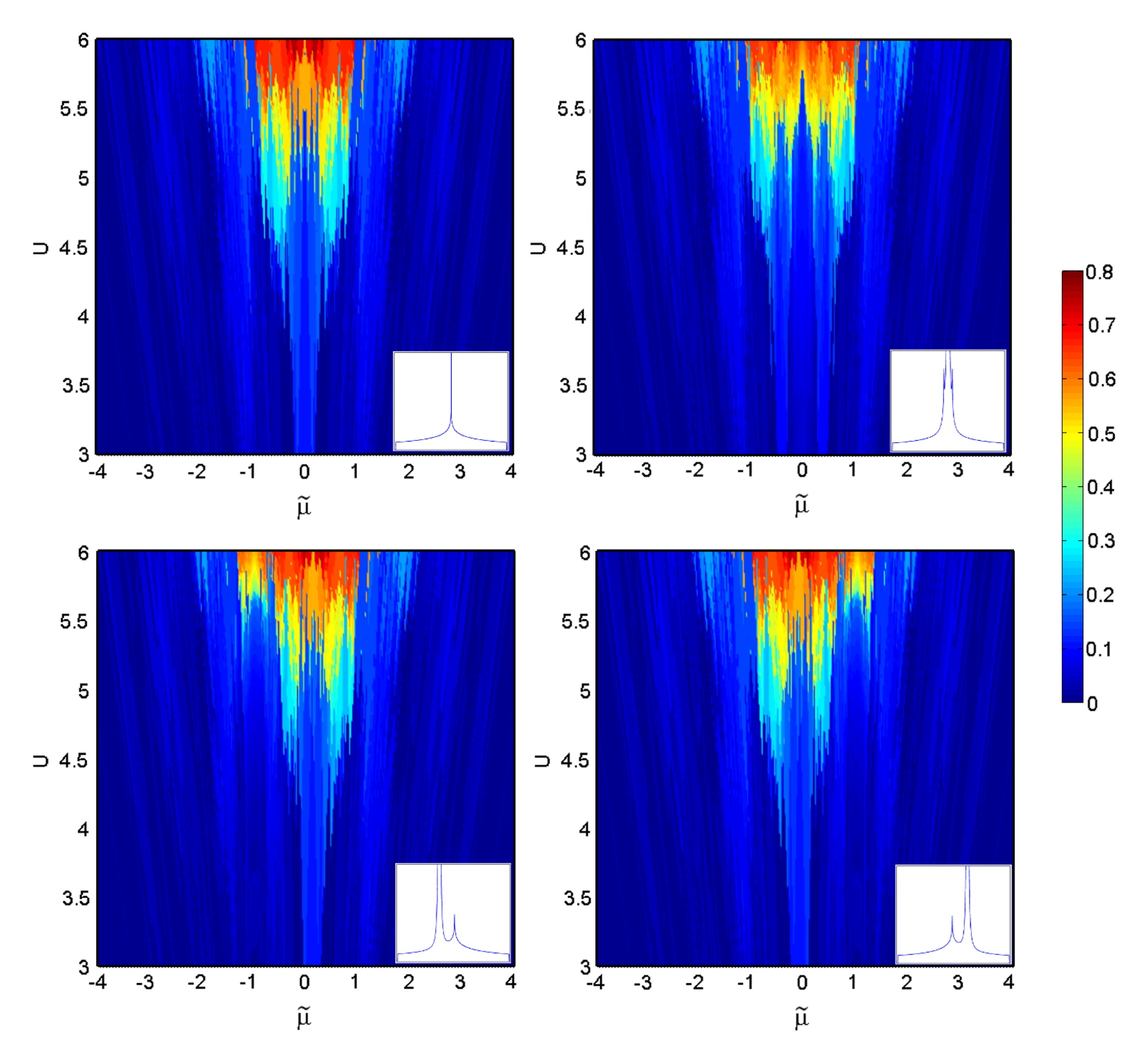
Figure 1: The variation of magnetization on the $U-\tilde{\mu}$ plane with (left to right, top and bottom column) no reservoir, reservoir at the peak of DOS, reservoir to the left and right of the band peak. The color code represents magnetization. Insets in each of the figures show the position of the reservoir (broadened for a nonzero $V$) with respect to the defect band. There is an enhancement of FM (red/yellow regions) when the Fermi level is close to the peak of the defect band (shown in insets).

The magnetization $M=\left<n_{\uparrow}\right>-\left<n_{\downarrow}\right>$ was calculated as the Fermi level is moved and for various fixed positions of the reservoir with respect to the defect band. The result, shown in Fig. 1, clearly shows the effect of adding a reservoir to the system - the magnetization is enhanced when the Fermi level is close to the reservoir. It shows how ferromagnetic regions in the phase space arise. The location of the FM region in the phase space strongly depends on the relative positions of the Fermi energy $\mu$ and $\varepsilon_{D}$. As $\mu$ passes through the reservoir, there is a strong mixing of the band and reservoir electrons. The Fermi level gets pinned at the resonant level and Stoner criterion is easily met. There is, of course, always a strong FM enhancement when the Fermi level is close to the peak of the defect band. In the absence of reservoir, the system exhibits a electron-hole symmetry at half-filling, as the band is symmetric about the peak. The defect band is expected to be spin-split when the Fermi level is close to the peak of the DOS (Stoner splitting), where the characteristics of this splitting is symmetric about the peak of the DOS due to the symmetry of the band. As discussed above, the effect of reservoir is most pronounced when the reservoir is placed off the peak of the DOS, thereby breaking the symmetry in the splitting. A higher splitting is seen when the Fermi level is close to the reservoir.

Note that this mechanism is independent of the nature of the underlying lattice. In fact, the special nesting in a square lattice generally favors AFM ground state at half-filling. But the mechanism discussed here can appear at any filling and the special topology of the Fermi surface is easily destroyed in a real system by beyond nearest-neighbor hopping.

The high magnetization obtained when the Fermi level is close to the reservoir is qualitatively similar to that obtained by Coey et al. from phenomenological calculations using a Lorentzian defect band [1] and a Lorentzian band for the reservoir [6].

3 Manganites

3.1 Introduction

Manganites came back to focus about seventeen years back owing to the discovery [7] of colossal magnetoresistance in these compounds. These are a class of manganese compounds of composition A_xB_1-xMnO₃ (A,B = La, Ca, Ba, Sr, Pb, Nd, Pr), which crystallize in the cubic structure of the perovskite mineral CaTiO₃ [8]. The basic unit of all the manganites is the MnO₆ octahedron with corner-shared oxygen and the central Mn^3+/4+ ion.

For manganites, the active electronic levels are the 5-fold degenerate d-levels of the Mn^3+/4+. In the octahedral environment of MnO₆ the $d^{5}$ is split into three-fold degenerate $t_{2g}$ lower level and two-fold degenerate $e_{g}$ upper level. The $t_{2g}$ levels are electronically inert and can be treated as localized spins with magnitude $S=3/2$. These localized spins are coupled to the itinerant $e_{g}$ electrons via Hund’s coupling. The itinerant electron system forms a band, the filling of which is controlled by the divalent cation doping.

The understanding of the magnetic effects in manganites is governed by the double exchange model by Zener [12], which gives a mechanism for hopping in the $e_{g}$ levels. The hopping is explained by the degeneracy of the Mn${}^{3+}\!\!-\!$O${}^{2-}\!\!-\!$Mn⁴⁺ and Mn${}^{4+}\!\!-\!$O${}^{2-}\!\!-\!$Mn³⁺ configurations. It involves a simultaneous transfer of an electron from Mn³⁺ to O^2- and from O^2- to Mn⁴⁺. But as the electrons in the itinerant band are coupled to the localized, $t_{2g}$ electrons via a Hund’s coupling, the localized electron at a site will favour an $e_{g}$ electron of parallel spin on the site.

It is well known that manganites have a large Hund’s exchange. In the limit this is infinite, each of the 5 d-orbitals will be spin split, the ‘wrong spin’ orbitals are never populated (as there are only 3 or 4 electrons in 3d orbitals of Mn ion). In this limit, the double occupancy at each orbital is also irrelevant. It suffices to work with three degenerate $t_{2g}$ orbitals and one $e_{g}$ orbital.

The nanostructured manganites show unusual magnetic behavior, different from the bulk. It has been observed in several manganites that the charge ordered, AFM manganites, when reduced to nanosize, develop ferromagnetic tendencies [9], presumably with the charge order also destabilized. Two possible scenarios have been put forward to ‘explain’ this: (i) the nanosize effectively increases the surface pressure, $P\sim S/R$, where $S$ is the surface tension and $R$ is the radius of the nanograin, assumed spherical. This excess pressure is supposed to destroy the charge order [10]. Pressure induced melting of charge and AF order has indeed been seen in bulk manganites. (ii) The enhancement of FM state comes from intrinsic causes [3, 4, 5]. The reconstruction at the surface of a nanograin reorganizes electronic states and favours double exchange. This would favour the FM tendencies over the superexchange between Mn ions and, at sufficiently small sizes, completely destabilize AFM order. The second view is emboldened by the observation [5] that the excess pressure on a typical nanograin is about 2-3 GPa, too low to melt the charge and AFM order. Besides, recent neutron scattering experiments [11] show no observable strain effects in bulk LaCaMnO₃ up to about 30 GPa pressure.

3.2 Model and calculation

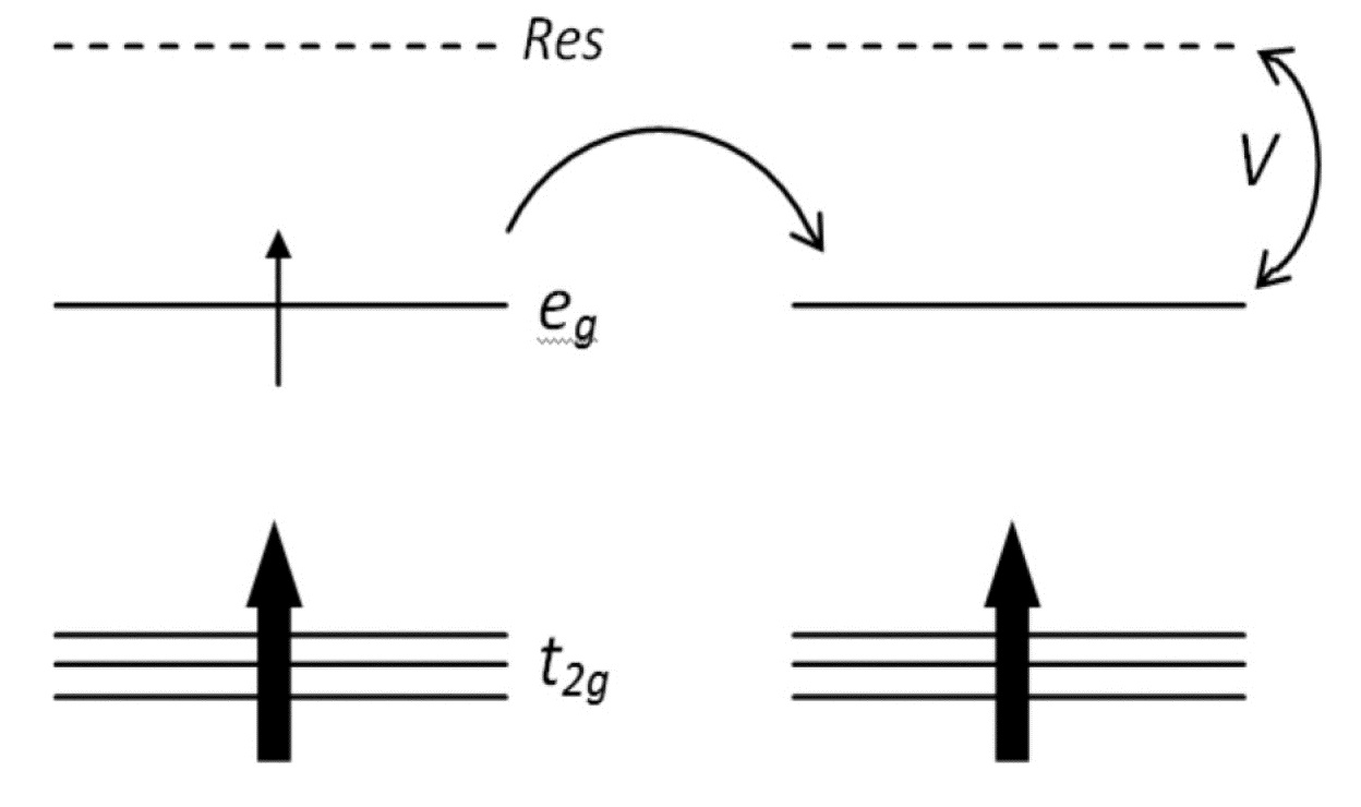
(a)

(b)

Figure 2: (a) The various levels at each site : The bottom $t_{2g}$ level with a localised classical spin, the middle itinerant $e_{g}$ level coupled to $t_{2g}$ level via Hund’s coupling and the top reservoir level coupled to the middle level. (b)The various states in Monte Carlo simulations, with the localised spin azimuthal angle $\theta_{i}$ colour-coded in $[0,\pi]$. The figures indicate, from left to right, a ferromagnetic, phase segregated and an antiferromagnetic state, obtained as $J$ is increased for a given $\mu$.

Following the discussions above, we use a single band (coming from the lone $e_{g}$ orbital) Hamiltonian coupled to a reservoir at each site. The basic manganite Hamiltonian is an itinerant $e_{g}$ electron system coupled to a localized $t_{2g}$ electrons via Hund’s coupling and a superexchange interaction between the localized electrons (leading to antiferromagnetism). The localized $t_{2g}$ electrons are treated as classical spins of magnitude $S=3/2$ pointing at an angle $\theta$ with the spin quantization axis (taken z-axis here). A schematic of this model is depicted in Fig. 2. The Hund’s coupling is taken as $J_{H}\rightarrow\infty$. In this limit, the hopping integral is modified by the projection of spin at site $i$ onto its nearest neighbour $j$ [13]. The overall Hamiltonian is

$$\mathcal{H}=\sum_{<i,j>}{\left(-t\cos{\left(\frac{\theta_{i}-\theta_{j}}{2}\right)}-\delta_{ij}\mu\right)c_{i}^{\dagger}c_{j}}+$$

$$V\sum_{i}{(c_{i}^{\dagger}d_{i}+d_{i}^{\dagger}c_{i})}+\varepsilon_{D}\sum_{i}{d_{i}^{\dagger}d_{i}}+$$

$$\tilde{J}\sum_{<i,j>}{\cos{(\theta_{i}-\theta_{j})}}$$ (3)

where $c_{i\sigma}/c_{i\sigma}^{\dagger}$ are the annihilation/creation operators for electrons in the band, $d_{i\sigma}/d_{i\sigma}^{\dagger}$ are the operators for the reservoir, $V$ is the coupling to the reservoir, $\varepsilon_{D}$ is the position of the reservoir with respect to the Fermi level and $\tilde{J}=\frac{9}{4}J$ is the superexchange parameter. In computation, all parameters are normalized by the hopping parameter $t$.

For this off-diagonal disordered Hamiltonian we use a hybrid Monte Carlo simulation [3] where the Fermionic part was solved by exact diagonalization and the annealing over classical variables were performed by Metropolis algorithm. The simulations were carried out on a $12\times 12$ square grid with periodic boundary condition. A vector $\Theta=[\theta_{1},\theta_{2},\dots\theta_{N}]$ uniformly distributed in $[0,\pi]$ is chosen to start with, where $\theta_{i}$ is the azimuthal angle of the localized classical spin at site $i$. At each step, two $\theta_{i}$’s were modified by a random amount in $\left[-\frac{\pi}{16},\frac{\pi}{16}\right]$ and the Hamiltonian was diagonalized for this new $\Theta$ vector. The choice between the new and the old states was done using the Metropolis-Hastings algorithm. The system was annealed in this fashion from $\beta=1$ to $\beta=25$ in 100,000 iterations. The spin-spin correlation and free energy was averaged out over a further 50,000 iterations.

3.3 Results

We obtain the results for both with and without the reservoir. In order to obtain the phase diagram, simulations were carried out for various parameter values. Typical magnetic configurations that appear in the ground states of the MC simulation are shown in Fig. 2(b). Ferromagnetic, phase segregated and antiferromagnetic states are shown. It is not always possible to delineate different phases (particularly close to a phase transition). In the theormodynamic limit, there will be a small splitting between the spin up and spin down bands. However, for the small number of sites we work in ($12\times 12=144$), a better quantitative method is to find the nearest neighbor spin spin correlations, which is -1 and +1 for saturated AFM and FM, respectively. The phase boundary is given by $\left<S_{i}S_{j}\right>=0$. The resulting phase diagram is plotted in Fig. 3(a) and Fig. 3(b). The value of $\mu$ is varied from $-4$ to $0$, corresponding to zero to half filling, i.e., the value of $x$ varying from $0$ to $1$ in, say, La_1-xCa_xMnO₃.

Clearly the presence of a huge number of states leads to a situation where there could well be degenerate (or nearly degenerate) solutions for the ground state. The competing interactions of superexchange and double exchange favouring the AFM and FM correlations respectively, lead to first order transitions and consequent phase segregation [3]. Indeed, similar situation obtains here too. As observed in the simulations, the phase transition occurs via a phase segregated state. It is worthwhile to mention the possibility of a canted spin state  [14]. From a mean field calculation, it was shown that the AFM-FM transition in the double exchange Hamiltonian should proceed through two continuous transitions via a spin canted state. However, the canted state has never been found to be the ground state in any simulation [3]. The transition is first order with a phase-segregated (two-phase coexistence) region as we also confirm.

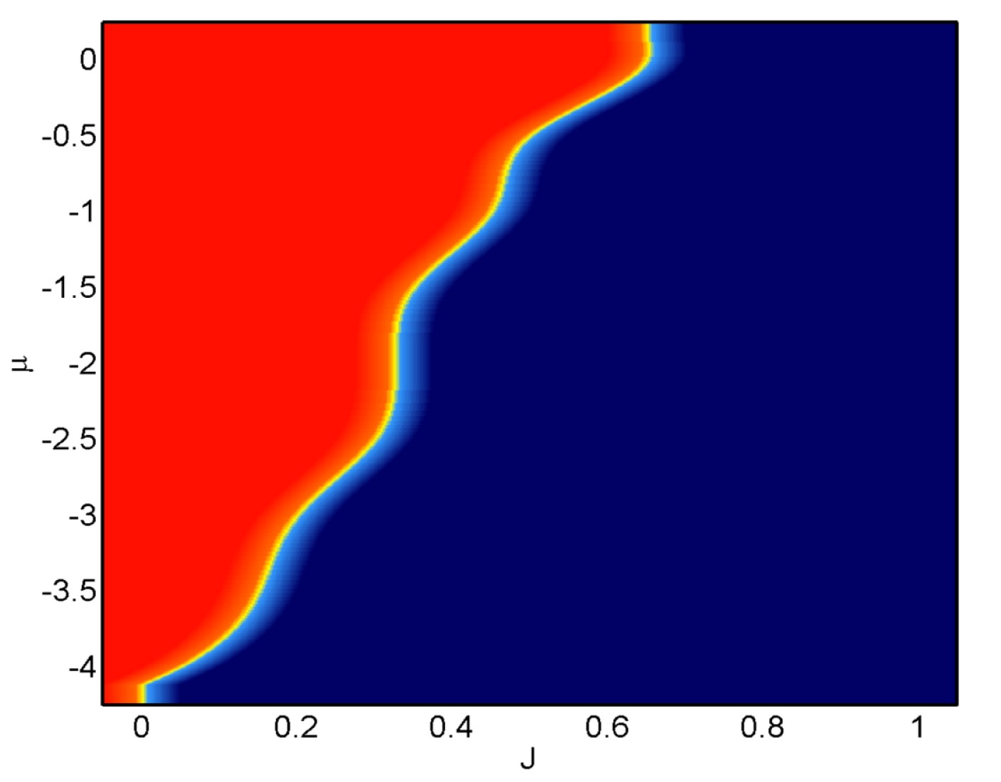
(a)

(b)

Figure 3: Phase diagram of the manganite system in absence of reservoir on (a)$J-\mu$ and (b)$J-N$ planes. The colour codes are same as in previous figure.

The addition of reservoir introduces two new parameters, the coupling $V$ and the position of the reservoir, $\varepsilon_{D}$ with respect to the Fermi level. In all the calculations, the Fermi level and the position of the reservoir are held constant, and the coupling is turned on from $V=0$ to $V=0.3$. The spin-spin correlation is computed, for the two cases of zero coupling (which is equivalent to no reservoir) and with a finite coupling. These calculations were repeated for various positions of reservoir with respect to the Fermi level. The variation in spin-spin correlation is calculated for $\mu=0$ (filling = $0.5$) and $\mu=-1$ (filling = $0.2$), as plotted in Fig. 4(a) and 4(b), respectively.

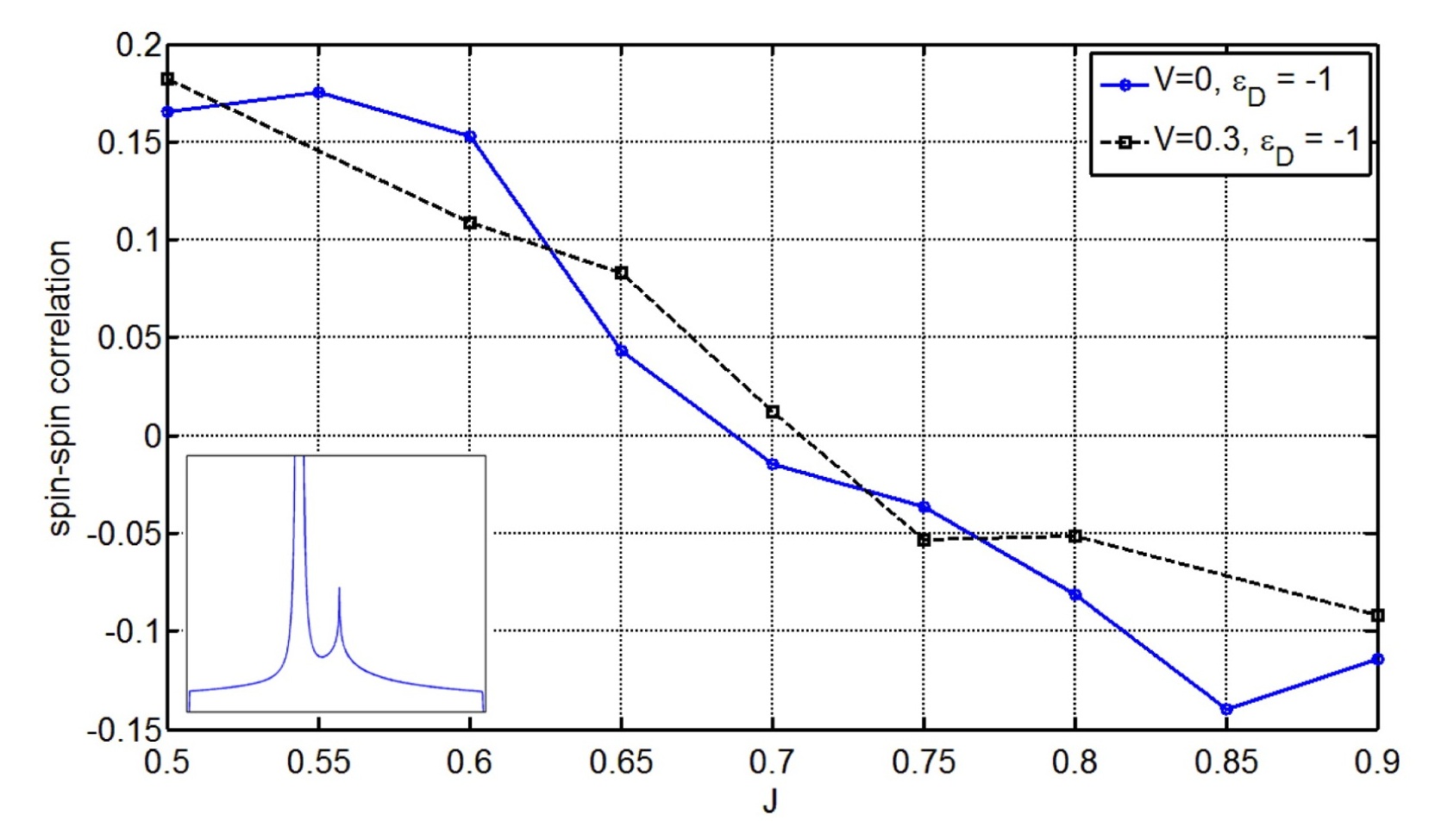
(a)

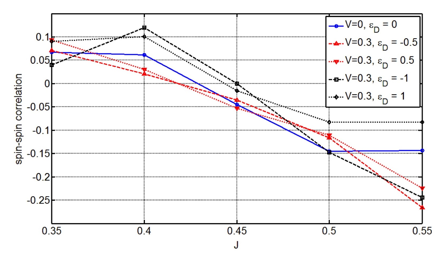
(b)

Figure 4: Variation in the spin-spin correlation due to reservoir at (a)$\mu=0$ and (b)$\mu=-1$

On addition of the reservoir (with $\varepsilon_{D}=-1.0,\,V=0.3$) to the system below the Fermi level at half-filling, the filling of the band decreased from 0.5 to 0.47; electrons have been drained to the reservoir. At half filling, each site has one electron and delocalization is not possible. However, when holes are introduced in this system, the holes will delocalize all over the lattice, leading to significant kinetic energy gain (enhanced double exchange) and ferromagnetism is enhanced in the ground state. As seen in Fig. 4(a), a comparison between the dashed ($V=0.3$) and contunous lines ($V=0$) indicate enhanced FM correlation in the former, indeed higher spin spin correlation imply more ferromagnetic tendency. The corresponding location and broadening of the reservoir is also shown in the inset. The presence of the reservoir moves the peak of the band towards higher energy by $V^{2}/t$, thereby leading to decrease of the filling of band for $\mu=0$. Hence, the reservoir induces ferromagnetism by introducing holes in the band. For the second case of $\mu=-1,\,\varepsilon_{D}=\pm 1$ (Fig. 4(b)), the reservoir acts as a donor and drives the system towards ferromagnetism again. Here, as the original band-filling is low ($0.2$ in this case), the delocalization energy can be increased only by addition of electrons. The reservoir now acts as a donor and accomplishes the same objective as above.

4 Conclusions

It is shown that the charge transfer ferromagnetism model introduced by Coey et al. is able to predict the hugely enhanced ferromagetic order seen in the transition metal doped oxide nanoparticles qualtitatively. More importantly, the observed enhancement of FM tendencies in nanoparticles of manganites also finds a resolution within the same framework. Surface magnetic probes like $\mu$SR may be a possible tool that can establish the proposed scenario in manganites.

References

- [1] J. M. D. Coey, P. Stamenov, R. D. Gunning, M. Venkatesan and K. Paul, New J. Phys. 12 (2010) 053025.
- [2] J. M. D. Coey, Kwanruthai Wongsaprom, J. Alaria and M. Venkatesan, J. Phys. D: Appl. Phys. 41 (2008) 134012.
- [3] E. Dagotto, T. Hotta and A. Moreo, Phys. Rep. 344 (2001) 1.
- [4] H. Zenia, G. A. Gehring, G. Banach, and W. M. Temmerman, Phys. Rev. B 71 (2005) 024416.
- [5] S. Kundu, T. K. Nath, A. K. Nigam, T. Maitra and A. Taraphder, arXiv:1006.2943 (2010): Jour. Nanoscience and Nanotech. (2011) to be published.
- [6] Vatsal Dwivedi, P. Stamenov, C. Porter and J. M. D. Coey, Unpublished results.
- [7] S. Jin, T. H. Tiefel, M. McCormack, R. A. Fastnacht, R. Ramesh and L. H. Chen, Science 264 (1994) 413.
- [8] Colossal Magnetoresistive Oxides edited by Y.Tokura, Gordon and Breach Science, Singapore, 2000.
- [9] S. S. Rao, K. N. Anuradha, S. Sarangi, and S. V. Bhat, Appl. Phys. Lett. 87, 182503 (2005).
- [10] Tapati Sarkar, A. K. Raychaudhuri, and Tapan Chatterji, Appl. Phys. Lett. 92, 123104 (2008).
- [11] Z. Jirák, E. Hadová, O. Kaman, K. Knížek, M. Maryško, E. Pollert, M. Dlouhá and S. Vratislav, Phys. Rev. B 81 (2010) 024403.
- [12] C. Zener and R. R. Heikes, Rev. Mod. Phys. 25 (1953) 191.
- [13] P. W. Anderson and H. Hasegawa, Phys. Rev. 100 (1955) 675.
- [14] P. G. de Gennes, Phys. Rev. 118 (1960) 141.