Emergence of Homogeneous and Isotropic Loop Quantum Cosmology from Loop Quantum Gravity: Lowest Order in
Chun-Yen Lin
Physics Department, University of California
Davis, CA 95616
Abstract
To derive loop quantum cosmology from loop quantum gravity, I apply the model given in [48] to a system with coupled gravitational and matter fields. The matter sector consists of a scalar field serving as a cosmological clock, and other fields providing physical spatial coordinates and frames. The physical Hilbert space of the model is constructed from the kinematical Hilbert space of loop quantum gravity, and the local observables in the physical Hilbert space are constructed using the matter coordinates and frames. A specific coherent physical state is then chosen, whose expectation values of the local observables give rise to homogeneous, isotropic and spatially flat gravitational and fields at a late clock time. The equations governing these fields may be derived using the symmetry of the physical Hilbert space. When the matter back reactions from are negligible, the result gives a specific loop quantum cosmological model in the approximation, with calculable higher order corrections.
1 Introduction
Loop quantum cosmology refers to a set of quantum cosmological models [24, 26, 27, 28, 29] incorporating key features of loop quantum gravity [35, 36, 37]. As a candidate fundamental theory of gravity, loop quantum gravity has a rigorously defined kinematical Hilbert space describing quantum spatial geometry that is discretized in Planck scale. Building on this kinematical foundation, theorists are now tackling the challenge of obtaining the dynamics. By introducing the key features of loop quantum gravity into symmetric cosmological models, loop quantum cosmology aims to explore the effects of the quantum geometry in cosmic evolution.
Loop quantum cosmology bypasses much of the complexity in loop quantum gravity because of symmetry reductions, and its dynamics is well-defined and extensively studied. However, the simplifications come with ambiguities: in the same physical setting, different symmetry reduction procedures can lead to distinct loop quantum cosmological models. Thus, several models in loop quantum cosmology have been proposed based on different physical considerations. However, for an isotropic, homogeneous and universe with massless scalar matter fields, several robust features prevail in the family of models [24, 26, 27, 28, 29]: 1) they reproduce classical FRW cosmology in their large-scale semi-classical limits; 2) the semi-classical limits deviate from FRW cosmology near the initial singularity, replacing it with a well-behaved bounce of the scale factor [33, 34]; 3) with a proper coherent state, an in-built slow-roll inflation phase occurs following the bounce [31, 32]. These results are obtained through both numerical and analytical approaches to different degrees of approximation. Moreover, the study of the cases with either negative , inhomogeneity or anisotropy [24, 45, 21, 22, 23] also finds a bounce in Bianchi I, II and IX anisotropic models.
With its rich implications, it is essential for loop quantum cosmology to find its root in loop quantum gravity, so that the implications can be attributed to fundamental principles. On the other hand, people are searching for observable predictions in loop quantum gravity, hoping to derive loop quantum cosmology.
Aiming at these goals, I apply the model proposed in [48] to a cosmological system with . The matter sector of the system consists of a chargeless and massless scalar field and other matter fields denoted as . These matter fields live in the quantum geometry of space given by the gravitational sector of the system. The model describes this system using the kinematical Hilbert space of loop quantum gravity, called knot space.
Based on knot space, the physical Hilbert space of the model is built under concrete assumptions. Local observables in for gravitational and fields are constructed, using spacetime coordinates provided by the matter fields [38, 39]. Specifically, the field serves as the cosmological clock, and the fields in provide the spatial coordinates and frames. For a suitable coherent state in , the expectation values of these observables give rise to emergent classical gravitational and fields in the spacetime manifold. In our context, we will choose a coherent state that gives homogeneous, isotropic and spatially flat emergent fields at an early clock time. The cosmic evolution of the emergent fields will be calculated using the symmetry of . When the matter back reactions from sector are negligible, the result conforms with a specific loop quantum cosmological model at order . To the approximation, it recovers FRW cosmology in large scales and resolves initial singularity by the big bounce.
2 Kinematic Hilbert Space of Loop Quantum Gravity
This section is a brief introduction to the kinematics of loop quantum gravity including gravitational and matter sectors. The kinematical Hilbert space, called knot space, gives a background independent description of the spatial quantum geometry and the resident matter fields.
2.1 Ashtekar Variables for Gravitational and Matter Fields
Loop quantum gravity is based on a canonical general relativity in the Ashtekar formalism [15, 16, 17]. This formalism describes gravitational fields in a form similar to that of matter gauge fields.
Traditionally, canonical general relativity uses spatial metric and extrinsic curvature defined in the spatial manifold as phase space variables [15, 16, 17]. As an alternative, triad fields consisting of three orthonormal vector fields can be used in place of the spatial metric. In the basis of and its inverse , the spatial Levi-Civita connection and extrinsic curvature take the forms and . Ashtekar variables are related to through a canonical transformation by [16][17]:
| (2.1) |
where the real number is called the Immirzi parameter. By construction, the fields are densitized triad fields, and the fields are gauge fields. The variables have the non-vanishing Poisson brackets:
| (2.2) |
where is Newton’s constant. Note that one may replace the symmetry group with in this formalism, since and share the same Lie algebra.
Matter fields with a gauge group can be included in this formalism [18, 19, 20]. Using the triad basis, we describe the fermion, scalar and gauge fields by , and . Here , and i are respectively (gravitational spin ) , and adjoint indices.
In this formalism, the action of general relativity possesses the following local symmetries: 1) time re-foliation invariance, which introduces the Hamiltonian constraint ; 2) spatial diffeomorphism invariance, which introduces the momentum constraint ; 3) local invariance, which introduces the Gauss constraint ; 4) local , invariance which introduces the Gauss constraint . Each constraint is a functional of the dynamical fields and the Lagrangian multipliers , , , (the bars indicate their non-dynamical nature). The first three constraints result from spacetime diffeomorphism symmetry, and they consist of pure gravitational and matter terms:
| (2.3) |
Here, we give the explicit forms of the pure gravitational terms, denoting :
| (2.4) |
The explicit forms of the matter terms depend on the matter fields, which we would specify later.
The three constraints form a closed algebra with structure functionals independent of the explicit forms of the matter terms. Denoting to be the commutator, and setting , the algebra is given by
| (2.5) |
where denotes a Lie derivative and
| (2.6) |
2.2 Knot Space
In QCD, the generalized electric flux and magnetic holonomy variables are powerful in capturing non-perturbative degrees of freedom of gluon fields. The Ashtekar formalism enables an analogous treatment of gravitational fields. Gravitational holonomy and flux variables are signatures of loop quantum gravity [36, 35, 37], and they capture non-perturbative degrees of freedom of gravitational fields. The holonomy variable over an oriented path (the bar indicates that is embedded in the spatial manifold ) gives the parallel transport along the path by the connection fields . The flux variable over an oriented surface gives the flux of through the surface. Explicitly, we have:
| (2.7) |
where denotes path ordering along , and the -valued gravitational holonomy is written in the spin matrix representation. The matter variables compatible with the gravitational flux and holonomy variables are the following [18, 19, 20]. The gauge fields are described by the holonomies in representations , and the fields are described by the flux variables . If is a generic point in , the fields are described by the irreducible tensors obtained from their Grassmann monomials of degree , and the spinor momenta are described by . The fields are described by called point holonomies in representations , and the momenta are described by . This new set of gravitational and matter variables are collectively called loop variables. The kinematical states of loop quantum gravity [36][35][37] are called knot states, and they are functionals of the configuration Ashtekar variables via the corresponding loop variables .
A knot state is given by an invariant product of loop variables defined on a graph in , so it solves the Gauss constraints. Further, the knot state is only sensitive to the embedding of the graph up to a spatial diffeomorphism , so it also solves the momentum constraint. Define an embedded graph in to consist of smooth oriented paths , called edges, meeting at most at their end points , called nodes (the bars again indicate that is embedded in ). Carrying loop variables, an embedded colored graph is defined by: 1) an embedded graph ; 2) an spin representation and a group representation assigned to each edge; 3) generalized and Clebsch-Gordan coefficients (intertwiners) and , a point holonomy representation and a Grassmann monomial degree assigned to each node. The assignment of , , , , and gives a scalar functional :
| (2.8) |
where denotes the invariant contraction. An element drags to and transforms to . Note that for every , there is a subgroup of that leaves the graph invariant, maintaining the set of all the edges and their orientations. There is also a subgroup of that acts trivially on . Thus we have the graph symmetry group . The group averaging operator serves to erase the embedding information from , and it is defined as:
| (2.9) |
where is the number of elements in , and is a colored graph obtained from the embedded colored graph by erasing its exact embedding.111 Note that when , we have . The result is a knot state. Such a state is determined by a colored graph , and is invariant since . The inner products between knot states are given by (generalized) Ashtekar-Lewandowski measure [36][35][37][20], with which the set of all knot states gives an orthonormal basis:
| (2.10) |
This basis spans knot space , the and invariant kinematical Hilbert space of loop quantum gravity.
Canonical quantization of loop variables leads to the operators of the form , where may be , , or . However, does not preserve since is not invariant. To respect symmetry, we now replace by a dynamical object that assigns to each , such that transforms together with under transformations. Setting to contain exactly one representative from every , one can construct by specifying for every . More formally, each dynamical object is a map satisfying for any and some . Then, we can define invariant operator as:
| (2.11) |
For example, one can construct invariant flux and holonomy operators using a dynamical surface and a dynamical path :
| (2.12) |
The two operators are respectively differential and multiplicative operators acting on , and their invariant products give gravitational operators in . Since determines the spatial metric, the spatial area and volume operators are made up of the flux operators [36, 35, 37]. as a differential operator acts on the gravitational sector of in a way that satisfies the Leibniz rule. Specifically, when intersects with only at its node , we have:
| (2.13) |
where is or when is above or below in an infinitesimal neighborhood of , and is if otherwise; is or when is the source or target of .
The area operator in loop quantum gravity is derived from regularizing the classical expression in terms of the flux variables. The resulting area operator of a dynamical surface is [8]
| (2.14) |
Remarkably, knot states are eigenstates of for any dynamical surface . Set to be a point where intersects transversely with , and let represent the spin carried by the edge containing the point . One can then easily check that
| (2.15) |
where the Planck length is defined by . It is clear that the spectrum of area operators in is discretized, built from multiples of small quanta of order of .
The volume operator in loop quantum gravity also results from the regularization of the classical expression using the flux variables, but with much more complicated technicalities. Also, there are a variety of different regularization approaches that lead to different operator forms [9, 10]. Here we will follow the one introduced in [10]. The volume operator given by this approach acts on with a set of flux operators over dynamical surfaces intersecting only at the nodes. With the help of , the action of the volume operator for a dynamical region boils down to [10]:
| (2.16) |
By the volume operator for a region acts only on the nodes of a knot state contained in . Further, each node-wise operation on the spin network state is given by the sum of the triplets of the action on the edges meeting at the node. Therefore, the volume operator changes only the intertwiners of the nodes of . Consequently, there is a volume and area eigenbasis for knot space, consisting of states given by a definite and .
Each member of the eigenbasis for the area and volume operators has the following interpretation: a certain quantum of volume is assigned to each node of the state, and a certain quantum of area is assigned to each edge of the state. Through this basis, provides a concrete description of quantum spatial geometry – the networks carrying Planck sized units of areas and volumes, associated with their edges and nodes.
The remaining constraint to be imposed for a physical Hilbert space is the Hamiltonian constraint. Adhering to the polymer-like structure of knot states, the standard Hamiltonian constraint operator [36, 37, 20] is quantized from a regularized discrete expression approximating . In the discrete expression, the curvature factors in are approximated by holonomies along a certain set of tiny loops. The quantization then leads to that contains holonomy operators based on these loops. Therefore, the action of on a knot state involves a change in the graph topology that adds the set of tiny loops to . Moreover, since a non-constant Lagrangian constraint is not invariant, does not preserve in general. With constant the action of preserves , but it is intricate and changes the topology of the graphs. As a result, constructing a physical Hilbert space annihilated by is a major challenge, which is currently tackled by both canonical approaches [35, 37, 40, 12] and the path integral formalisms [37, 42, 43].
3 The Model
In our model, we will modify into a graph topology preserving operator defined on . The greatly simplified setting will allow us to apply the group averaging method to construct the physical Hilbert space of the model, based on certain concrete assumptions. A set of local Dirac observables in will be obtained using the clock constructed from the field and spatial matter coordinates and frames from the sector.
3.1 Modified Hamiltonian Constraint Operator and Physical Hilbert Space
For each embedded graph , we label each of its nodes with an integer and each of its edges connected to the node by an integer pair (the range of depends on in general).222Note that each edge has two labels since it contains two nodes. For a given , we denote its node by , and the oriented path starting from and overlapping exactly with its edge by (fig.1a). To each pair we assign a minimal oriented closed path that lies in , containing the outgoing path and incoming path (fig.1a). Using these labels, we define a set of dynamical nodes , satisfying such that is one-to-one. Corresponding to a given , we define a set of dynamical paths satisfying and such that is one-to-one. The dynamical closed path is then determined by the outgoing and incoming dynamical paths. We also define a set of dynamical spatial points , where ranges from to infinity, such that holds for exactly one for every and .333The spatial manifold contains uncountably many spatial points, but we use only countably infinite set in correspondence to the discrete structure of . Also, the one-to-one correspondence between and is obvious had we taken for any to be the set of in . Here we define to be a countably infinite subset of , while maintaining this natural condition. Notice that there are infinitely many distinct sets of dynamical nodes, paths and spatial points satisfying the above. This ambiguity comes from the arbitrariness of identifying the nodes and edges between different knot states, due to the absence of a reference background in .

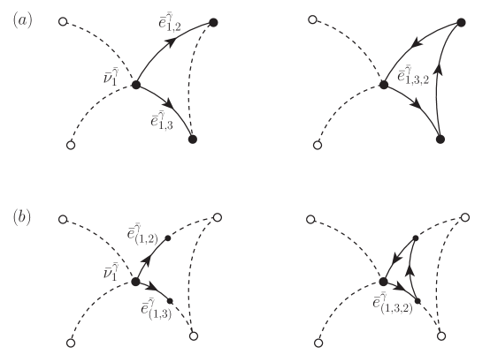
The modification from into – a crucial step for the model– contains two elements [48]. First, is replaced by a invariant lapse function , which is a function of a set of dynamical spatial points . Recall that the embedded spatial point transforms under just as does. That means the classical counterpart of is the field that transforms as a scalar field. Therefore, in proper semi-classical limits, the operator is expected to approximate the invariant instead of . Second, the tiny loops (fig.1b) that define the holonomy operators in are replaced by the new set of closed paths (fig.1a) that are contained in the graphs of knot states. By using the corresponding new set of holonomy operators, preserves the graph-topology of knot states. Since preserves both symmetry and the graph topology, it is an operator in any subspace with one specific graph topology . For simplicity, the model’s kinematical Hilbert space is set to be with the graph topology of a lattice torus , which has nodes and six edges connected to each of the nodes. Restricted to , we have and for and , and will be a square closed path overlapping with exactly four edges in
The modification applied to the gravitational term of results to the new gravitational term , which acts on as (set ):
| (3.1) |
where we have
| (3.2) |
Here, the total volume operator is defined as
| (3.3) |
The modification applied to the matter term in [20] results to the new matter term , whose explicit form depends on the matter content. Similar to the pure gravitational term, it is also constructed from the loop operators in , and acts on as:
| (3.4) |
where denotes the end node of .
Finally, the Hamiltonian constraint operator for our model is given by the self-adjoint sum of the gravitational and matter terms:
In order to compare the model with loop quantum cosmology, we will choose an identical physical setting. In this setting, gravitational fields are fully coupled to the chargeless, massless real scalar field , while all other matter fields with small back-reaction are collectively named as . The classical constraints in this case are:
| (3.5) |
Note that the functionals , and are the constraints for the subsystem of only gravitational and fields, and themselves satisfy the algebra .
The loop operators for field are the point holonomy opreators with arbitrary real , and the conjugate momenta operators . Their non-vanishing commutators are given by
| (3.6) |
Corresponding to , we have . The modified operator formed by quantizing is given by [20]:
| (3.7) |
where
| (3.8) |
with a small real number whose exact value is unimportant in our context. The modified Hamiltonian constraint operator in our setting is then given by:
| (3.9) |
Recall that our kinematical Hilbert space is already and invariant. To obtain the physical Hilbert space of the model, we still need to impose the remaining symmetry generated by with arbitrary based on arbitrary . These unitary operators form a faithful representation of a group , that is
| (3.10) |
where is an arbitrary lapse function based on an arbitrary , and means that we identify two expressions if they give the same operator in . The physical Hilbert space of the model is constructed using group averaging procedure under the assumptions: (1) the existence of the left and right invariant measure for ; (2) the operator defined by
| (3.11) |
maps into . The two conditions hold in minisuperspace models [11, 1, 2], but remain to be proven for the model. Under these assumptions, the inner product between any two states and may be defined as
| (3.12) |
The physical Hilbert space of the model is the space spanned by . By construction, is invariant under the action of with arbitrary , and satisfies the modified Hamiltonian constraint. Each element in is a solution to the quantized Einstein equations, and therefore is a quantum state of spacetime with the matter fields.
3.2 Local Dirac Observables
The model obtains its local Dirac observables using clocks, spatial coordinates and frames given by the matter fields. For an arbitrary set of dynamical nodes , one may construct a set of self-adjoint, commuting matter operators consisting of scalar operators diagonalized by the knot state basis of , current operators and conjugate current operators ( for the vector currents; for the spinor currents). The operator triplet will serve as spatial coordinate operators, and will be spatial frame operators, and will be the clock operator. In our setting, the cosmological clock field is chosen to be:
| (3.13) |
provided by the field.
Classical gravitational fields in the Ashtekar formalism are tensors. In the model, the invariant components of the fields are described relative to the matter spatial frames. Explicitly, for any we define
| (3.14) |
In canonical general relativity with the matter spatial coordinate field , we can obtain a invariant and spatially local variable by integrating over . Analogously, the model uses a normalized Gaussian distribution with finite width and defines:
| (3.15) |
for any , where the coordinate volume element operators are given by:
It is crucial that the spatially local operators obtained in do not depend on the choices of the dummy variables and . The invariant operators are localized by referring to the spatial matter coordinates.
To specify time using the clock field , we construct an operator that maps a spacetime state to the spatial slice state on which . With denoting an operator acting on , the operator is defined by:
| (3.16) |
where the symmetrization in the ordering of is applied. The resulting local Dirac observables in are given by
| (3.17) |
In the following, in will serve as an index running over the matter coordinates and frames contracted with the non-zero test functions . The variables thus contain information about the momenta of the reference matter fields.
Finally, applying , and to the fields of concern we obtain the relevant localized observables. In the following, we will give the dynamics of , , , , in a certain “physical gauge” of matter coordinates and frames that is fixed by .
3.3 Conditions on Matter Coordinates and Frames
Our next step is to choose a proper physical state to derive semi-classical limits from the model. In order to give sensible descriptions, the localized observables must refer to well-behaved matter coordinates and frames. So there are conditions to be imposed on the matter sector of , which provides the matter coordinates and frames.
For the clock, we require any two spatial slices of with and to be related by causal dynamics, so that either one of them can be used to reconstruct the spacetime. In the model, this condition is imposed as:
| (3.18) |
When is satisfied, we have:
| (3.19) |
More generally, denoting by a function of linear operators in a Hilbert space, we have
| (3.20) |
On each spatial slice , we will also impose spatial coordinate conditions to properly describe gravitational and fields. Denote an arbitrary function of the gravitational and field operators based on and as:
We require that there exist and such that:
| (3.21) |
with a certain set of values and satisfying . Here, represents the physical nodes at clock time for an observer using the spatial matter coordinates . Naturally, there is also a set of physical spatial points agreeing with , such that for . Condition says that each physical node acquires a matter spatial coordinate value, and that the matter frames are physically orthonormal to each other at each physical node. The spatial coordinate condition can now be imposed on the map . Analogous to the coordinate maps on a torus manifold, the map should appear smooth in large scales at most of the physical nodes except at some where coordinate singularities occur. We demand for , where is small enough that the map appears continuous at large scales. Also, for any the set should define a parallelepiped in up to an error of so the map appears smooth at large scales. Notice that once is satisfied, the coordinate conditions can be achieved easily through a redefinition of coordinates .
Using a lapse function satisfying with an arbitrary function , we can apply to :
| (3.22) |
Copying the form of shown in , is given by:
| (3.23) |
where is
| (3.24) |
and
| (3.25) |
Copying the form of shown in , is given by:
| (3.26) |
where
| (3.27) |
Further, the well-behaved matter coordinates and frames also lead to simple algebraic relations between the spatially local operators acting on . From now on we set a variable to take values in . Also, define as the operator localized from which is diagonalized by the basis . The state has eigenvalue if the embedded edge of overlapping with has the same orientation as and has eigenvalue if otherwise. The algebraic relations between the spatially local operators are the following:
| (3.28) |
This conditional algebra enables further calculations after the approximations are made.
Lastly, we also require to give the momenta of the matter coordinates and frames:
| (3.29) |
The matter coordinates and frames specify a gauge for the gravitational sector. Locally at the moment , this gauge is characterized by and . For this paper, we require the simple gauge condition:444Note that the vaules of can be adjusted by clock-time dependent redefinitions of the matter coordinates and frames
| (3.30) |
which gives a comoving frame in the cosmological setting that will follow later.
3.4 Coherent States and Emergent Fields
We have required the state to satisfy the quantum coordinate conditions and , such that the set of local observables and would give meaningful descriptions around the moment . Since our goal is to obtain semi-classical limits, we impose coherence conditions on the gravitational and field sector of as:
| (3.31) |
Since the clock is built from field, the conditions imply:
| (3.32) |
which specifies the value in . Additionally, we also want the expectation values to appear continuous in terms of the spatial coordinates for a semi-classical state. Therefore, for any two and that share a common node and form a smooth path, we will impose (recall that for ):
| (3.33) |
Because of the algebraic relation , we expect the gravitational and field sector’s solutions to and to exist. These conditions say that has sharply defined, approximately continuous values for the local observables at clock time . Therefore, is expected to be semi-classical around that moment.
To make contact with classical general relativity, the model maps the expectation values in to the classical field values, using the matter coordinates as a common reference. For an explicit example, we will first pick a simple spatial matter coordinate system. Recall that the lattice torus can be constructed by identifying the opposite boundary faces of a lattice rectangular prism , which consists of the vertices and links (the bars indicate the embedding in ). Such construction naturally gives a coordinate map . Also, the approximated spatial coordinate space is naturally a rectangle region inside of .
Once matter spatial coordinates are chosen, our model identifies every disjoint from with an embedded path in , under the guidance of the matter coordinate values. In our case, is identified with the oriented path that goes from the vertex to the vertex , which overlaps exactly with the link connecting the two vertices. Subsequently, we choose a cell decomposition dual to , dividing into a set of cells that are parallelepipeds up to errors of . Each cell uniquely contains a vertex , and the boundaries of consist of a set of faces whose each element intersects transversely with a unique link . Suppose links and , we denote the oriented surface overlapping with and having the same orientation as . Then, model uses a fitting algorithm that maps the expectation values and to the values of the smooth fields and defined in . The fitting algorithm is required to obey the following rules:555 Note that such an algorithm is guaranteed to exist, since we are fitting the smooth fields with infinite degrees of freedom to the finitely many data points given by the expectation values of the local observables.
| (3.34) |
In the rest of the paper, we will use the spatial coordinates with for , which makes a right cubical cell, and a square oriented surface. The choice of , the cell decomposition , and the fitting algorithm described above are restricted but non-unique. However, any choice satisfying the restrictions gives a valid correspondence between and the emergent fields.
4 Physics in Homogeneous, Isotropic and Spatially Flat Sector
The paper [48] has shown that the fields and determined by reproduce vacuum general relativity up to quantum gravitational corrections, when matter back reactions can be ignored. In the following a similar calculation will be done, assuming gives homogeneous, isotropic and spatially flat emergent fields and at a late initial time . In comparison with [48] the calculation will be done with two extensions: 1) while the matter back reactions from will still be ignored, the full interaction between gravitational and fields will be considered; 2) the quantum gravitational corrections will be evaluated to . The calculation will give the effective equations governing the fields and , which will be compared with the effective equations in different models of loop quantum cosmology.
4.1 Emergent Constraints and Diffeomorphism Algebra
For notational simplicity, we will denote the collections of the spatially local gravitational, field and operators as . One can evaluate the n-fold commutator by first applying :
| (4.1) |
where is given by carrying out all commutators. Then we use , and to obtain:
| (4.2) |
Recall that is the Hamiltonian constraint for the subsystem of only gravitational and fields. The sector serves as a background for this subsystem. Since the spatial coordinates are given by the sector, the lapse functions are Lagrangian multipliers for the subsystem. According to , the Poisson brackets, to all orders in , with arbitrary reproduce the full (off-shell) diffeomorphism algebra between , and in the semi-classical limit of , up to corrections of .
Moreover, the symmetry implies that:
| (4.3) |
Separating the contributions involving or and denoting them as , we have:
| (4.4) |
where we replace with using the spatial coordinate condition . The term represents the matter back reaction from the sector, and we will use to denote generic matter back reactions from the sector in the following. According to , the emergent gravitational and fields satisfy:
| (4.5) |
Therefore, the emergent gravitational and fields as a subsystem are on-shell up to corrections .
4.2 Homogeneous, Isotropic and Spatially Flat Dynamics
The coherent state gives the dynamics of , through the corresponding at various . We now evaluate this clock time dynamics in a symmetrical setting.
Before the calculation, we need to set up a homogeneous, isotropic, and spatially flat initial condition at some late clock time . Since the field serves as the clock, it is clear that , and implies that is spatially constant. We require the coherent state to give homogeneous , and , such that:
| (4.6) |
where identifies with . Note that satisfy as required, and it also implies that
| (4.7) |
The dynamics of the emergent fields results from the symmetry of . For any operator involving only gravitational and fields, can be calculated using to obtain [48]:
| (4.8) |
where the correction comes from the quantum fluctuation of the clock field666In general, there is also a correction of in due to the discretization error of inhomogeneous . In this paper, we have a homogeneous field at , so the correction does not appear here. [48]. To carry on, we first recall that our specific matter coordinates and frames satisfy . The correspondence implies that under a change of the spatial coordinates and frames, the emergent fields transform classically by passive local and transformations [48], up to errors of . Therefore, by applying the classical transformations to the result of our calculation, we can generalize it to arbitrary spatial coordinates and frames, up to errors of .
In the matter coordinates and frames satisfying , the applications of lead to [48]:
| (4.9) |
where we again replace with using the spatial coordinate condition . We then apply , and to obtain:
| (4.10) |
The first terms in are the contributions ignoring the back-reaction of sector. They are given by the functions , , and , which are functions of the emergent fields through . Recall that in our spatial coordinates with , and define to have the only none-zero components:
For our symmetric case we have:
| (4.11) |
where the new set of functions have no labels , or . The term vanishes because of the diagonal condition on in . Refering to and , we see that implies the preservation along the clock time. Thus, at and ignoring the back reactions from , the dynamics of the gravitational and field is isotropic, homogeneous and spatially flat:
| (4.12) |
with the initial condition : , , and .
Recall from , the emergent fields satisfy the Gauss, momentum and Hamiltonian constraints up to the corrections. In our specific case, the Gauss and momentum constraints are trivially satisfied while the Hamiltonian constraint gives nontrivial implications for the dynamics. Inserting into with , we have:
| (4.13) |
Here we see that the effective Hamiltonian constraint for gravitational and field is given by , which contains corrections of to the classical .
To describe this symmetric sector in a symmetrically reduced form, we introduce the symmetrically reduced variables – in place of , and in place of . Their non-zero Poisson brackets are defined by:
| (4.14) |
where the factor accounts for the degeneracy on the three independent spatial directions. We now define to be a function of that satisfies:
| (4.15) |
Its explicit form is given by:
| (4.16) |
where
Next, we define:
and find that the equations of motion can be expressed as
| (4.17) |
Equations state that the evolution of the emergent gravitational and fields in the state is governed by the effective Hamiltonian constraint , ignoring matter back reactions from sector. To this approximation, the symmetrically reduced model captures the clock time dynamics of the emergent fields through , and it is straightforward to check that we have a conserved observable .
Next, we investigate the evolution of the spatial scale. Recall from that the volume operator with a dynamical region is obtained by summing over the operators with . Using and , we can localize as . Therefore, the spatial volume observable corresponding to the coordinate region at a clock time is given by:
To investigate the evolving spatial scale in the cosmology, we now keep track of the volume of the spatial region coordinatized by at various clock times:
| (4.18) |
Also, the constraint equation leads to:
| (4.19) |
Since the energy density of the field is given by , is equal to the conserved quantity .
To obtain our modified first Friedmann equation, we solve the constraint equation and find:
| (4.20) |
Substituting into we obtain the first modified Friedmann equation for the Hubble constant :
| (4.21) |
When the universe is in the classical region, we have and , and approaches the classical first Friedmann equation:
| (4.22) |
When becomes comparable to , our model gives significant modifications to the classical FRW cosmology. It is clear from that vanishes when and that the initial singularity is replaced by a bouncing behavior, up to the corrections of .
5 Comparisons with Loop Quantum Cosmology at
We have now identified a symmetric sector of the model described in the first half of the paper. This sector is represented by a state which gives an approximately homogeneous, isotropic and spatially flat evolution of the emergent gravitational and fields. Further, the evolution is effectively governed by the symmetrically reduced classical Hamiltonian constraint . Also, the evolution of the fields agrees with FRW cosmology in large scales, while it deviates from FRW cosmology when the field energy density is close to the critical value . Finally, the deviation results in the resolution of the initial singularity. In the following, we will compare with the effective Hamiltonian constraints of in the existing models of loop quantum cosmology.
The homogeneous, isotropic and spatially flat sector of classical general relativity can be described by a symmetrically reduced theory, namely the flat FRW cosmology. In our setting, the flat FRW cosmology describes an arbitrary representative cell of the comoving space with four (off-shell) phase space variables . Since the space is flat, we can choose an arbitrary Euclidean spatial coordinate system for , in which has a coordinate volume . In this spatial coordinate system, the reduced phase space variables are related to the Ashtekar’s variables by [27, 28, 29]:
| (5.1) |
The triads and cotriads are non-dynamical, and they will be gauge-fixed to identity matrices from now on. The two conjugate pairs satisfy the Poisson brackets:
For our case, the Hamiltonian constraint for flat FRW cosmology is given by [27, 28, 29]:
| (5.2) |
where is the symmetrically reduced lapse function.
In the spirit of loop quantum gravity, loop quantum cosmology uses as elementary gravitational variables instead of . The holonomy is given by the parallel transportation by the connection field along a certain path in the direction of . In the Euclidean spatial coordinate system used in , the coordinate length of the path is set to be . Each model in homogeneous, isotropic and spatially flat loop quantum cosmology has an effective Hamiltonian constraint of that approximates in terms of the loop variables . Clearly, there are ambiguities in such approximations, and the different approximation schemes based on different physical considerations result to the different models in loop quantum cosmology [24, 25, 26, 27, 28, 29, 30].
The first main ambiguity lies in the ordering of the two required procedures in obtaining the effective Hamiltonian constraints of loop quantum cosmology from the full form : symmetry reduction of the phase space and the introduction of the loop variables. When the symmetry reduction is applied first [27, 28, 29], is first simplified to the gravitational term in , before the replacement of by . When the loop variables are introduced first [30], is first approximated by the local holonomy and flux variables, before imposing the symmetry on the local loop variables and reducing them into the set . The first procedure leads to a simpler effective constraint, while the second leads to an effective constraint closer to the full form. We will denote the two schemes as and .
The second main ambiguity lies in the choice of and . In FRW cosmology, the choice of does not effect the physical predictions for . This is because of the consistent scaling of and when is changed. Given the scaling of with according to , scales linearly with as supposed. In loop quantum cosmology, this independence from the choice of may be disrupted due to the replacement of of by . Particularly, the effective hamiltonian constraints of loop quantum cosmology can scale nonlinearly with when is changed. Therefore, the choice of does affect the physics in some models loop quantum cosmology.
Given a choice of , the value of must also be specified. Clearly, the value of must be small enough that the effective Hamiltonian constraint can give a good approximation of . In the early stage [25] of loop quantum cosmology is set to be a small fixed constant . However, two main objections were raised against this choice [24]. First, with , the effective Hamiltonian constraint scales nonlinearly with under a change of . This is a problem for loop quantum cosmology since the physics of depends on the choice of , while there is no natural way of making such a choice. Second, with , the critical field energy density at the big bounce is inversely proportional to the conserved quantity . Thus there is a danger of predicting the big bounce at a low matter density if is high enough. This is a problem since a high value is preferred for semi-classical limits. Because of these objections, a physically motivated choice with has been adopted [24, 26, 27], where is a real fixed parameter. The appearance of in restores the independence of for loop quantum cosmology with . Moreover, it also leads to a fixed critical density set at the Plank scale. We will denote the old and new choices in and as and schemes.
The combinations of these schemes give four distinct versions of the effective hamiltonian constraint . We will use the superscripts , , and to indicate the schemes applied. First, we define the with a general choice of as
| (5.3) |
The two effective Hamiltonian constraints using are:
| (5.4) |
The other two using :
| (5.5) |
One can easily check that
| (5.6) |
Note that and have almost the same form except for the extra factor in , and their qualitative difference lies in that depends on .
The simplest scheme was studied in the early stages [25] of the program. The improved scheme has been extensively studied both analytically and numerically [26, 27, 28, 29]. The scheme that is closer to the full form of loop quantum gravity has recently been investigated [30]. Lastly, the effective model we from the contributions of the semi-classical limit of the full theory corresponds to the scheme. Denoting as the region of the emergent space coordinatized by , we compare and to and find:
| (5.7) |
While the different schemes are physically distinct, they share important qualitative features, which represent the most robust part of loop quantum cosmology. The first three schemes consistently resolve initial singularity by a bouncing of the scale factor, as shown in [26, 27, 28, 29, 30] to various approximations. In the approximation of , we have seen that the semi-classical limit given by the state in our mode matches with the scheme, which also predicts the same bouncing behavior. From and it is clear that when the density is close to the critical density , the contributions from that are nonlinear in become important, and drive the evolution away from the FRW cosmology. At level, the big bounces in the four schemes are caused by these non-linear holonomy corrections. From we see that the holonomy corrections appears only with non-zero values of , which via corresponds to the non-zero value for in our model. Since the non-vanishing in our model reflects the intrinsic discreteness of space, our model supports the idea that the quantum geometry leads to the big bounce.
It should be emphasized that we obtained the scheme from the spatial quantum geometry of loop quantum gravity. Through our model, the first-principle derivation not only leads to the specific scheme, but also determines the values of and with fundamental meanings. To see this, let us look at the objections to the schemes in light of our model. Recall that the first objection involes the sensitivity of the schemes to the arbitrary representative cell in the space. From , it is clear that such sensitivity corresponds to our model’s sensitivity to . However, the objection does not apply to our model, where is not arbitrary, but is an elementary cell in the space that is dual to a single physical node. The elementary cell represents one of the smallest regions in the emergent space with nonzero volume. Conversely, our model states that the cell in the scheme models corresponds to one of the elementary cells of the emergent space in the full theory, and that so the holonomy variables simply run over the sides of this elementary cell.
The second objection involves the possibility of the big bounce happening at a low matter density, or at a large volume of space. In the context of our model, one can explicitly check whether this really occurs for the state describing our universe. Through the model, we now make a trial estimation of the scale of the big bounce using known cosmological factors. Recall from , and that the field energy density is and the critical energy density is . At the moment of the big bounce we have:
| (5.8) |
On the other hand, at current cosmological time we have:
| (5.9) |
In our setting with negligible energy density of the sector, is approximately equal to the dark energy density observed today, which is . Here we will use the value of Immirzi parameter , given by black hole entropy consideration in loop quantum gravity [47]. Also, since no dispersion anomaly has been detected even in the cosmic-ray protons with wave lengths of , we expect so the space appears smooth for those protons. Applying these values to and , one finds the volume of at the big bounce to be compared with the Planck volume . Therefore, to the approximation, the big bounce does not happen at the large volume region as one might worry. On the contrary, the higher order contributions in for this case are obviously important near the big bounce given by the contribution.
The source of these higher order contributions contains not only quantum fluctuations of the scale factor, but also inhomogeneous and anisotropic quantum fluctuations. Clearly, we may calculate these corrections only if we explicitly construct the coherent state . This is an important task for the development of the model, and hopefully it will yield further insights for loop quantum cosmology.
6 Conclusion
This paper starts from the kinematical Hilbert space of loop quantum gravity, which describes the matter fields living in the dynamical quantum geometry of space. Using the model with a modified Hamiltonian constraint operator, we see that the dynamics of such a system reproduces FRW cosmology in the large scale limit. Further, the corrections of the model for FRW cosmology conform with loop quantum cosmology in a specific scheme. Such a result is valuable, since it attributes the predictions of loop quantum cosmology to the fundamental principles in loop quantum gravity.
The result serves as a starting point to many possible future projects. First, one may explicitly construct the coherent states in the model to evaluate the emergent cosmology beyond , to get the quantum fluctuation corrections in the emergent cosmology. Second, one may try to derive more of the implications of loop quantum cosmology by applying the model to more realistic cosmological settings. Third, one may try to improve the model by incorporating the graph-topology changing feature in the Hamiltonian constraint operator, in the hope of deriving loop quantum cosmological models with .
7 Acknowledgments
I would like to express gratitude to my advisor Prof. Steven Carlip, who saved no effort helping me in my research and in the preparation of this paper. This work was supported in part by Department of Energy grant DE- FG02- 91ER40674.
References
- [1] D. Marolf, Quantum Observables and Recollapsing Dynamics, gr-qc/9404053v5, Class. Quant. Grav. 12 (1995) 1199
- [2] D. Marolf, Solving the Problem of Time in Mini-superspace: Measurement of Dirac Observables, arXiv:0902.1551v1, Phys. Rev. D79 (2009) 084016
- [3] A. Ashtekar, An Introduction to Loop Quantum Gravity Through Cosmology, gr-qc/0702030v2, Nuovo Cim. 122B (2007) 135
- [4] M. Bojowald, T. Harada, R. Tibrewala, Lemaitre-Tolman-Bondi collapse from the perspective of loop quantum gravity, arXiv:0806.2593v1, Phys. Rev. D78 (2008) 064057
- [5] A. Ashtekar, Gravity and the Quantum, gr-qc/0410054, New J. Phys. 7 (2005) 198
- [6] C. Rovelli, Loop Quantum Gravity, gr-qc/9710008, Living Rev. Rel. 1 (1998) 1
- [7] A. Perez, Introduction to Loop Quantum Gravity and Spin Foams, gr-qc/0409061, Lectures given at 2nd International Conference on Fundamental Interactions, Domingos Martins, Espirito Santo, Brazil, 6-12 Jun 2004.
- [8] A. Ashtekar, J. Lewandowski, Quantum Theory of Geometry I: Area Operators, gr-qc/9602046v2, Class. Quant. Grav. 14 (1997) A55
- [9] A. Ashtekar, J. Lewandowski, Quantum Theory of Geometry II: Volume operators, gr-qc/9711031v1, Adv. Theor. Math. Phys. 1 (1998) 388
- [10] T. Thiemann, Closed Formula for the Matrix Elements of the Volume Operator in Canonical Quantum Gravity, gr-qc/9606091, J. Math. Phys. 39 (1998) 3347
- [11] W. Kaminski, J. Lewandowski, T. Pawlowski, Quantum constraints, Dirac observables and evolution: group averaging versus Schroedinger picture in LQC, arXiv:0907.4322v1, Class. Quant. Grav. 26 (2009) 245016
- [12] C. Rovelli, The projector on physical states in loop quantum gravity, gr-qc/9806121v2, Phys. Rev. D59 (1999) 104015
- [13] D. Marolf, Group Averaging and Refined Algebraic Quantization: Where are we now?, gr-qc/0011112v1, in the proceedings of the 9th Marcel Grossmann Conference, Rome 2000
- [14] D. Giulini, Group Averaging and Refined Algebraic Quantization, gr-qc/0003040v1, Nucl. Phys. Proc. Suppl. 88 (2000) 385
- [15] A. Sen, Gravity as a spin system, Phys. Lett. B. 119 (1982) 89
- [16] A. Ashtekar, New Variables for Classical and Quantum Gravity, Phys. Rev. Lett. 57 (1986) 2244
- [17] J. Fernando, G. Barbero, Real Ashtekar Variables for Lorentzian Signature Space-Times, Phys. Rev. D51 (1995) 5507
- [18] K. V. Krasnov, Quantum Loop Representation for Fermions coupled to Einstein-Maxwell field, gr-qc/9506029v2, Phys. Rev. D53 (1996) 1874
- [19] J. C. Baez, K. V. Krasnov, Quantization of Diffeomorphism-Invariant Theories with Fermions, hep-th/9703112v1, J. Math. Phys. 39 (1998) 1251
- [20] T. Thiemann, QSD V : Quantum Gravity as the Natural Regulator of Matter Quantum Field Theories, gr-qc/9705019v1, Class. Quant. Grav. 15 (1998) 1281
- [21] E. Wilson-Ewing, Loop quantum cosmology of Bianchi type IX models, arXiv:1005.5565v1, Phys. Rev. D82 (2010) 043508
- [22] A. Ashtekar, E. Wilson-Ewing, Loop quantum cosmology of Bianchi type II models , arXiv:0910.1278v1, Phys. Rev. D80 (2009) 123532
- [23] D. Chiou, Effective Dynamics, Big Bounces and Scaling Symmetry in Bianchi Type I Loop Quantum Cosmology , arXiv:0710.0416v2, Phys. Rev. D76 (2007) 124037
- [24] A. Ashtekar, P. Singh, Loop Quantum Cosmology: A Status Report , arXiv:1108.0893v2
- [25] A. Ashtekar, M. Bojowald, J. Lewandowski, Mathematical structure of loop quantum cosmology , gr-qc/0304074v4, Adv. Theor. Math. Phys. 7 (2003) 233
- [26] A. Ashtekar, An Introduction to Loop Quantum Gravity Through Cosmology, gr-qc/0702030, Nuovo Cim. 122B (2007) 135
- [27] G. A. Mena Marugan, A Brief Introduction to Loop Quantum Cosmology, arXiv:0907.5160, Gen. Rel. Grav. 41 (2009) 707
- [28] M. Bojowald, Loop Quantum Cosmology, gr-qc/0601085, Living Rev. Rel. 8 (2005)11
- [29] A. Ashtekar, Loop Quantum Cosmology: An Overview, arXiv:0812.0177v1
- [30] J. Yang, Y. Ding, Y. Ma, Alternative quantization of the Hamiltonian in isotropic loop quantum cosmology , arXiv:0902.1913v2
- [31] M. Bojowald, T. Reza, Loop Quantum Cosmology: Effective theories and oscillating universes, arXiv:0802.4274
- [32] A. Ashtekar, D. Sloan, Loop quantum cosmology and slow roll inflation, arXiv:0912.4093
- [33] A. Ashtekar, T. Pawlowski, P. Singh, Quantum Nature of the Big Bang: Improved dynamics, gr-qc/0607039, Phys. Rev. D74 (2006) 084003
- [34] M. Bojowald, Quantum nature of cosmological bounces, arXiv:0801.4001, Gen. Rel. Grav. 40 (2008) 2659
- [35] A. Ashtekar, Gravity and the Quantum, gr-qc/0410054, New J. Phys. 7 (2005) 198
- [36] C. Rovelli, Loop Quantum Gravity, gr-qc/9710008, Living Rev. Rel. 1 (1998) 1
- [37] A. Perez, Introduction to Loop Quantum Gravity and Spin Foams, gr-qc/0409061
- [38] J. D. Brown, K. V. Kuchar, Dust as a Standard of Space and Time in Canonical Quantum Gravity, gr-qc/9409001, Phys. Rev. D51 (1995) 5600
- [39] K. V. Kuchar, C. G. Torre, Gaussian Reference Fluid and Interpretation of Quantum Geometrodynamics, Phys. Rev. D43 (1991) 419
- [40] K. Noui, A. Perez, Dynamics of loop quantum gravity and spin foam models in three dimensions, gr-qc/0402112v2
- [41] A. Perez, Spin Foam Models for Quantum Gravity, gr-qc/0301113v2, Class. Quant. Grav. 20 (2003) R43
- [42] C. Rovelli, A new look at loop quantum gravity , arXiv:1004.1780v4, Class. Quant. Grav. 28 (2011) 114005
- [43] J. C. Baez, J. D. Christensen, T. R. Halford, D. C. Tsang, Spin Foam Models of Riemannian Quantum Gravity , gr-qc/0202017v4, Class. Quant. Grav.19 (2002) 4627
- [44] A. Ashtekar, An Introduction to Loop Quantum Gravity Through Cosmology, gr-qc/0702030v2, Nuovo Cim. 122B (2007) 135
- [45] M. Bojowald, T. Harada, R. Tibrewala, Lemaitre-Tolman-Bondi collapse from the perspective of loop quantum gravity, arxiv:0806.2593v1, Phys. Rev. D78 (2008) 064057
- [46] J. Pullin, Relational physics with real rods and clocks and the measurement problem of quantum mechanics, quant-ph/0608243v2, Found. Phys. 37 (2007) 1074
- [47] M. Domagala, J. Lewandowski Black hole entropy from Quantum Geometry , gr-qc/0407051v2, Class. Quant. Grav. 21 (2004) 5233
- [48] C. Lin, Emergence of General Relativity from Loop Quantum Gravity, gr-qc/09120554v2