Coronal ejections from convective spherical shell dynamos

Abstract

We present a three-dimensional model of rotating convection combined with a simplified corona in spherical coordinates. The motions in the convection zone generate a large-scale magnetic field that gets sporadically ejected into the outer layers above. Our model corona is approximately isothermal, but it includes density stratification due to gravity.

1 Introduction

The Sun sheds plasma into the heliosphere via coronal mass ejections (CMEs). There has been significant progress in the study of CMEs in recent years. In addition to improved observations from spacecrafts like SDO or STEREO, there have also been major advances in the field of numerical modeling of CME events. One of the main motivations for understanding the generation and dynamics of CMEs is to have more reliable predictions for space weather. CMEs can have strong impacts on Earth and can affect microelectronics aboard spacecrafts. However, an important side effect of CMEs is that the Sun sheds magnetic helicity from the convection zone which may prevent the solar dynamo from being quenched at high magnetic Reynolds numbers (Blackman & Brandenburg, 2003).

In most of the CME models, the motion in the photosphere as well as the initial and footpoint magnetic fields are prescribed or taken from two-dimensional observations at the solar surface. Such fields represent an incomplete approximation to the full three-dimensional field generated by the dynamo. An alternative way of modeling CMEs would be to perform a 3-D convection simulation to generate the configuration of magnetic field and the photospheric motions self-consistently. However, the convection zone and the solar corona have very different timescales. In solar convection the dominant timescale varies from minutes to days. While this is short compared with the dynamo cycle, time scales in the solar corona can be even shorter because the Alfvén speed is large.

In earlier work (Warnecke & Brandenburg 2010, Warnecke et al. 2011) we have established a two-layer model with a unified treatment of the convection zone and the solar corona in a single three-dimensional domain. In those models, the generation of magnetic fields was driven by turbulence from random forcing with helical transverse waves mimicking the effects of convection and rotation in a simplified way. This two-layer model was able to produce recurrent plasmoid ejections which are similar to observed eruptive features on the Sun. In this work we develop this approach further and apply a self-consistent convection model instead of random forcing. This model automatically includes differential rotation as a result of the interaction of rotation and convection. Here we present some preliminary results from such a study. We find the formation of a large-scale magnetic field, which eventually gets ejected as a magnetic structure. It seems to us that this mechanism could play an important role for the formation of CMEs and flare events on the Sun and other stars.

2 The model

As in Warnecke & Brandenburg (2010) and Warnecke et al. (2011) a two-layer model is used. Our convection zone is similar to the one in Käpylä et al. (2010, 2011). The domain is a segment of the Sun and is described in spherical polar coordinates $(r,\theta,\phi)$. We mimic the convection zone starting at radius $r=0.7\,R$ and the solar corona until $r=1.5\,R$, where $R$ denotes the solar radius, used from here on as our unit length. In the latitudinal direction, our domain extends from colatitude $\theta=15^{\circ}$ to $165^{\circ}$ and in the azimuthal direction from $\phi=0^{\circ}$ to $90^{\circ}$. We solve the equations of compressible magnetohydrodynamics,

$${\partial\mbox{\boldmath$A$}{}\over\partial t} = \mbox{\boldmath$U$}{}\times\mbox{\boldmath$B$}{}+\eta\nabla^{2}\mbox{\boldmath$A$}{},$$ (1)

$${{\rm D}{}\ln\rho\over{\rm D}{}t} = -\mbox{\boldmath$\nabla$}{}\cdot\mbox{\boldmath$U$}{},$$ (2)

$${{\rm D}{}\mbox{\boldmath$U$}{}\over{\rm D}{}t} = \mbox{\boldmath$g$}{}-2\mbox{\boldmath$\Omega$}{}\times\mbox{\boldmath$U$}{}+{1\over\rho}\left(\mbox{\boldmath$J$}{}\times\mbox{\boldmath$B$}{}-\mbox{\boldmath$\nabla$}{}p+\mbox{\boldmath$\nabla$}{}\cdot 2\nu\rho\mbox{\boldmath${\sf S}$}{}\right),$$ (3)

$$T{{\rm D}{}s\over{\rm D}{}t} = {1\over\rho}\mbox{\boldmath$\nabla$}{}\cdot K\mbox{\boldmath$\nabla$}{}T+2\nu\mbox{\boldmath${\sf S}$}{}^{2}+{\mu_{0}\eta\over\rho}\mbox{\boldmath$J$}{}^{2}-\Gamma_{\rm cool},$$ (4)

where the magnetic field is given by $\mbox{\boldmath$B$}{}=\mbox{\boldmath$\nabla$}{}\times\mbox{\boldmath$A$}{}$ and thus obeys $\mbox{\boldmath$\nabla$}{}\cdot\mbox{\boldmath$B$}{}=0$ at all times. The vacuum permeability is given by $\mu_{0}$, whereas magnetic diffusivity and kinematic viscosity are given by $\eta$ and $\nu$, respectively. ${\mathsf{S}}_{ij}={\textstyle{1\over 2}}(U_{i;j}+U_{j;i})-{\textstyle{1\over 3}}\delta_{ij}\mbox{\boldmath$\nabla$}{}\cdot\mbox{\boldmath$U$}{}$ is the traceless rate-of-strain tensor, and semicolons denote covariant differentiation, $\mbox{\boldmath$\Omega$}{}=\Omega_{0}(\cos\theta,-\sin\theta,0)$ is the rotation vector, $K$ is the radiative heat conductivity and $\mbox{\boldmath$g$}{}=-GM\mbox{\boldmath$r$}{}/r^{3}$ is the gravitational acceleration. The fluid obeys the ideal gas law with $\gamma=5/3$. We consider a setup in which the stratification is convectively unstable below $r=Rsun$, whereas the region above is stably stratified and isothermal due to a cooling term $\Gamma_{\rm cool}$ in the entropy equation. The $\Gamma_{\rm cool}$ term is $r$ dependent and causes a smooth transition to the isothermal layer representing the corona.

The simulation domain is periodic in the azimuthal direction. For the velocity we use stress-free conditions at all other boundaries. For the magnetic field we adopt radial field conditions on the $r=1.5\,R$ boundary and perfect conductor conditions on the $r=0.7\,R$ and both latitudinal boundaries. Time is expressed in units of $\tau=\left(u_{\rm rms}k_{\rm f}\right)^{-1}$, which is the eddy turnover time in the convection zone. We use the Pencil Code, which uses sixth-order centered finite differences in space and a third-order Runge-Kutta scheme in time; see Mitra et al. (2009) for the extension to spherical coordinates.

3 Results

In this work we focus on a run which has fluid Reynolds number $\mbox{\rm Re}=3$, magnetic Reynolds number $\mbox{\rm Re}_{M}=32$ and Coriolis number $\mbox{\rm Co}=7$. We define the Reynolds number as $\mbox{\rm Re}=u_{\rm rms}/\nu k_{\rm f}$ for the magnetic one $\mbox{\rm Re}_{M}=u_{\rm rms}/\eta k_{\rm f}$, respectively and the Coriolis number as $\mbox{\rm Co}=2\mbox{\boldmath$\Omega$}{}/u_{\rm rms}k_{\rm f}$. After around 100 turnover times, the onset of large-scale dynamo action due to the convective motions is observed. The magnetic field reacts back on the fluid motions and causes saturation after around 200 turnover times. The saturation is combined with an oscillation of the magnetic field strength in the convection zone. The field reaches its maximum strength of about 60% of the equipartition field strength, $(B_{\rm eq}=(\mu_{0}\overline{\rho\mbox{\boldmath$u$}{}^{2}})^{1/2}$, which is comparable with the values obtained in the forced turbulence counterparts both in Cartesian and spherical coordinates (Warnecke & Brandenburg 2010, Warnecke et al. 2011). The magnetic field in rotating convection seems to show certain migration properties. In Figure 1, we show the azimuthal ($\overline{B}_{\phi}$) and radial ($\overline{B}_{r}$) magnetic fields versus time ($t/\tau$) and latitude ($90^{\circ}-\theta$) for two different heights.

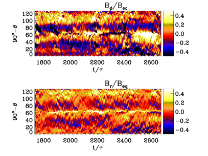
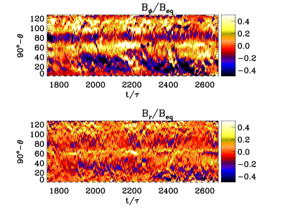
Figure 1: Variation of $\overline{B}_{\phi}$ and $\overline{B}_{r}$ in the convection zone at $r=0.89R$ (left panel) and $r=0.79R$ (right). Dark blue shades represent negative and light yellow positive values. The dotted horizontal lines show the location of the equator at $\theta=\pi/2$. The magnetic field is normalized by the equipartition value.

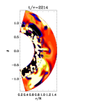
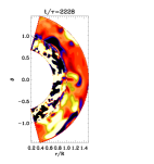
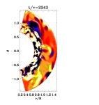
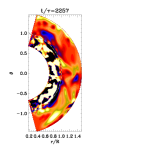
Figure 2: Time series of coronal ejections in spherical coordinates. The normalized current helicity, $\mu_{0}R\,\overline{\mbox{\boldmath$J$}{}\cdot\mbox{\boldmath$B$}{}}/\langle\overline{\mbox{\boldmath$B$}{}^{2}}\rangle_{t}$, is shown in a color-scale representation from different times; dark blue represents negative and light yellow positive values. The dashed horizontal lines show the location of the surface at $r=R$.

The magnetic field emerges through the surface and is ejected as isolated structures. The dynamical evolution is clearly seen in the sequence of images of Figure 2, where the normalized current helicity ($\mu_{0}R\,\overline{\mbox{\boldmath$J$}{}\cdot\mbox{\boldmath$B$}{}}/\langle\overline{\mbox{\boldmath$B$}{}^{2}}\rangle_{t}$) is shown. If one focuses on the region near the equator ($\theta=\pi/2$), a small yellow (i.e. positive) feature with a blue (negative) arch emerges through the surface to the outer atmosphere, where it leaves the domain through the outer boundary. This ejection does not occur as a single event—it rather shows recurrent behavior. We do not, however, find a clear periodicity in the ejection recurrence, like in earlier work. Even though the ejected structures are much smaller than in Warnecke et al. (2011), their shape is similar. However, the detection of an ejection with the aid of the current helicity is much more difficult in convection-driven simulations than in forced turbulence. In Figure 2, one can see large structures diffusing through the surface into the upper atmosphere at higher latitudes. These structures disturb the emergence of ejections and hamper their detection. These larger diffusive structures are also visible in Figure 3, where the normalized current density is averaged over two narrow latitude bands on each hemisphere. The formation of these diffuse structures in the corona seem to get suppressed when the stratification of the system is increased. Nevertheless, ejections are still visible, for example around $t/\tau=1900$, $t/\tau=2200$ (see Figure 2) and $t/\tau=2400$.

The hemispheric rule, as we have found in earlier work, is not completely valid in the current work. The current helicity in Figure 3 shows a different behavior in the northern and southern hemispheres, but one cannot tell clearly the leading sign. This has to do with the much lower values of relative kinetic helicity $h_{\rm rel}(r,t)=\langle\mbox{\boldmath$\omega$}{}\cdot\mbox{\boldmath$u$}{}\rangle/\omega_{\rm rms}u_{\rm rms}$ in the convection simulations. Values of up to $h_{\rm rel}=\mp 0.4$ are reached at some radii in the two hemispheres. In the forced turbulence simulations of our earlier work, we studied purely helical systems with nearly $h_{\rm rel}=\mp 1$.

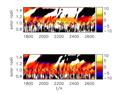
Figure 3: Dependence of the dimensionless ratio $\mu_{0}R\,\overline{\mbox{\boldmath$J$}{}\cdot\mbox{\boldmath$B$}{}}/\langle\overline{\mbox{\boldmath$B$}{}^{2}}\rangle_{t}$ on time $t/\tau$ and radius $r$ in terms of the solar radius. The top panels show a narrow band in $\theta$ in the northern hemisphere and the bottom ones in the southern hemisphere. We have also averaged in latitude from $4.1^{\circ}$ to $19.5^{\circ}$ (left panel) and $32.5^{\circ}$ to $45.5^{\circ}$ (right). Dark blue shades represent negative and light yellow positive values. The dotted horizontal lines show the location of the surface at $r=R$.

In summary, we are able to advance our two-layer model approach by including self-consistent convection, which generates the magnetic field and eventually drives ejections. Not surprisingly, the ejections occur non-periodically and as smaller structures than in earlier work, but this behavior seems to be similar to the Sun. Furthermore, detailed investigations covering a wider range of magnetic and kinetic Reynolds number as well as rotation rates show promising results.

References

- [] Blackman, E. G., & Brandenburg, A. 2003, ApJ, 584, L99
- [] Käpylä, P. J.,Korpi, M. J., Brandenburg, A., Mitra, D. & Tavakol, R. 2010, AN, 331, 73
- [] Käpylä, P. J.,Korpi, M. J., Guerrero, G., Brandenburg, A. & Chatterjee, P. 2011, A&A, 531, A162
- [] Mitra, D., Tavakol, R., Brandenburg, A., & Moss, D. 2009, ApJ, 697, 923
- [] Warnecke, J., & Brandenburg, A. 2010, A&A, 523, A19
- [] Warnecke, J., Brandenburg, A., & Mitra, D. 2011, A&A, 534, A11