Effective Medium Theory of Filamentous Triangular Lattice

Abstract

We present an effective medium theory that includes bending as well as stretching forces, and we use it to calculate mechanical response of a diluted filamentous triangular lattice. In this lattice, bonds are central-force springs, and there are bending forces between neighboring bonds on the same filament. We investigate the diluted lattice in which each bond is present with a probability $p$. We find a rigidity threshold $p_{\textrm{b}}$ which has the same value for all positive bending rigidity and a crossover characterizing bending-, stretching-, and bend-stretch coupled elastic regimes controlled by the central-force rigidity percolation point at $p_{\textrm{CF}}\simeq 2/3$ of the lattice when fiber bending rigidity vanishes.

I Introduction

Random elastic networks provide attractive and realistic models for the mechanical properties of materials as diverse as randomly packed spheres Liu and Nagel (1998); Wyart (2005); Liu and Nagel (2010), network glasses Phillips (1981); Thorpe (1983); Phillips and Thorpe (1985); He and Thorpe (1985); Thorpe et al. (2000), and biopolymer gels Elson (1988); Kasza et al. (2007); Alberts et al. (2008); Janmey et al. (1997); MacKintosh et al. (1995); Head et al. (2003); Wilhelm and Frey (2003); Head et al. (2005); Storm et al. (2005); Onck et al. (2005); Huisman et al. (2007); Huisman and Lubensky (2010). In their simplest form, these networks consist of nodes connected by central-force (CF) springs to on average of $z$ neighbors. They become more rigid as $z$ increases, and they typically exhibit a CF rigidity percolation transition Feng and Sen (1984); Feng et al. (1984); Jacobs and Thorpe (1995) from floppy clusters to a sample spanning-cluster endowed with nonvanishing shear and bulk moduli at a threshold $z=z_{\textrm{CF}}$ very close to the Maxwell isostatic limit Maxwell (1864); Calladine (1978) of $2d$, where $d$ is the spatial dimension, at which the number of constraints imposed by the springs equals the number of degrees of freedom of individual nodes. Generalized versions of these networks, appropriate for the description of network glasses Phillips (1981); Thorpe (1983) and biopolymer gels MacKintosh et al. (1995); Head et al. (2003); Wilhelm and Frey (2003), include bending forces favoring a particular angle between bonds (springs) incident on a given node. For a given value of $z$, networks with bending forces are more rigid than their CF-only counterparts, and they exhibit a rigidity transition at $z=z_{\textrm{b}}<z_{\textrm{CF}}$.

Though numerical calculations, including the pebble game Jacobs and Thorpe (1995, 1996), have provided much of our knowledge about the properties of random elastic networks, effective medium theories (EMTs) Soven (1969); Elliott et al. (1974); Feng et al. (1985); Garboczi and Thorpe (1985); Schwartz et al. (1985) have provided complementary analytical descriptions of CF networks that are simple and at minimum qualitatively correct. EMTs Das et al. (2007); Heussinger and Frey (2006); Heussinger et al. (2007); Broedersz et al. (2011); Das et al. (2012) and heuristic approaches Wyart et al. (2008) that describe both bending and stretching forces have only recently been developed. Here we present details of the derivation of a bend-stretch EMT introduced in Ref. Broedersz et al. (2011) and its application to a bond diluted triangular lattice, whose maximum coordination number is $z_{\rm max}=6$. This lattice has bending and stretching forces modeled on those of biopolymer networks of filamentous semi-flexible polymers, characterized by one-dimensional stretching and bending moduli $\mu$ and $\kappa$ MacKintosh et al. (1995); Head et al. (2003); Wilhelm and Frey (2003), respectively. Our EMT calculates the effective medium moduli $\mu_{m}$ and $\kappa_{m}$ as a function of $\mu$ and $\kappa$ and the probability $p=z/6$ that a bond is occupied. Both the EMT bulk and shear moduli are proportional to $\mu_{m}$. When $\kappa=0$, our EMT reduces to that considered by others Feng et al. (1985); Garboczi and Thorpe (1985) and successfully predicts a second-order CF rigidity threshold at $z_{\textrm{CF}}\simeq 4<z_{\rm max}$ ($p_{\textrm{CF}}=2/3$ in EMT and of order $0.64$ to $0.65$ under various numerical estimates Sahimi (1998); Wang et al. (1992); Broedersz et al. (2011) ) with $\mu_{m}$ increasing linearly in $p-p_{\textrm{CF}}$ near $p_{\textrm{CF}}$ and approaching the undiluted triangular-lattice value of $\mu$ at $p=1$. When bending forces are introduced, our EMT predicts a second-order rigidity threshold $p_{b}<p_{CF}$ for all $\kappa>0$. This qualitatively agrees with the results of an alternative EMT in Ref. Das et al. (2012), although our theory predicts $p_{b}\simeq 0.56$ in poorer agreement with the value $p_{b}\simeq 0.44$ obtained in simulations than the value $p_{b}\simeq 0.457$ predicted there. Near $p_{b}$ we find that $\mu_{m}\sim\kappa(p-p_{\textrm{b}})$ for $\kappa/(\mu a^{2})\ll c_{1}\approx 0.1$ and $\mu_{m}\sim\mu(p-p_{\textrm{b}})$ for $\kappa/(\mu a^{2})\gg c_{1}$, where $a$ is the lattice spacing. Near $p_{\textrm{CF}}$, $\kappa$ is a relevant variable moving the system away from the CF rigidity critical point to a broad crossover regime Wyart et al. (2008); Broedersz et al. (2011) in which $\mu_{m}\sim\kappa^{1/2}\mu^{1/2}$ as shown in the phase diagram of Fig. 1. This crossover is analogous to that for the macroscopic conductivity in a resistor network in which bonds are occupied with resistors with conductance $\sigma_{>}$ with probability $p$ and with conductance $\sigma_{<}<\sigma_{>}$ with probability $1-p$ Straley (1976).

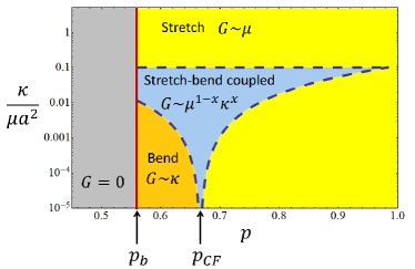
Figure 1: (Color online) Phase diagram of the diluted filamentous triangular lattice showing the central-force and bending rigidity thresholds, respectively, at $p=p_{\textrm{CF}}$ and $p=p_{\textrm{b}}$, the bending-dominated regime at small $\kappa$ in the vicinity of $p_{\textrm{b}}$, the crossover bend-stretch regime near $p_{\textrm{CF}}$, and the stretching dominated regime at large $\kappa$. (Adapted from Ref. Broedersz et al. (2011))

Though the model we study has both stretching and bending forces, it differs in important ways from previously studied models for network glasses Phillips (1981); Thorpe (1983); Phillips and Thorpe (1985); He and Thorpe (1985); Thorpe et al. (2000) and for filamentous gels MacKintosh et al. (1995); Head et al. (2003); Wilhelm and Frey (2003); Head et al. (2005); Storm et al. (2005); Onck et al. (2005); Huisman et al. (2007); Huisman and Lubensky (2010). The maximum coordination number for both of these systems is less than or equal $2d$, and thus neither has a CF rigidity transition for $p<1$ when there are no bending forces. As a result neither exhibits the bend-stretch crossover region near $p_{\textrm{CF}}$ that our model exhibits. Network glasses are well modeled by a randomly diluted four-fold coordinated diamond lattice in which there is a bending-energy cost, characterized by a bending modulus $\kappa$, if the angle between any pair of bonds incident on a site deviates from the tetrahedral angle of $109.5\deg$. The architecture of the undiluted diamond lattice (with $z_{\rm max}=4<2d=6$) is such that its shear modulus vanishes linearly with $\kappa$ He and Thorpe (1985) and elastic response is nonaffine. When diluted, it exhibits a second-order rigidity transition from a state with bending-dominated nonaffine shear response to a state with no rigidity. As dilution decreases, rigidity is still controlled by $\kappa$, but response becomes less nonaffine.

Filamentous networks in two-dimensions are often described by the Mikado model Head et al. (2003); Wilhelm and Frey (2003); Head et al. (2005) in which semi-flexible filaments of a given length $L$ are deposited with random center-of-mass position and random orientation on a two-dimensional plane and in which the points where two filaments cross are joined in frictionless crosslinks. As in our model, there is no energy cost for the relative rotation of two rods about a crosslink, but there is an energy cost for bending the rods at crosslinks. This model is characterized by the ratio $\eta\equiv L/l_{c}$ of the filament length $L$ to the average mesh size, i.e., the average crosslink separation $l_{c}>a$ along a filament, where $a$ is the shortest distance between crosslinks. In the limit $\eta\to\infty$, all filaments traverse the sample, and the system has finite, $\kappa$-independent shear and bulk moduli: There is effectively a CF rigidity transition at $z=4$ when $\eta$ is decreased from infinity. There is a transition at $\eta=\eta_{c}\approx 5.9$ from a floppy to a rigid state with nonaffine response Head et al. (2003); Latva-Kokko and Timonen (2001), and there is a wide crossover region between $\eta=\eta_{c}$ and $\eta=\infty$ in which the shear modulus changes from being bend dominated, nonaffine, and nearly independent of $\mu$ at small $\eta$ to being stretch dominated, nearly affine, and nearly independent of $\kappa$ at large $\eta$. Our EMT applied to the kagome lattice Mao et al. (2011), whose maximum coordination number like that of the Mikado model is four, captures these crossovers. Interestingly, $3d$ lattices composed of straight filaments with $z_{\rm max}=4$ exhibit similar behavior Stenull and Lubensky (2011). When filaments are bent, however, elastic response in one case at least Huisman and Lubensky (2010) is more like that of the diluted diamond lattice with the shear modulus vanishing with $\kappa$ even at at large $L/l_{c}$ or $z$ near $4$.

External tensile stress (i.e., negative pressure) can cause a floppy lattice to become rigid Alexander (1998). Random internal stresses can do so as well in a phenomenon called tensegrity Calladine (1978). Thus a lattice with internal stresses may have a lower rigidity threshold than the same lattice with out internal stresses Huisman and Lubensky (2010). Systems such as network glasses can exhibit two rigidity transitions Thorpe et al. (2000); Boolchand et al. (2005): a second-order transition from a floppy to a rigid but unstressed state followed closely by a first-order transition to a rigid but stressed state. These effects are beyond the scope of EMT and will not be treated.

The outline of our paper is as follows. Section II reviews properties of semi-flexible polymers and defines our model for the harmonic elasticity of crosslinked semi-flexible polymers on a triangular lattice; Sec. III sets up our effective medium theory; Sec. IV presents the results of this theory; and Sec. V compares our EMT with other versions of bend-stretch EMTs and summarizes our results. There are four appendices: App. A derives the energy, which is critical to our version of EMT, of a composite bent rod, App. B presents the detailed form of the dynamical matrix, and App. C provides a detailed comparison of our EMT and that of Refs. Das et al. (2007, 2012).

II Filamentous Polymers on a Triangular Lattice

II.1 Elastic Rods: Continuum and Discretized Energies

Following previous work Head et al. (2003); Wilhelm and Frey (2003), we model individual filaments as homogeneous elastic rods characterized by a stretching (or Young’s) modulus $\mu$ and a bending modulus $\kappa$. We restrict out attention to two dimensions. The filament energy is thus,

$$E=\frac{1}{2}\int_{0}^{L}ds\left[\mu\left(\frac{du(s)}{ds}\right)^{2}+\kappa\left(\frac{d\theta(s)}{ds}\right)^{2}\right],$$ (1)

where $s$ is the arclength coordinate, $L$ is the unstretched contour length of the polymer, and $u(s)$ and $\theta(s)$ are, respectively, the longitudinal displacement and angle of the unit tangent to the polymer at $s$. We treat this as a purely mechanical model in which $\mu$ and $\kappa$ are fixed, and we do not consider the entropic contributions to the energy that arise from thermally induced transverse fluctuations of the filaments MacKintosh et al. (1995); Marko and Siggia (1995); Storm et al. (2005). Three length scales can be identified in this elastic energy. The first is the contour length of the polymers, $L$. The second, $l_{\textrm{bend}}\equiv\sqrt{\kappa/\mu}$, characterizes the relative strength of stretching and bending. For an elastic rod made of a homogeneous material, $l_{\textrm{bend}}$ is simply proportional to the radius of the rod. A third length, the mesh size $l_{c}$ characterizing the connectivity of the network, can be identified for crosslinked polymer networks. The ratio $L/l_{c}$ is a measure of the connectivity of the lattice. Finite filaments of length $L$ with this energy act like springs with stretching spring constant $k_{||}=\mu/L$ and bending constant $\kappa/L^{3}$.

In order to develop a model of crosslinked filaments on a lattice with a random distribution of stretching and bending moduli of the sort that we will encounter in our EMTs, we need first to develop a discretized form of the continuum beam energy [Eq. (1)] with inhomogeneous stretching and bending moduli. We begin by dividing a filament of length $L$ into $N$ segments (bonds) of length $a$, labeled $i=1,\cdots,N$ and terminated by nodes (sites) $i=0\cdots N$. In equilibrium in the absence of external forces, the filament is straight, and node $i$ is at position $s_{i}=ia$ while that of the center of bond $i$, which lies between sites nodes $i-1$ and $i$, is at position $s_{i}-(a/2)$ as shown in Fig. 2. Individual stretching and bending moduli $\mu_{i}$ and $\kappa_{i}$ are associated with bond $i$ as shown in Fig. 2. Individual stretching an bending moduli $\mu_{i}$ and $\kappa_{i}$ are associated with bond $i$.

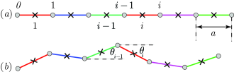
Figure 2: (color online) Schematic of a filament of length $5a$ divided into $5$ segments of length $a$ (a) in the equilibrium configuration and (b) in a distorted configuration. Circles mark lattice nodes (located as positions $ia$), and crosses mark the centers of bonds located at positions $[i-(1/2)]a$. The different colors of the bonds indicate different values for the stretching and bending moduli. The angle of the bonds $i-1$ and $i$ are indicated in (b). In the limit of slow changes in $\theta_{i}$, the slope of the $h(s)\equiv u^{\perp}(s)$ is constant in bond $i$, and bond angle $i$ is the angle of the line connecting connecting site $i-1$ with site $i$ for small $\theta_{i}$.

The derivation of the discretized stretching energy is straightforward: Associated with each node $i$ is a longitudinal displacement $u_{i}^{||}$ and with each bond $i$ an energy

$$E_{i}^{s}=\frac{1}{2}\frac{\mu_{i}}{a}(u_{i+1}^{||}-u_{i}^{||})^{2}.$$ (2)

The total stretching energy of a filament is the sum of these bond energies. The discretized equations of motion arising from this inhomogeneous discrete model agree with those arising from a continuum model in the continuum $a\rightarrow 0$ limit.

The derivation of a discretized bending energy is more subtle. Consider first a homogeneous model in which $\kappa$ is the same in each segment. Here we assign an angle $\theta_{i}$ to each bond, and an energy $(1/2)(\kappa/a^{3})(\theta_{i+1}-\theta_{i})^{2}$ to the node $i$, which lies between bonds $i$ and $i+1$. This energy is, of course, constructed so that in the continuum ($a\rightarrow 0$) limit $(\theta_{i}-\theta_{i-1})/a\rightarrow d\theta/ds$ and the bending part of Eq. (1) is retrieved. This works because the filament segment between the center of bond $i$ [at position $s_{i}a-(a/2)$] and that of bond $i+1$ [at position $s_{i}a+(a/2)$] is uniform with bending modulus $\kappa$, and as a result, the energy of that segment is the bond energy given above. But what happens if the bending moduli in these two segments are different, i.e., $\kappa_{i}\neq\kappa_{j}$? We show in App. A that the energy of a filament segment encompassing half of bond $i$ with bending modulus $\kappa_{i}$ and half of bond $i+1$ with bending modulus $\kappa_{i+1}$ is

$$E_{i,i+1}^{b}=\frac{1}{2}\frac{\overline{\kappa}_{i}}{a^{3}}(\theta_{i+1}-\theta_{i})^{2}$$ (3)

where

$$\overline{\kappa}_{i}=\frac{2\kappa_{i}\kappa_{i+1}}{\kappa_{i}+\kappa_{i+1}},$$ (4)

i.e., the two halves of the bending spring connecting bond $i$ to bond $i+1$ add like springs in series. Note that $\overline{\kappa}_{i}$ satisfies the required limits that it reduce to $\kappa_{i}$ when $\kappa_{i+1}=\kappa_{i}$ and that it vanish if either $\kappa_{i}$ or $\kappa_{i+1}=0$. The total bending energy of a filament is thus

$$E_{\text{fil}}^{b}=\frac{1}{2}\sum_{i=1}^{N}\overline{\kappa}_{i}(\theta_{i+1}-\theta_{i})^{2}.$$ (5)

Minimization of this energy gives a series of difference equations for $\theta_{i}$. We show in App. A that the solution to these equations faithfully reproduces $\theta(s)$ calculated from the continuum equations resulting from the minimization of the continuum bending energy for the particular case of $\kappa$’s having one value for $0<s<s_{1}$ and another value for $s_{1}<s<L$. A generalization of this calculation to more general distributions of $\kappa$ is straightforward and yields the same results for the discrete and continuum models.

Ultimately, we are interested in the positions of the nodes, and we need an expression relating these positions to the bond angles. In the ground state, all of the bonds of the filament are aligned along a common direction specified by a unit vector, $\mathbf{e}$, and the ground-state positions are $\mathbf{r}_{i}=s_{i}\mathbf{e}$. Distortions of the filament are described by the displacement vectors $\mathbf{u}_{i}=u_{i}^{||}\mathbf{e}+u_{i}^{\perp}\mathbf{e}^{\perp}$ where $\mathbf{e}^{\perp}$ is unit vector perpendicular to $\mathbf{e}$. As discussed more fully in App. A, within the linearized theory we use, the angle that bond $i$ makes with $\mathbf{e}$ is then $\theta_{i}=(u_{i}^{\perp}-u_{i-1}^{\perp})/a$. Thus the bending energy $(1/2)\overline{\kappa}_{i}(\theta_{i+1}-\theta_{i})^{2}\approx(1/2)\overline{\kappa}_{i}(2u_{i}^{\perp}-u_{i+1}^{\perp}-u_{i-1}^{\perp})^{2}$ couples the displacements of sites $i-1$, $i$, and $i+1$, and it can be viewed as an interaction defined on a kind of next-nearest-neighbor ($NNN$) connecting sites $i-1$ and $i+1$. This bond, however, only exists if both $NN$ bond $i$ and $i+1$ are occupied. In what follows, we will refer to the bending $NNN$ bonds as phantom bonds since they do not have an independent existence. We will also employ an alternative notation in which a bond connecting nodes $\ell$ and $\ell^{\prime}$ on a lattice will be denoted by $\langle\ell,\ell^{\prime}\rangle$ and the angle that bond makes with the horizontal axis by $\theta_{\langle\ell,\ell^{\prime}\rangle}$. The $NNN$ bending energy is then $(1/2)\kappa(\theta_{\ell,\ell^{\prime},\ell^{\prime\prime}})^{2}$, where $\theta_{\ell,\ell^{\prime},\ell"}=\theta_{\langle\ell,\ell^{\prime}\rangle}-\theta_{\langle\ell^{\prime},\ell^{\prime\prime}\rangle}$ with the understanding that sties $\ell$, $\ell^{\prime}$, and $\ell^{\prime\prime}$ all lie on a single filament.

II.2 Triangular lattice of filamentous polymers

To create a network of crosslinked semiflexible polymers we randomly remove bonds on a triangular lattice. Polymers correspond to lines of connected, occupied colinear bonds, and crosslinks correspond to sites at which two or three polymers cross. Each bond in the lattice can be assigned one of the three directions designated by the unit vectors $\mathbf{e}_{n}$ shown in Fig. 3. All of the bonds in a given filament are aligned along one of these directions and the filament itself is directed. Sites on the lattice are labeled by a two-component index $\ell=(l_{1},l_{2})$, and their equilibrium positions are $\mathbf{r}_{\ell}=a(l_{1}\mathbf{e}_{1}+l_{2}\mathbf{e}_{2})$. We adopt the convention that $NN$ bonds $\langle\ell,\ell^{\prime}\rangle$ connect sites with equilibrium positions $\mathbf{r}_{\ell}$ and $\mathbf{r}_{\ell^{\prime}}=\mathbf{r}_{\ell}+a\mathbf{e}_{n}$ for one of the directions $\mathbf{e}_{n}$. Upon distortion, the position of site $\ell$ changes to $\mathbf{R}_{\ell}=\mathbf{r}_{\ell}+\mathbf{u}_{\ell}$, where $\mathbf{u}_{\ell}$ is the displacement vector of site $\ell$. We define all bond angles to be zero in the undistorted lattice. In the distorted lattice, the angle of bond $\langle\ell,\ell^{\prime}\rangle$ becomes $\theta_{\langle\ell,\ell^{\prime}\rangle}\approx\mathbf{u}_{\ell,\ell^{\prime}}\cdot\hat{\mathbf{r}}_{\ell,\ell^{\prime}}^{\perp}/a$, where $\mathbf{u}_{\ell,\ell^{\prime}}=\mathbf{u}_{\ell^{\prime}}-\mathbf{u}_{\ell}$ and $\hat{\mathbf{r}}_{\ell,\ell^{\prime}}^{\perp}$ is the unit vector perpendicular to the bond direction along $\mathbf{r}_{\ell^{\prime}}-\mathbf{r}_{\ell}$ and is equal to one of the unit vectors $\mathbf{e}^{\perp}_{n}$ perpendicular to $\mathbf{e}_{n}$. We now assign stretching energies to each bond and bending energies to each phantom $NNN$ bond along a lattice direction in accordance with the discretized energy of an individual filament [Eqs. (2) and (3)] to obtain the harmonic energy on a diluted lattice

$$E = E_{s}+E_{b}$$ (6a)

$$E_{s} = \frac{1}{2}\frac{\mu}{a}\sum_{\langle\ell,\ell^{\prime}\rangle}g_{\ell,\ell^{\prime}}(\mathbf{u}_{\ell\ell^{\prime}}\cdot\hat{\mathbf{r}}_{\ell\ell^{\prime}})^{2},$$ (6b)

$$E_{b} = \frac{1}{2}\frac{\kappa}{a}\sum_{\ell^{\prime},n}g_{\ell,\ell^{\prime}}g_{\ell^{\prime},\ell^{\prime\prime}}(\theta_{\ell\ell^{\prime}\ell^{\prime\prime}})^{2}$$

$$= \frac{1}{2}\frac{\kappa}{a^{3}}\sum_{\langle\ell,\ell^{\prime},\ell^{\prime\prime}\rangle}g_{\ell,\ell^{\prime}}g_{\ell^{\prime},\ell^{\prime\prime}}\big{[}(\mathbf{u}_{\ell\ell^{\prime}}-\mathbf{u}_{\ell^{\prime}\ell^{\prime\prime}})\cdot\hat{\mathbf{r}}_{\ell,\ell^{\prime}}^{\perp}\big{]}^{2},$$

where $g_{\ell,\ell^{\prime}}=1$ if the bond $\langle\ell,\ell^{\prime}\rangle$ is occupied and $g_{\ell,\ell^{\prime}}=0$ if it is not. This is the model was introduced in references Wilhelm and Frey (2003) and Head et al. (2005) in their study of the Mikado model. A version of this model in which there is a bond-angle energy between all pairs of bonds sharing a common site rather than only between pairs of parallel bonds was introduced earlier in reference Feng et al. (1984).

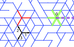
Figure 3: (color online) Filamentous triangular lattice with bonds randomly occupied with probability $p$. The unit vectors $\mathbf{e}_{1}$, $\mathbf{e}_{2}$, $\mathbf{e}_{3}$ are marked by “1, 2, 3”, the 3 stretch energy vectors $\mathbf{B}^{s}_{n}$ are marked by the 3 red single lines, and the 3 bending energy vectors $\mathbf{B}^{b}_{n}$ are marked by the 3 green double lines. The purple dashed double line marks the bending vector $\mathbf{B}^{b}_{4}$ if the origin is marked by $0$.

When $p=1$, all bonds are occupied and $E$ becomes homogeneous. In this limit, the long-wavelength elastic energy reduces to the elastic energy of an isotropic $2d$ medium,

$$E=\int d^{2}x\left[\frac{\bar{\lambda}}{2}\big{(}\textrm{Tr}\underline{\underline{u}}\big{)}^{2}+\bar{\mu}\textrm{Tr}\underline{\underline{u}}^{2}\right],$$ (7)

where $\underline{\underline{u}}$ is the linearized symmetric Cauchy strain tensor with Cartesian components $u_{ij}$, $\bar{\lambda}$ and $\bar{\mu}$ are the Lamé coefficients, $\bar{\lambda}=\bar{\mu}=(\sqrt{3}/4)(\mu/a)$, which depend only on $\mu$ and not on $\kappa$. $\bar{\mu}$ is the macroscopic shear modulus. The bending constant $\kappa$ only appears in the higher-order gradients of the the displacement vector. Upon dilution, each of the bonds is present with a probability $p$, and the resulting lattice corresponds to a random network of semiflexible filaments of finite random lengths $L$, whose average as a function of $p$ is $\langle L\rangle=a/(1-p)$ Broedersz et al. (2011). It is a straightforward exercise to show that the average distance $l_{c}$ between crosslinks (i.e. nodes with at which two or more filaments cross) differs by at most a factor of $2$ from $a$, and we will use treat them as the same quantity in what follows. In EMT, $\mu$ is replaced in diluted samples by its effective medium value $\mu_{m}$, and the macroscopic EMT shear modulus of these samples is

$$G=(\sqrt{3}/4)(\mu_{m}/a).$$ (8)

In the undiluted limit the shear modulus is $G_{0}=(\sqrt{3}/4)(\mu/a)$, and $G/G_{0}=\mu_{m}/\mu$. Because our calculations are centered on the evaluation of $\mu_{m}$ rather than $G$, we will in what follows use $\mu_{m}$ as a proxy for $G$, reminding the reader where appropriate of this simple relation between the effective medium parameter and $G$.

III Effective Medium Theory

We study the elasticity of our network using an effective-medium approximation Soven (1969); Elliott et al. (1974) in which the random inhomogeneous system is replaced with an effective homogeneous one constructed so that the average scattering from a bond (or chosen set of bonds) with the probability distribution of the original random lattice vanishes. In more technical terms, the effective medium is chosen so that average $T$-matrix associated with the bond vanishes. This approximation has been shown to be a powerful tool for the calculation of properties of random systems, from the electronic structure of alloys Soven (1969); Kirkpatrick et al. (1970) to the elasticity of random networks Feng et al. (1985); Mao et al. (2010).

Our elastic energy is a bilinear form in the $2N$-dimensional displacement vector $\mathbf{u}$ determined by the $2N\times 2N$ dynamical matrix $\mathbf{D}$, where $N$ is the number of sites in the lattice. We will represent these two quantities in both the lattice basis and the wavenumber basis where the components of $\mathbf{u}$ are, respectively, the $2$-dimensional vectors $\mathbf{u}_{\ell}$ and $\mathbf{u}_{\mathbf{q}}$ for each of the $N$ lattice positions $\ell$ or wavenumbers $\mathbf{q}$ and the components of $\mathbf{D}$ are respectively the $2\times 2$ matrices $\mathbf{D}_{\ell,\ell^{\prime}}$ and $\mathbf{D}_{\mathbf{q},\mathbf{q}^{\prime}}$ for each pair $(\ell,\ell^{\prime})$ or $(\mathbf{q},\mathbf{q}^{\prime})$. We use the convention in which arbitrary vectors $\mathbf{v}$ or matrices $\mathbf{M}$ in the two bases are related via

$$\mathbf{v}_{\mathbf{q}} =\sum_{\ell}\mathbf{v}_{\ell}e^{-i\mathbf{q}\cdot\mathbf{r}_{\ell}},\qquad\mathbf{v}_{\ell}=\frac{1}{N}\sum_{\mathbf{q}}\mathbf{v}_{\mathbf{q}}e^{i\mathbf{q}\cdot\mathbf{r}_{\ell}},$$ (9)

$$\mathbf{D}_{\mathbf{q},\mathbf{q}^{\prime}} =\sum_{\ell,\ell^{\prime}}e^{-i\mathbf{q}\cdot\mathbf{r}_{\ell}}\mathbf{D}_{\ell,\ell^{\prime}}e^{i\mathbf{q}^{\prime}\cdot\mathbf{r}_{\ell^{\prime}}},$$

$$\mathbf{D}_{\ell,\ell^{\prime}} =\frac{1}{N^{2}}\sum_{\mathbf{q},\mathbf{q}^{\prime}}e^{i\mathbf{q}\cdot\mathbf{r}_{\ell}}\mathbf{D}_{\mathbf{q},\mathbf{q}^{\prime}}e^{-i\mathbf{q}^{\prime}\cdot\mathbf{r}_{\ell^{\prime}}}.$$ (10)

The elastic energy is thus

$$E=\frac{1}{2}\mathbf{u}\cdot\mathbf{D}\cdot\mathbf{u}$$

$$=\frac{1}{2}\sum_{\ell,\ell^{\prime}}\mathbf{u}_{\ell}\cdot\mathbf{D}_{\ell,\ell^{\prime}}\cdot\mathbf{u}_{\ell^{\prime}}=\frac{1}{2N^{2}}\sum_{\mathbf{q},\mathbf{q}^{\prime}}\mathbf{u}_{-\mathbf{q}}\cdot\mathbf{D}_{\mathbf{q},\mathbf{q}^{\prime}}\cdot\mathbf{u}_{\mathbf{q}^{\prime}},$$ (11)

where here and in the following the “dot” signifies the multiplication of a matrix and a vector or of two matrices. The zero-frequency phonon Green’s function (which is a $2N\times 2N$ matrix) is minus the inverse of the dynamical matrix:

$$\mathbf{G}=-\mathbf{D}^{-1}.$$ (12)

In EMT, the inhomogeneous and random dynamical matrix $\mathbf{D}$ is replaced by a homogeneous, translationally invariant one $\mathbf{D}^{(m)}$, with $\mathbf{D}^{(m)}_{\ell,\ell^{\prime}}=\mathbf{D}^{(m)}_{\ell-\ell^{\prime}}$ and

$$\mathbf{D}^{(m)}_{\mathbf{q},\mathbf{q}^{\prime}}=N\delta_{\mathbf{q},\mathbf{q}^{\prime}}\mathbf{D}^{(m)}_{\mathbf{q}},$$ (13)

along with a perturbation matrix $\mathbf{V}$, which we will specify in detail shortly:

$$\mathbf{D}=\mathbf{D}^{(m)}+\mathbf{V}=-(\mathbf{G}^{(m)})^{-1}+\mathbf{V}=-\mathbf{G}^{-1},$$ (14)

where the superscript $(m)$ stands for “effective medium”. The full Green’s function can thus be expressed as

$$\mathbf{G}=((\mathbf{G}^{(m)})^{-1}-\mathbf{V})^{-1}=\mathbf{G}^{(m)}+\mathbf{G}^{(m)}\cdot\mathbf{T}\cdot\mathbf{G}^{(m)},$$ (15)

where $\mathbf{T}$ is the $T$-matrix describing the scattering resulting from $\mathbf{V}$:

$$\mathbf{T} = \mathbf{V}\cdot(\mathbf{I}-\mathbf{V}\cdot\mathbf{G}^{(m)})^{-1}=(\mathbf{I}-\mathbf{V}\cdot\mathbf{G}^{(m)}))^{-1}\cdot\mathbf{V}$$ (16)

$$= \mathbf{V}+\mathbf{V}\cdot\mathbf{G}^{(m)}\cdot\mathbf{V}+\cdots.$$

This expresses the $T$-matrix in general form. Our next step is to specify both $\mathbf{D}^{(m)}$ and $\mathbf{V}$.

We begin with $\mathbf{D}^{(m)}$. Normally, the effective-medium elastic energy would simply be the random one of Eq. (6) with $\mu$ and $\kappa$ replaced by their respective effective-medium values $\mu_{m}$ and $\kappa_{m}$ and $g_{\ell,\ell^{\prime}}$ replaced by one. It turns out, however, as we will shortly demonstrate, that the effective-medium equations, determined by setting the average $T$-matrix equal to zero, consists of three independent equations whose solutions requires three independent parameters. If the above simple procedure for constructing the effective-medium energy is followed, there are only two parameters, $\mu_{m}$ and $\kappa_{m}$, and to solve the EMT equations, it is necessary to introduce a new term to this energy with a new parameter, which we denote by $\lambda_{m}$. This additional energy, whose form is dictated, as we shall see, by the EMT equations, couples angles on neighboring $NNN$ phantom bonds:

$$E_{bb}(\lambda_{m})=\frac{\lambda_{m}}{a^{3}}\sum_{\ell_{2}}\theta_{\ell_{1},\ell_{2},\ell_{3}}\theta_{\ell_{2},\ell_{3},\ell_{4}},$$ (17)

where it is understood that the sites $\ell_{,}\ell_{2},\ell_{3},\ell_{4}$ are sequential sites along a filament as shown in Fig. 4. The total effective-medium energy is thus

$$E^{(m)}(\mu_{m},\kappa_{m},\lambda_{m})=E_{s}(\mu_{m})+E_{b}(\kappa_{m})+E_{bb}(\lambda_{m}),$$ (18)

and its associated dynamical matrix is

$$\mathbf{D}^{(m)}_{\mathbf{q}}(\mu_{m},\kappa_{m})=\frac{\mu_{m}}{a}\sum_{n=1}^{3}\mathbf{B}^{s}_{n,\mathbf{q}}\mathbf{B}^{s}_{n,-\mathbf{q}}$$

$$+\frac{\kappa_{m}}{a^{3}}\sum_{n=1}^{3}\mathbf{B}^{b}_{n,\mathbf{q}}\mathbf{B}^{b}_{n,-\mathbf{q}}+\frac{\lambda_{m}}{a^{3}}\sum_{m=1}^{3}2\cos(\mathbf{q}\cdot\mathbf{e}_{m})\mathbf{B}^{b}_{m,\mathbf{q}}\mathbf{B}^{b}_{m,-\mathbf{q}}$$ (19)

where

$$\mathbf{B}^{s}_{n,\mathbf{q}} = (1-e^{-i\mathbf{q}\cdot\mathbf{e}_{n}})\mathbf{e}_{n},$$ (20a)

$$\mathbf{B}^{b}_{n,\mathbf{q}} = 2[1-\cos(\mathbf{q}\cdot\mathbf{e}_{n})]\mathbf{e}^{\perp}_{n},$$ (20b)

are two-dimensional vectors and where a simplified notation is used in which two of these vectors in a row denotes a direct product creating a $2\times 2$ matrix.

The perturbation $\mathbf{V}$ arises from the removal of a single bond, whose endpoints, $\ell_{2}$ and $\ell_{3}$, we take to be contiguous sites along a filament parallel to the $\mathbf{e}_{1}$ axis with $\ell_{2}$ located at the origin and $\ell_{3}$ at position $\mathbf{e}_{1}$. If there is no bending energy (i.e., $\kappa=0$), the energy of this bond relative to the effective medium is thus

$$E_{V}^{s}=\frac{1}{2}\frac{\mu_{s}-\mu_{m}}{a}[(\mathbf{u}_{\ell_{2}}-\mathbf{u}_{\ell_{3}})\cdot\mathbf{e}_{1}]^{2},$$ (21)

where $\mu_{s}=\mu g_{\ell_{2},\ell_{3}}$ so that its probability distribution is

$$P(\mu_{s})=p\delta(\mu_{s}-\mu)+(1-p)\delta(\mu_{s}).$$ (22)

This bond stretching energy defines $\mathbf{V}^{s}$:

$$\mathbf{V}_{\mathbf{q},\mathbf{q}^{\prime}}^{s}=a^{-1}(\mu_{s}-\mu_{m})\mathbf{B}^{s}_{1,\mathbf{q}}\mathbf{B}^{s}_{1,-\mathbf{q}^{\prime}}.$$ (23)

Note that $\mathbf{V}_{\mathbf{q},\mathbf{q}^{\prime}}^{s}$ factorizes into a product of a term depending only on $\mathbf{q}$ and a term depending only on $\mathbf{q}^{\prime}$. This is a property, shared by the other contributions to $\mathbf{V}$, that, as we shall see, makes the calculation of the $T$-matrix from Eq. (16) tractable.

Replacing bond $\langle\ell_{2},\ell_{3}\rangle$ changes the bending as well as the stretching modulus of that bond. As discussed in Sec. II and App. A, this leads to a change in the bending constant of the $NNN$ bonds $\langle\ell_{1},\ell_{2},\ell_{3}\rangle$ and $\langle\ell_{2},\ell_{3},\ell_{4}\rangle$ that share the replaced bond $\langle\ell_{2},\ell_{3}\rangle$ along a filament from $\kappa_{m}$ to

$$\kappa_{c}=2\Big{(}\frac{1}{\kappa_{s}}+\frac{1}{\kappa_{m}}\Big{)}^{-1},$$ (24)

where $\kappa_{s}\equiv\kappa g_{\ell_{2},\ell_{3}}$ equals zero if the bond $\langle\ell_{2}\ell_{3}\rangle$ is vacant and $\kappa$ if it is occupied. The probability distribution for $\kappa_{s}$ is thus

$$P(\kappa_{s})=p\delta(\kappa_{s}-\kappa)+(1-p)\delta(\kappa_{s}),$$ (25)

and the joint probability distribution for both $\mu_{s}$ and $\kappa_{s}$ is

$$P(\mu_{s},\kappa_{s})=p\delta(\mu_{s}-\mu)\delta(\kappa_{s}-\kappa)+(1-p)\delta(\mu_{s})\delta(\kappa_{s}).$$ (26)

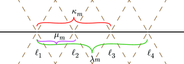
Figure 4: (Color online) Positions of sites $\ell_{1},\ell_{2},\ell_{3},\ell_{4}$, and interactions in the effective medium, including NN stretching term of rigidity $\mu_{m}$, NNN bending term of rigidity $\kappa_{m}$, and third neighbor effective coupling term of rigidity $\lambda_{m}$.

If $\langle\ell_{2}\ell_{3}\rangle$ is occupied $\kappa_{c}=2\kappa\kappa_{m}/(\kappa+\kappa_{m})$ is a nonlinear function of $\kappa$ and $\kappa_{m}$. These considerations determine the bending contribution to $E_{V}$,

$$E_{V}^{b}= \frac{1}{2}\frac{\kappa_{c}(\kappa_{s})-\kappa_{m}}{a^{3}}\left[(\theta_{\ell_{1},\ell_{2},\ell_{3}})^{2}+(\theta_{\ell_{2},\ell_{3},\ell_{4}})^{2}\right]$$

$$= \frac{1}{2}\frac{\kappa_{c}(\kappa_{s})-\kappa_{m}}{a^{3}}\Big{\{}[(2\mathbf{u}_{\ell_{2}}-\mathbf{u}_{\ell_{3}}-\mathbf{u}_{\ell_{1}})\cdot\mathbf{e}^{\perp}_{1}]^{2}$$

$$\quad+[(2\mathbf{u}_{\ell_{3}}-\mathbf{u}_{\ell_{4}}-\mathbf{u}_{\ell_{2}})\cdot\mathbf{e}^{\perp}_{1}]^{2}\Big{\}},$$ (27)

and the bending contribution to $\mathbf{V}$:

$$\mathbf{V}^{b}_{\mathbf{q},\mathbf{q}^{\prime}} = a^{-3}(\kappa_{c}(\kappa_{s})-\kappa_{m})\mathbf{B}^{b}_{1,\mathbf{q}}\mathbf{B}^{b}_{1,-\mathbf{q}^{\prime}}$$ (28)

$$+a^{-3}(\kappa_{c}(\kappa_{s})-\kappa_{m})\mathbf{B}^{b}_{4,\mathbf{q}}\mathbf{B}^{b}_{4,-\mathbf{q}^{\prime}},$$

where the vectors $\mathbf{B}^{b}_{1,\mathbf{q}}$ [Eq. (20b)] and $\mathbf{B}^{b}_{4,\mathbf{q}}\equiv e^{-i\mathbf{q}\cdot\mathbf{e}_{1}}\mathbf{B}^{b}_{1,\mathbf{q}}$ represent the bending of the bond pair connecting sites $\ell_{1},\ell_{2},\ell_{3}$ and $\ell_{2},\ell_{3},\ell_{4}$, respectively. Finally, the original energy had no term corresponding the coupling between $\theta_{\ell_{1},\ell_{2},\ell_{3}}$ and $\theta_{\ell_{2},\ell_{3},\ell_{4}}$ that appears in the effective medium energy [Eq. 17], so that replacement of the bond $\langle\ell_{2},\ell_{3}\rangle$ with its form in the original energy removes the energy associated with that bond in $E^{(m)}$ and creates the contribution

$$\mathbf{V}_{\mathbf{q},\mathbf{q}^{\prime}}^{bb}=-\frac{\lambda_{m}}{a^{3}}[\mathbf{B}^{b}_{1,\mathbf{q}}\mathbf{B}^{b}_{4,-\mathbf{q}^{\prime}}+\mathbf{B}^{b}_{4,\mathbf{q}}\mathbf{B}^{b}_{1,-\mathbf{q}^{\prime}}]$$ (29)

to $\mathbf{V}$. The complete $\mathbf{V}$ is thus $\mathbf{V}=\mathbf{V}^{s}+\mathbf{V}^{b}+\mathbf{V}^{bb}$, which can conveniently be expressed as

$$\mathbf{V}_{\mathbf{q},\mathbf{q}^{\prime}}(\mu_{s},\kappa_{s})=\sum_{\alpha,\beta}\tilde{V}^{\alpha\beta}(\mu_{s},\kappa_{s})\mathbf{B}_{\mathbf{q}}^{\alpha}\mathbf{B}_{-\mathbf{q}}^{\beta},$$ (30)

where $\alpha=\{(s,1),(b,1),(b,4)\}$ labels the three vectors $\{\mathbf{B}^{s}_{1,\mathbf{q}},\mathbf{B}^{b}_{1,\mathbf{q}},\mathbf{B}^{b}_{4,\mathbf{q}}\}$. The scattering potential in this basis is

$$\tilde{V}(\mu_{s},\kappa_{s},\lambda_{m})=\left(\!\begin{array}[]{ccc}(\mu_{s}-\mu_{m})/a&0&0\\ 0&(\kappa_{c}(\kappa_{s})-\kappa_{m})/a^{3}&-\lambda_{m}/a^{3}\\ 0&-\lambda_{m}/a^{3}&(\kappa_{c}(\kappa_{s})-\kappa_{m})/a^{3}\\ \end{array}\!\right),$$ (34)

We are now in a position to calculate the $T$-matrix. Consider first the first non-trivial term in its series expansion [Eq. (16)]:

$$\mathbf{V}\cdot\mathbf{G}\cdot\mathbf{V}\rightarrow \frac{1}{N}\sum_{\mathbf{q}_{1}}\!\mathbf{V}_{\mathbf{q},\mathbf{q}_{1}}\!\!\cdot\!\mathbf{G}_{\mathbf{q}_{1}}^{(m)}\!\!\cdot\!\mathbf{V}_{\mathbf{q}_{1},\mathbf{q}^{\prime}}$$

$$= \sum_{\alpha,\beta,\alpha^{\prime},\beta^{\prime}}\mathbf{B}_{\mathbf{q}}^{\alpha}\tilde{V}^{\alpha\beta}\cdot(\tilde{G}^{(m)})^{\beta\alpha^{\prime}}\cdot\tilde{V}^{\alpha^{\prime}\beta^{\prime}}\mathbf{B}_{-\mathbf{q}^{\prime}}^{\beta^{\prime}}$$ (35)

where $\tilde{G}$ is defined as

$$(\tilde{G}^{(m)})^{\beta,\alpha^{\prime}}\equiv\frac{1}{N}\sum_{\mathbf{q}_{1}}\!\mathbf{B}_{-\mathbf{q}_{1}}^{\beta}\cdot\!\mathbf{G}^{(m)}_{\mathbf{q}_{1}}\!\!\cdot\!\mathbf{B}_{\mathbf{q}_{1}}^{\alpha^{\prime}}.$$ (36)

It is clear that subsequent terms in the Taylor series for $\mathbf{T}$ decompose in a similar way and that

$$\mathbf{T}_{\mathbf{q},\mathbf{q}^{\prime}}=\sum_{\alpha,\beta}\mathbf{B}_{\mathbf{q}}^{\alpha}\tilde{T}^{\alpha\beta}\mathbf{B}_{-\mathbf{q}^{\prime}}^{\beta}$$ (37)

where the $3\times 3$ matrix $\tilde{T}$ satisfies.

$$\tilde{T}=\tilde{V}(\tilde{I}-\tilde{G}^{(m)}\tilde{V})^{-1}=(\tilde{I}-\tilde{V}\tilde{G}^{(m)})^{-1}\tilde{V}=(\tilde{V}^{-1}-\tilde{G})^{-1},$$ (38)

where $\tilde{V}\tilde{G}^{(m)}$ signifies a matrix product.

There are now a couple of points that must be attended to before we present the details or our calculation. First, we show in App. B that $\tilde{G}^{(m)}$ is a symmetric matrix whose $12$ and $13$ components vanish and whose $22$ and $33$ components are equal whether or not $\lambda_{m}$ is zero. Importantly, the $23$ component of $\tilde{G}^{(m)}$ is nonzero even if $\lambda_{m}$ is zero. Thus, $\tilde{G}^{(m)}$ has the same structure as $\tilde{V}$:

$$\tilde{G}^{(m)}=\left(\begin{array}[]{ccc}G^{(m)}_{1}&0&0\\ 0&G^{(m)}_{2}&G^{(m)}_{3}\\ 0&G^{(m)}_{3}&G^{(m)}_{2}\\ \end{array}\right),$$ (42)

where $G^{(m)}_{1}=(\tilde{G}^{(m)})^{11}$, $G^{(m)}_{2}=(\tilde{G}^{(m)})^{22}$, and $G^{(m)}_{3}=(\tilde{G}^{(m)})^{23}$. This implies from Eq. (38) that $\tilde{T}$ also has the same structure as $\tilde{G}^{(m)}$ with three independent components ($\tilde{T}^{11},\tilde{T}^{22}=\tilde{T}^{33}$, and $\tilde{T}^{23}$) even if $\lambda_{m}=0$. Thus, the EMT equation

$$\langle\tilde{T}\rangle=p\tilde{T}(\mu_{s}=\mu,\kappa_{s}=\kappa)+(1-p)\tilde{T}(\mu_{s}=0,\kappa_{s}=0)=0,$$ (43)

reduces to three independent equations whose solution requires three independent parameters. The addition of the energy $E_{bb}^{(m)}$ [Eq. (17)] adds the needed third parameter, $\lambda_{m}$, to $\mu_{m}$ and $\kappa_{m}$ and gives $\tilde{V}$ the same structure as $\tilde{T}$ and and $\tilde{G}$.

To solve Eq. (43), we first write it as

$$p\tilde{V}(\mu,\kappa)[\tilde{I}-\tilde{G}^{(m)}\tilde{V}(\mu,\kappa)]^{-1}$$

$$+(1-p)[\tilde{I}-\tilde{V}(0,0)\tilde{G}^{(m)}]^{-1}\tilde{V}(0,0)=0,$$ (44)

where we used both forms of Eq. (38). Multiplying this equation on the left by $[\tilde{I}-\tilde{G}^{(m)}\tilde{V}(0,0)]^{-1}$ and on the right by $[\tilde{I}-\tilde{V}(\mu,\kappa)\tilde{G}^{(m)}]^{-1}$, we obtain

$$p\tilde{V}(\mu,\kappa)+(1-p)\tilde{V}(0,0)-\tilde{V}(0,0)\tilde{G}^{(m)}\tilde{V}(\mu,\kappa)=0,$$ (45)

which has the advantage that it contains no inverse matrices. At this point, it is convenient to introduce the reduced Green function

$$\tilde{H}(b_{m},l_{m})\equiv-\frac{\mu_{m}}{a}\tilde{G}^{(m)}(\mu_{m},\kappa_{m},\lambda_{m}).$$ (46)

From the definition of $\tilde{G}^{(m)}$ it is straightforward to see that $\tilde{H}$ only depends on the ratios $b_{m}\equiv\kappa_{m}/\mu_{m}$ and $l_{m}\equiv\lambda_{m}/(\mu_{m}a^{2})$. Clearly $\tilde{H}$ has the same structure as $\tilde{G}^{(m)}$ with $H_{\sigma}=-(\mu_{m}/a)G^{(m)}_{\sigma},$ for $\sigma=1,2,3$. With these definitions, the $11$ component of equation Eq. (45) is

$$\mu_{m}=\mu\frac{p-H_{1}(b_{m},l_{m})}{1-H_{1}(b_{m},l_{m})}.$$ (47)

and the $22$ and $23$ components are, respectively,

$$2\Big{(}\frac{1}{b}+\frac{1}{b_{m}}\Big{)}^{-1}\Big{(}p-\frac{1}{2}\big{(}1+\frac{b_{m}}{b}\big{)}-b_{m}H_{2}-l_{m}H_{3}\Big{)}+(b_{m}^{2}+l_{m}^{2})H_{2}+2b_{m}l_{m}H_{3}=0,$$ (48)

$$-l_{m}-2\Big{(}\frac{1}{b}+\frac{1}{b_{m}}\Big{)}^{-1}\big{(}l_{m}H_{2}+b_{m}H_{3}\big{)}+2b_{m}l_{m}H_{2}+(b_{m}^{2}+l_{m}^{2})H_{3}=0,$$ (49)

where $b=\kappa/(\mu_{m}a^{2})$. Thus we have 3 unknowns $\{\mu_{m},b_{m},l_{m}\}$ (or equivalently, $\{\mu_{m},\kappa_{m},\lambda_{m}\}$) and $3$ equations Eq. (47), Eq. (48), and Eq. (49). These are our exact EMT equations.

III.1 Scaling Solutions near $p_{\textrm{CF}}$

Here we solve the EMT self-consistency equations, Eqs. (47) to (49) near $p_{\textrm{CF}}$ at small $\kappa$. When $\kappa=0$ the problem reduces to that of a central-force rigidity percolation Feng and Sen (1984) with zeroth order solutions $\kappa_{m}^{0}=0$, $\lambda_{m}^{0}=0$ , and

$$\mu_{m}^{(0)}=\mu\frac{p-p_{\textrm{CF}}}{1-p_{\textrm{CF}}},$$ (50)

where $p_{\textrm{CF}}=H_{1}(0,0)=2/3$ which can also be obtained via symmetry arguments Feng et al. (1985). As $\kappa$ increases from zero, $\mu_{m}$ increases, $b_{m}$ and $l_{m}$ become nonzero, and the rigidity threshold jumps to a lower value $p_{\textrm{b}}$ as shown in Fig. 5(b). For small $\kappa$, we have $\kappa/(\mu a^{2})\ll 1$, we can assume that $b_{m},l_{m}\ll 1$ (which we will verify later), and we find that to the leading order the three Eqs. (47), (48), and (49) become

$$\mu_{m} \simeq \mu\frac{p-p_{\textrm{CF}}-H_{1,1}(0,0)\kappa_{m}/(\mu_{m}a^{2})}{1-p_{\textrm{CF}}},$$ (51a)

$$\kappa_{m} \simeq \kappa(2p-1),$$ (51b)

$$\lambda_{m} \simeq \kappa H_{3}(0,0)\frac{\kappa}{\mu_{m}a^{2}}\frac{1-p}{p}(2p-1)^{2},$$ (51c)

where $H_{1,1}(0,0)=\partial H_{1}/\partial b_{m}|_{b_{m}=0,l_{m}=0}\simeq-2.413$ and $H_{3}(0,0)=1.520$. For convenience we define $\mathcal{A}\equiv-H_{1,1}(0,0)$ and $\mathcal{B}\equiv H_{3}(0,0)$. From these relations, we find that at $p=p_{\textrm{CF}}$

$$\mu_{m} \sim \kappa^{1/2},$$ (52a)

$$\kappa_{m} \sim \kappa,$$ (52b)

$$\lambda_{m} \sim \kappa^{3/2},$$ (52c)

indicating that $\mu_{m}\gg\kappa_{m}\gg\lambda_{m}$ and thus $b_{m},l_{m}\ll 1$ as we assumed. Using these relations, together with the fact that as $\kappa\to 0$, $\mu_{m}\to p-p_{\textrm{CF}}$, we solve Eqs. (51) to obtain

$$\mu_{m} = \mu|\Delta p|^{t_{1}}g_{1,\pm}\Big{(}\frac{\kappa}{a^{2}\mu|\Delta p|^{\phi}}\Big{)},$$ (53a)

$$\kappa_{m} = \mu a^{2}|\Delta p|^{t_{2}}g_{2,\pm}\Big{(}\frac{\kappa}{a^{2}\mu|\Delta p|^{\phi}}\Big{)},$$ (53b)

$$\lambda_{m} = \mu a^{2}|\Delta p|^{t_{3}}g_{3,\pm}\Big{(}\frac{\kappa}{a^{2}\mu|\Delta p|^{\phi}}\Big{)},$$ (53c)

where

$$\phi = 2,$$ (54a)

$$t_{1} = 1,$$ (54b)

$$t_{2} = 2,$$ (54c)

$$t_{3} = 3,$$ (54d)

and

$$g_{1,\pm}(x) \simeq \frac{3}{2}\left(\pm 1+\sqrt{1-\frac{4\mathcal{A}}{9}x}\right),$$ (55a)

$$g_{2,\pm}(x) \simeq \frac{1}{3}x,$$ (55b)

$$g_{3,\pm}(x) \simeq \frac{\mathcal{B}}{27}\left(\pm 1+\sqrt{1-\frac{4\mathcal{A}}{9}x}\right)^{-1}x^{2},$$ (55c)

These scaling relations are analogous to that found in random resistor networks with two different types of resistors Straley (1976), and central force spring networks with strong and weak springs Wyart et al. (2008).

Thus, the EMT modulus in the vicinity of $p_{\textrm{CF}}$ is

$$\mu_{m} = \mu|\Delta p|\frac{3}{2}\Bigg{(}\pm 1+\sqrt{1-\frac{4\mathcal{A}}{9}\frac{\kappa}{a^{2}\mu|\Delta p|^{\phi}}}\Bigg{)}$$

$$\simeq \begin{cases}\frac{\sqrt{\mathcal{A}}}{a}\mu^{1/2}\kappa^{1/2}&\text{if $\frac{\kappa}{a^{2}\mu|\Delta p|^{\phi}}\gg 1$,}\\ 3\mu|\Delta p|&\text{if $\frac{\kappa}{a^{2}\mu|\Delta p|^{\phi}}\ll 1$ and $\Delta p>0$,}\\ \frac{\mathcal{A}}{3a^{2}}\frac{\kappa}{|\Delta p|}&\text{if $\frac{\kappa}{a^{2}\mu|\Delta p|^{\phi}}\ll 1$ and $\Delta p<0$.}\end{cases}.$$

These crossover regimes correspond exactly to those found in Ref. Wyart et al. (2008) using known behavior of the density of states and mode structure of systems near the CF isostatic limit and general scaling arguments.

III.2 Solutions near $p_{\textrm{b}}$

Equations (47) to (49) can also be used to solve for the asymptotics near the rigidity threshold $p_{\textrm{b}}$. In particular, because $l_{m},b_{m}$ converge to constants that are much smaller than unity and independent of $\kappa$ near $p_{\textrm{b}}$, the asymptotic solution near $p_{\textrm{b}}$ in this section are not limited to small $\kappa$.

Firstly, we solve for the value of the rigidity threshold $p_{\textrm{b}}$ for the case of $\kappa>0$ using these EMT equations. At $p_{\textrm{b}}$, we have $\mu_{m}=0,\kappa_{m}=0,\lambda_{m}=0$ and as a result $b\to\infty$. The ratios $b_{m}$ and $l_{m}$ are, however, not zero, and we solve for them. So the equations that determine $p_{\textrm{b}},b_{m}=b_{b},l_{m}=l_{b}$ are

$$p_{\textrm{b}}-H_{1}(b_{b},l_{b}) = 0,$$

$$2b_{b}\Big{(}p_{\textrm{b}}-\frac{1}{2}\Big{)}+(-b_{b}^{2}+l_{b}^{2})H_{2}(b_{b},l_{b}) = 0,$$

$$-l_{b}+(-b_{b}^{2}+l_{b}^{2})H_{3}(b_{b},l_{b}) = 0,$$ (57)

where $b_{b}$ and $l_{b}$ are the value of $b_{m}$ and $l_{m}$ at $p_{\textrm{b}}$. This set of equations is independent of $\kappa$. Numerical solutions to these equations are given by

$$p_{\textrm{b}} \simeq 0.5584,$$

$$b_{b} \simeq 0.06355,$$

$$l_{b} \simeq 0.004235,$$ (58)

which agrees with the results we obtained by solving the EMT equations numerically.

Secondly, we solve for the asymptotic behaviors near $p_{\textrm{b}}$. To achieve this, we suppose $p=p_{\textrm{b}}+\delta p$, and to first order we have

$$\mu_{m}=0+\delta\mu_{m}$$

$$b_{m}=b_{b}+\delta b_{m}$$

$$l_{m}=l_{b}+\delta l_{m}.$$ (59)

We put these expansions back into Eqs. (47,48,49) we get the first order perturbation equations

$$\delta\mu_{m}=\frac{\mu}{1-p_{\textrm{b}}}(\delta p-A_{1}\delta b_{m}-A_{2}\delta l_{m}),$$

$$(2p_{\textrm{b}}-1-2b_{b}H_{2,0})\delta b_{m}=-2b_{b}\delta p+2\frac{\delta\mu_{m}a^{2}}{\kappa}p_{\textrm{b}}b_{b}^{2},$$

$$\delta l_{m}=-2b_{b}H_{3,0}\delta b_{m}.$$ (60)

where $A_{1}\equiv H_{1,1}(b_{b},l_{b})\simeq-1.371$ and $A_{2}\equiv H_{1,2}(b_{b},l_{b})\simeq 1.474$. In deriving these equations we used the fact that $l_{b}\ll b_{b}\ll 1$ and $\frac{b_{m}}{b}=\frac{\kappa_{m}}{\kappa}\ll 1$ near $p_{\textrm{b}}$. Thus we arrive at the asymptotic solution of the effective medium stretching stiffness

$$\mu_{m}=\mu\kappa\frac{c_{2}\delta p}{\kappa+c_{1}a^{2}\mu}$$ (61)

where

$$c_{1} = \frac{A_{1}-2b_{b}H_{3,0}A_{2}}{2p_{\textrm{b}}-1-2b_{b}H_{2,0}}\frac{2p_{\textrm{b}}b_{b}^{2}}{1-p_{\textrm{b}}}$$

$$c_{2} = \frac{1}{1-p_{\textrm{b}}}\left(1+2b_{b}\frac{A_{1}-2b_{b}H_{3,0}A_{2}}{2p_{\textrm{b}}-1-2b_{b}H_{2,0}}\right)$$ (62)

are constants determined by the architecture of the lattice and are independent of $p$ or $\kappa/(\mu a^{2})$. In the case of triangular lattice we have $c_{1}=0.1018$ and $c_{2}=5.132$.

IV Numerical Results

Numerical solutions to Eqs. (47) to (49) for any value of $\kappa/\mu$ are easily calculated, and the results for the effective medium elastic parameters are plotted in Figs. 5, 6. There are several properties of these plots that are worthy of note:

1. $\mu_{m}$ vanishes at the $CF$ Maxwell rigidity threshold $p_{\textrm{CF}}=2/3$ when $\kappa=0$ and at $p=p_{\textrm{b}}=0.56$ for all $\kappa>0$. Simulations of the same model yield a slightly smaller value of $p_{\textrm{CF}}\simeq 0.659$ Broedersz et al. (2011); Arbabi and Sahimi (1993) and a considerably smaller $p_{\textrm{b}}\simeq 0.445$ Broedersz et al. (2011). [Using a variation of the Maxwell floppy mode count, we estimated the rigidity threshold in presence of filament bending stiffness and obtained $p_{\textrm{b}}\simeq 0.448$ in good agreement with simulation results. This calculation has been reported in the Supplementary Information of Ref. Broedersz et al. (2011).]

2. $\mu_{m}$ increases with $\kappa$ for all $p>p_{\textrm{b}}$.

3. For small $\kappa/(\mu a^{2})$, there is an interesting and nontrivial crossover near $p_{\textrm{CF}}$, which follows the analytic solution, Eq. (III.1), to the EMT equations, whereas for large $\kappa/(\mu a^{2})$, memory of the CF threshold is effectively lost and $\mu_{m}$ rapidly reaches value near its saturation value $\mu$ for $p>p_{\textrm{b}}$.

4. $\kappa_{m}$ vanishes as $p\to p_{\textrm{b}}$ and rises smoothly to its saturation value $\kappa$ without any evidence of crossover behavior near $p_{\textrm{CF}}$.

5. $\lambda_{m}$ vanishes at $p_{\textrm{b}}$ and in the undiluted lattice ($p=1$), which it must by construction. It exhibits crossover behavior near $p=p_{\textrm{CF}}$ for small $\kappa/(\mu a^{2})$.

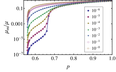
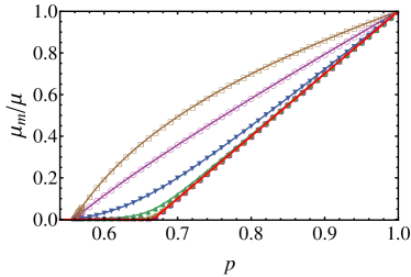
Figure 5: (color online) (a) Semi-log plot for the EMT solution $\mu_{m}/\mu=G/G_{0}$ as a function of $p$ for $\mu=1$ and $\kappa=1,10^{-1},10^{-2},10^{-3},10^{-4},10^{-5},10^{-6}$ from top to bottom, as indicated in the legend. (b) Linear plot of $\mu_{m}/\mu$ as a function of $p$, with parameters and color code the same as in (a). The red solid line indicates $\mu_{m}$ for the case of a central force triangular lattice ($\kappa=0$). Here and in Figs. 6 to 8, we have set $a=1$. The contents of (a) appeared in a different form in Ref. Broedersz et al. (2011).

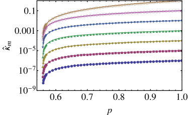
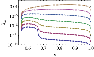
Figure 6: (color online) The EMT solution for $\kappa_{m}$ expressed in terms of the dimensionless combination $\hat{\kappa}_{m}=\kappa_{m}/(\mu a^{2})$ (a) and $\lambda_{m}$ expressed in terms of the dimensionless combination $\hat{\lambda}_{m}=\lambda_{m}/(\mu a^{2})$(b). Parameters and color code are the same as in Fig. 5.

In Figs. 7 and 8 we respectively plot our numerical solutions to the EMT equations near $p_{\textrm{b}}$ and $p_{\textrm{CF}}$ using the analytic scaling forms of Eqs. (47) and (III.1). As required the numerical solutions agree with the analytic ones.

Figure 7: (Color online) Asymptotic solution (dashed lines) and numerical solutions (data points) of $\mu_{m}/\mu=G/G_{0}$ near $p_{\textrm{b}}$. Parameters and color code are the same as in Fig. 5.

Figure 8: (color online) (a), (b), and (c) show rescaled plots of the EMT solutions $\mu_{m}/\mu$, $\kappa_{m}$ and $\lambda_{m}$ using the scaling forms (53a) for $\mu=1$ and $\kappa=10^{-2},10^{-3},10^{-4},10^{-5},10^{-6}$, with color code the same as in Fig. 5, and exponents taking the value as in Eq. (54a). The thin black lines represent the asymptotic forms of Eq. (55a) for small $\kappa$. The brown dash-dotted lines, the thick blue solid lines, and the purple dashed lines plot the functional form of $\mu_{m}$ obtained in the crossover, the stretching-dominated, and the bending-dominated regimes of Eq. (III.1), respectively. The contents of (a) appeared in a different from in Ref. (Broedersz et al. (2011))

V Discussion

Two other approaches, one by Das et al. Das et al. (2007, 2012) and one by Wyart et al. Wyart et al. (2008), produce results similar to ours, and below we briefly review compare them to ours. References Heussinger and Frey (2006) and Heussinger et al. (2007), which develop an EMT for fiber networks like the Mikado model with a maximum coordination number of four, do not consider rigidity development on a triangular lattice with a maximum coordination number of six, and we will not discuss them further.

Stretching forces are easily described by CF springs, which reside on bonds, each of which can have a distinct spring constant. Bending forces, on the other hand, couple angles on neighboring $NN$ bonds, or equivalently $NNN$ sites along a filament to the site between them via phantom $NNN$ bonds. Because removing one $NN$ bond from a pair defining a phantom $NNN$ bending bond effectively removes that phantom bond, bending and stretching are not independent in the diluted lattice. This presents real challenges for the development of a consistent bend-stretch EMT.

Our approach to this problem appeals to the underlying polymer nature of our model in which constituent polymers are endowed with local stretching and bending moduli $\mu$ and $\kappa$. We can modify these moduli along any bond. Different stretch moduli lead to independent effective CF stretch force constants $k_{||}=\mu/a$ for each bond. Modification of the bending modulus $\kappa$ on a given $NN$ bond, however, modifies the bend force constant $k_{\perp}=\kappa/a^{3}$ for both phantom $NNN$ bonds that that $NN$ bond partially defines in the manner described above. With this approach, we develop a consistent EMT that includes the statistical correlation between bend and stretch.

Das et al. begin by ignoring the correlation between real $NN$ bonds and phantom $NNN$ bonds and assume that a stretch spring on a given $NN$ bond can be removed without affecting the bending energy on the phantom $NNN$ bonds that include that $NN$ bond and that bending springs on the phantom $NNN$ bonds can be removed without affecting the stretch springs on the two bonds that define the $NNN$ bond. In other words, the phantom bond is effectively elevated to a real bond with existence independent of the underlying $NN$ bonds. In general, the $NNN$ bonds can be present with with an arbitrary probability $q$ and absent with probability $1-q$. To provide an approximate description of the constraint that the phantom bond does not exist unless both of the $NN$ bonds defining it are present, Das et al. assign a probability $q=p^{2}$ ($p$ is the probability that a $NN$ bond is occupied) to the occupancy of a $NNN$ bending bond, but continue to treat the $NN$ and $NNN$ bonds as statistically independent. Again the result is a set of closed self-consistent equations for $\mu_{m}$ and $\kappa_{m}$, which we analyze in our formulation of EMT in App. C.

Both approaches yield $p_{\textrm{CF}}=2/3$ in good agreement with numerical estimates Wang et al. (1992); Sahimi (1998); Broedersz et al. (2011), which yield $p_{\textrm{CF}}$ of order $0.64$ or $0.65$. Our approach yields a value for $p_{\textrm{b}}$ (0.56) that is well above that (0.445) observed in simulations Broedersz et al. (2011) whereas that of Ref. Das et al. (2012) yields a value ($p_{\textrm{b}}=0.457$) in good agreement with simulations. The latter method produces results in better agreement with simulations over the entire range of values of $p$ than does ours if no approximations to the EMT equations are used in the numerical evaluation of the shear modulus [See App. C]. It is not clear to us why this is so. Both approaches yield a nontrivial bend-stretch crossover, with the same algebraic form but with slightly different parameters [See App. C] in the vicinity of $p_{\textrm{CF}}$ in qualitative agreement with simulations.

In Ref. Wyart et al. (2008), Wyart et al. consider random off-lattice elastic networks derived from two-dimensional packings of spheres O’Hern et al. (2003) with a cordination number above the Maxwell CF isostatic limit of $z=4$ in which CF springs are assigned to each sphere-sphere contact. They use numerical simulations to study the nonlinear relation between shear stress $\sigma$ and shear strain $\gamma$ as springs are cut, thereby reducing $z$, and they find a scaling relation $\sigma=\gamma|\delta z|f(\gamma/|\delta z|)$, where $\delta z=z-4$, $f(x)\to{\rm const.}$ for $x\to 0^{+}$, $f(x)\to 0$ for $x\to 0^{-}$, and $f(x)\sim x$ for $x\to\infty$. This scaling form predicts $\sigma\sim\gamma$ for $\delta z\gg\gamma>0$, $\sigma=0$ for $\delta z\ll-\gamma<0$, and $\sigma\sim\gamma^{2}$ for $\gamma\gg\delta z$. Reference Wyart et al. (2008) then provides a theoretical justification for this behavior based upon the existence of a plateau in the density of states Silbert et al. (2005) above $\omega^{*}\sim\delta z$ and reasonable assumptions about statistical independence of eigenvectors associated with different normal modes in the isostatic network Maloney (2006) and about the nature of nonaffine response of nearly isostatic systems. Finally, they extend this line of reasoning to nearly isostatic systems with extra weak bonds and find three regimes of elastic response that are identical to those we identify in Eqs. (53a) to (55a) if the weak bonds are of a bending type.

To summarize we developed an effective-medium theory that can include bending energy of filaments, and we used it to study the development of rigidity of a randomly diluted triangular lattice with central force springs on occupied bonds and bending forces between occupied bond pairs along a straight line. We obtained a rigidity threshold for positive bending stiffness and a crossover, controlled by the isostatic point of the central force triangular lattice, characterizing bending-dominated, stretching-dominated, and stretch-bend coupled elastic regimes.

Acknowledgments—We are grateful to C. P. Broedersz and F.C. MacKintosh for many stimulating and helpful discussions. This work was supported in part by the National Science Foundations under grants DMR-0804900 and DMR-1104707 and under the Materials Research Science and Engineering Center DMR11-20901 .

Appendix A Discretization of a continuous rod

In this appendix, we will derive the discretized bending energy for an inhomogeneous rod from the continuous bending energy in of Eq. (1). We divide the rod into bonds of length $a$ whose endpoints are at nodes $i$ (which coincide with vertices of our lattice) as shown in Fig. 2. Segment $i$, which lies between nodes $i-1$ and $i$, is endowed with a bending modulus $\kappa_{i}$, and the angle at its center is constrained to be $\theta_{i}$. Within each segment $i$, the angle $\theta_{i}(t)$ with $-a/2<t<a/2$ ]i.e., within segment $i$, $t=s-ia$] minimizes the bending energy in that segment and satisfies the equation $d^{2}\theta_{i}(t)/dt^{2}=0$ subject to the boundary conditions (BCs) for each $i$

$$(1)\,\,\, \theta_{i}(t=0) = \theta_{i},$$

$$(2)\,\,\, \theta_{i+1}(-a/2) = \theta_{i}(a/2),$$

$$(3)\,\,\, \kappa_{i}\left.\frac{d\theta_{i}}{ds}\right|_{t=a/2} = \kappa_{i+1}\left.\frac{d\theta_{i+1}}{ds}\right|_{ts=-a/2}.$$ (63)

BC (1) is the constraint that $\theta(t)$ take on the value $\theta_{i}$ at the center of bond $i$; BC(2) is the condition that $\theta(t)$ be continuous at node $i$; and BC(3) is the condition that the torque on node $i$ be zero. Thus, within segment $i$,

$$\theta_{i}(t)=\begin{cases}\theta_{i}+A_{i}^{-}s&\mbox{if }-a/2<t<0\\ \theta_{i}+A_{i}^{+}s&\mbox{if }\,\,0<t<a/2.\end{cases}$$ (64)

This form immediately satisfies boundary condition $(1)$. Boundary condition $(2)$ requires

$$\theta_{i}+\frac{a}{2}A_{i}^{+}=\theta_{i+1}-\frac{a}{2}A_{i+1}^{-},$$ (65)

and boundary condition $(3)$ requries

$$\kappa_{i}A_{i}^{+}=\kappa_{i+1}A_{i+1}^{-}.$$ (66)

The solution of Eq. (65) and (66) for $A_{i}^{+}$ and $A_{i+1}^{-}$ is

$$A_{i}^{+}=\frac{2}{a}\frac{\kappa_{i+1}}{\kappa_{i}+\kappa_{i+1}}(\theta_{i+1}-\theta_{i})=\frac{\kappa_{i+1}}{\kappa_{i}}A_{i+1}^{-}.$$ (67)

With this result, we can calculate the bending energy of the segment running from the midpoint of bond $i$ to the midpoint of bond $i+1$:

$$E_{i} =\frac{1}{2}\kappa_{i}\int_{0}^{a/2}\left(\frac{d\theta_{i}}{ds}\right)^{2}+\frac{1}{2}\kappa_{i+1}\int_{-a/2}^{0}\left(\frac{d\theta_{i+1}}{ds}\right)^{2}$$

$$=\frac{1}{2}\frac{a}{2}\left[\kappa_{i}(A_{i}^{+})^{2}+\kappa_{i+1}(A_{i+1}^{-})^{2}\right]$$

$$=\frac{1}{2a}\kappa_{i}^{\text{eff}}(\Delta\theta_{i})^{2},$$ (68)

where $\Delta\theta_{i}=\theta_{i+1}-\theta_{i}$ and

$$\overline{\kappa}_{i}=\frac{2\kappa_{i+1}\kappa_{i}}{\kappa_{i+1}+\kappa_{i}}.$$ (69)

When $\kappa_{i}=\kappa_{i+1}$, this reduces to $\kappa_{i}$. The total energy, apart from boundary terms, which we ignore, is then $E=\sum_{i}E_{i}$. When all $\kappa_{i}$ are equal, this is indeed exactly the discretized form that we use. If the bending modulus $\kappa_{i}$ on segment (bond) $i$ differs from the modulus $\kappa$ on all of the other bonds, then the bending energies associated with site $i-1$ and $i$ will have an “effective” modulus $2\kappa_{i}\kappa/(\kappa_{i}+\kappa)$ in agreement with our EMT treatment.

It is instructive to verify that the continuum and the discretized theory give the same result for a particular inhomogeneous $\kappa$. For simplicity, we consider a filament of length $L$ whose left and right ends coincide with bond centers (rather than nodes) at positions $t=0$ and $t=L$, respectively. There are thus $N-1$ contiguous bonds of length $a$ terminated by two half bonds of length $a/2$. We assume that the bending modulus is equal to $\kappa_{1}$ in regions I defined by $0\leq t<t_{p}=[p-(1/2)]a$ and to $\kappa_{2}$ in regions II defined by $t_{p}<s<\leq L$, and we assign boundary conditions that $\theta(0)=0$ and $\theta(L)=\Theta$. Consider first the continuum case. $d^{2}\theta(t)/dt^{2}=0$ in both regions I and II, and as a result the solutions for $\theta$ in these two regions that satisfy the boundary conditions are, respectively, $\theta_{1}=B_{1}(t/a)$ and $\theta_{2}=\Theta+B_{2}[(t-L)/a]$. The additional boundary conditions are that $\theta$ and $\kappa d\theta/dt$ be continuous at $t=t_{p}$, implying

$$(B_{1}/a)t_{p} = \Theta+(B_{2}/a)(t_{p}-L),$$

$$\kappa_{1}B_{1}/a = \kappa_{2}B_{2}/a.$$ (70)

These equations are easily solved for $B_{1}$ and $B_{2}$:

$$\kappa_{1}=\frac{\kappa_{2}\Theta}{(\kappa_{2}-\kappa_{1})(t/a)+\kappa_{1}(L/a)}=\frac{\kappa_{2}}{\kappa_{1}}B_{2}.$$ (71)

In the discrete case, nodes $i=1$ to $p-1$ have bending energy $(1/2)\kappa_{1}(\theta_{i+1}-\theta_{i})^{2}$, nodes $i=p+1$ to $(N-1)$ have bending energy $(1/2)\kappa_{2}(\theta_{i+1}-\theta_{i})^{2}$, and site $p$ has bending energy $(1/2)\overline{\kappa}(\theta_{p+1}-\theta_{p})^{2}$. The equations for $\theta_{i}$, $i=1,\cdots N-1$ are thus,

$$\frac{dE}{d\theta_{i}} =\kappa_{b}(2\theta_{i}-\theta_{i+1}-\theta_{i-1})=0;\,\,\,\,1<i<p-1$$

$$\frac{dE}{d\theta_{p-1}} =\kappa_{b}(\theta_{p-1}-\theta_{p-2})+\overline{\kappa}(\theta_{p-1}-\theta_{p})=0;$$

$$\frac{dE}{d\theta_{p}} =\overline{\kappa}(\theta_{p}-\theta_{p-1})+\kappa_{a}(\theta_{p}-\theta_{p+1})=0;$$

$$\frac{dE}{d\theta_{i}} =\kappa_{a}(2\theta_{i}-\theta_{i+1}-\theta_{i-1})=0;\,\,\,\,p<i\leq N-2.$$ (72)

These linear difference equations subject to the boundary conditions, $\theta_{0}=0$ and $\theta_{N}=\Theta$ are solved by setting $\theta_{i}=D_{1}i$ in region I ($0\leq i\leq p$) and $\theta_{i}=\Theta+D_{2}(i-N)$ in region II ($p<i\leq N$). The equilibrium equations for $\theta_{p}$ and $\theta_{p-1}$ are

$$[\kappa_{1}+\overline{\kappa}(p-1)]D_{1}-\overline{\kappa}(p-n)D_{2} = \,\,\overline{\kappa}\,\Theta,$$

$$-\overline{\kappa}(p-1)D_{1}+[\overline{\kappa}(p-N)-\kappa_{2}]D_{2} = -\overline{\kappa}\,\Theta.$$ (73)

These equations, along with the relation $\overline{\kappa}=2\kappa_{1}\kappa_{2}/(\kappa_{1}+\kappa_{2})$, yield $D_{1}=B_{1}$ and $D_{2}=B_{2}$ verifying that the discrete and continuum solutions agree.

Finally, we need to specify the relation between angles $\theta_{i}$ and the vertical displacements $h_{i}$ (i.e., $u_{i}^{\perp}$). Let $h^{\prime}_{i}$ be the height at the center of bond $i$. To linear order in continuum theory, $dh(t)/ds=\theta(t)$. Integration of this equation [using Eq. (64)] then yields

$$h_{i}-h^{\prime}_{i} = \int_{0}^{a/2}\theta_{i}(t)dt=(a/2)\theta_{i}+\frac{a^{2}}{8}A_{i}^{+}$$

$$h_{i}^{\prime}-h_{i-1} = \int_{-a/2}^{0}\theta_{i}(t)dt=(a/2)\theta_{i}+\frac{a^{2}}{8}A_{i}^{-}$$ (74)

with the same convention as that of Eqs. (63) and (64). From Eq.(67), $A_{i}^{+}\propto(\theta_{i+1}-\theta_{i})/a$ and $A_{i}^{-}\propto(\theta_{i}-\theta_{i-1})/a$. Thus for slowly varying $\theta$ and small $a$, $a^{2}A_{i}^{+}$ and $a^{2}A_{i}^{-}$ can be ignored relative to $a\theta_{i}$. This is true whether or not $\kappa$ changes from bond to bond. The result is that the slope of $h(s)$ within bond $i$ is simply $\theta_{i}$, and

$$\frac{h_{i}-h_{i-1}}{a}\approx\theta_{i}+\frac{1}{8}a(A_{i}^{+}-A_{i}^{-}).$$ (75)

Appendix B The dynamical matrix and the phonon Green’s function of the effective medium

From Eq. (III), it is straightforward to calculate the components of the dynamical matrix of the effective medium:

$$\mathbf{D}^{(m)}=\left(\begin{array}[]{cc}D_{xx}&D_{xy}\\ D_{yx}&D_{yy}\end{array}\right),$$ (78)

where

$$D_{xx}= \mu_{m}\left[3-2\cos q_{x}-\cos(q_{x}/2)\cos(\sqrt{3}q_{y}/2)\right]+3\kappa_{m}\left[3-4\cos(q_{x}/2)\cos(\sqrt{3}q_{y}/2)+\cos(q_{x})\cos(\sqrt{3}q_{y})\right]$$

$$+3\lambda_{m}\left[-4+7\cos(q_{x}/2)\cos(\sqrt{3}q_{y}/2)-4\cos(q_{x})\cos(\sqrt{3}q_{y})+\cos(3q_{x}/2)\cos(3\sqrt{3}q_{y}/2)\right]$$

$$D_{xy}= \sqrt{3}(\mu_{m}-4\kappa_{m}+7\lambda_{m})\sin(q_{x}/2)\sin(\sqrt{3}q_{y}/2)+\sqrt{3}(\mu_{m}-4\lambda_{m})\sin q_{x}\sin(\sqrt{3}q_{y})$$

$$+\sqrt{3}\lambda_{m}\sin(3q_{x}/2)\sin(3\sqrt{3}q_{y}/2)$$

$$D_{yx}= D_{xy}$$

$$D_{yy}= 3\mu_{m}\left[1-\cos(q_{x}/2)\cos(\sqrt{3}q_{y}/2)\right]$$

$$+\kappa_{m}\left[9-8\cos q_{x}+2\cos(2q_{x})-4\cos(q_{x}/2)\cos(\sqrt{3}q_{y}/2)+\cos(q_{x})\cos(\sqrt{3}q_{y})\right]$$

$$+\lambda_{m}\Big{[}-12+14\cos q_{x}-8\cos(2q_{x})+2\cos(3q_{x})+7\cos(q_{x}/2)\cos(\sqrt{3}q_{y}/2)$$

$$\quad\quad-4\cos(q_{x})\cos(\sqrt{3}q_{y})+\cos(3q_{x}/2)\cos(3\sqrt{3}q_{y}/2)\Big{]}.$$ (79)

The symmetry properties of the above components of $\mathbf{D}^{(m)}$ will determine which components of $\tilde{G}^{(m)}$ are nonzero. $D_{11}(q_{x},q_{y})$ and $D_{22}(q_{x},q_{y})$ are even under $q_{x}\rightarrow-q_{x}$ and under $q_{y}\rightarrow-q_{y}$ whereas $D_{12}(q_{x},q_{y})$ is odd under the same operations.

The effective medium phonon Green’s function is the negative of the inverse of $\mathbf{D}^{(m)}$

$$\mathbf{G}^{(m)}= -(\mathbf{D}^{(m)})^{-1}$$

$$= (\textrm{Det}\mathbf{D}^{(m)})^{-1}\left(\begin{array}[]{cc}D_{yy}&-D_{xy}\\ -D_{yx}&D_{yy}\end{array}\right).$$ (82)

The determinant $\textrm{Det}\mathbf{D}^{(m)}=D_{xx}D_{yy}-D_{xy}D_{yx}$ is even under $q_{x}\rightarrow-q_{x}$ and under $q_{y}\rightarrow-q_{y}$, and thus $xx$ and $yy$ components of $\mathbf{G}^{(m)}$ are both even and the $xy$ component of $\mathbf{G}^{(m)}$ is odd under $q_{x}\rightarrow-q_{x}$ and under $q_{y}\rightarrow-q_{y}$. With this information and the properties of $\mathbf{B}^{s}_{n,\mathbf{q}}$ and $\mathbf{B}^{b}_{n,\mathbf{q}}$, we can infer which components of $\tilde{G}^{(m)}$ are zero and which are equal to each other. First consider the $12$ and $13$ components, which from Eq. (36) are given by

$$(\tilde{G}^{(m)})^{12} = \frac{1}{N}\sum_{\mathbf{q}}\mathbf{B}^{s}_{1,-\mathbf{q}}\mathbf{G}^{(m)}_{\mathbf{q}}\mathbf{B}^{b}_{1,\mathbf{q}}$$ (83)

$$(\tilde{G}^{(m)})^{13} = \frac{1}{N}\sum_{\mathbf{q}}\mathbf{B}^{s}_{1,-\mathbf{q}}\mathbf{G}^{(m)}_{\mathbf{q}}\mathbf{B}^{b}_{4,\mathbf{q}}.$$ (84)

$\mathbf{B}^{s}_{1,-\mathbf{q}}$ is a vector parallel to the $x$-axis (i.e., to $\mathbf{e}_{1}$), whereas both $\mathbf{B}^{b}_{1,\mathbf{q}}$ and $\mathbf{B}^{b}_{4,\mathbf{q}}$ are parallel to the $y$-axis (i.e. to $\mathbf{e}^{\perp}_{1}$). In addition, $\mathbf{B}^{s}_{1,-\mathbf{q}}$, $\mathbf{B}^{b}_{1,\mathbf{q}}$, and $\mathbf{B}^{b}_{4,\mathbf{q}}$ are all even under $q_{y}\rightarrow-q_{y}$. Thus the integrands in Eq. (36) are equal to $G_{xy}$ times a function even under $q_{y}\rightarrow-q_{y}$. Since $G_{xy}$ is odd under this operation, both integrals vanish, and the $12$ and $13$ components of $\tilde{G}^{(m)}$ vanish by symmetry. There are no symmetry operations that make the other components of $\tilde{G}^{(m)}$ vanish, but the relation $\mathbf{B}^{b}_{1,-\mathbf{q}}\mathbf{B}^{b}_{1,\mathbf{q}}=\mathbf{B}^{b}_{4,-\mathbf{q}}\mathbf{B}^{b}_{4,\mathbf{q}}$ sets the the $22$ and $33$ component of $\tilde{G}^{(m)}$ equal to each other and leads to Eq. (42) for $\tilde{G}^{(m)}$.

Appendix C Comparison with EMT results obtained using methods in Ref. Das et al. (2007, 2012)

In this section we derive the Das’ EMT equations from our approach (by changing some assumption as detailed below) and calculate it for the triangular lattice. We also compare it to both our EMT and simulation results.

We start from the same effective medium dynamical matrix $\mathbf{D}^{(m)}$ as we defined in the main text ($\mathbf{D}^{(m)}$ with $\mu_{m},\kappa_{m}$ but $\lambda_{m}=0$), but we make different assumptions about the changed bond in the EMT. In particular, the perturbative potential is now

$$E_{V,\textrm{Das}} = \frac{1}{2}\frac{\mu_{s}-\mu_{m}}{a}(\mathbf{u}_{\ell_{1}\ell_{2}}\cdot\hat{\mathbf{r}}_{\ell_{1}\ell_{2}})^{2}$$ (85)

$$+\frac{1}{2}\frac{\kappa_{s}-\kappa_{m}}{a^{3}}\theta_{\ell_{1}\ell_{2}\ell_{3}}^{2},$$

and the differences comparing with our version are: (i) there is only 1 bending energy term $\theta_{\ell_{1}\ell_{2}\ell_{3}}^{2}$ and the other term $\theta_{\ell_{0}\ell_{1}\ell_{2}}^{2}$ is not included, (ii) the bending stiffness is directly $\kappa_{s}$ instead of our composite one $\kappa_{c}(\kappa_{s})$, and (iii) there is no $\lambda_{m}$ term.

The matrix form of $V$ in the space of $\{\mathbf{B}_{1}^{s},\mathbf{B}_{1}^{b}\}$ is then (now $\mathbf{B}_{4}^{b}$ is not relevant)

$$\tilde{\mathbf{V}}_{\textrm{Das}}=\left(\begin{array}[]{cc}(\mu_{s}-\mu_{m})/a&0\\ 0&(\kappa_{s}-\kappa_{m})/a^{3}\end{array}\right)$$ (88)

Thus it is clear that

$$\tilde{\mathbf{T}}_{\textrm{Das}}=(\tilde{\mathbf{V}}_{\textrm{Das}}^{-1}-\tilde{\mathbf{G}}^{(m)})^{-1}$$ (89)

is also a diagonal matrix (we have already proved in the text that $\tilde{\mathbf{G}}^{(m)}$ is diagonal due to symmetry).

Correspondingly the probability distribution is now

$$P_{\textrm{Das}}(\mu_{s},\kappa_{s})= \Big{[}p\delta(\mu_{s}-\mu)+(1-p)\delta(\mu_{s})\Big{]}$$

$$\times\Big{[}p^{2}\delta(\kappa_{s}-\kappa)+(1-p^{2})\delta(\kappa_{s})\Big{]},$$ (90)

with the distribution of $\mu_{s}$ and $\kappa_{s}$ factorized.

Therefore the EMT matrix equation

$$\int d\mu_{s}d\kappa_{s}P_{\textrm{Das}}(\mu_{s},\kappa_{s})\tilde{\mathbf{T}}_{\textrm{Das}}(\mu_{s},\kappa_{s})=0$$ (91)

decouples to two equations of the two diagonal elements (they still share the same variables) that

$$\frac{\mu_{m}}{\mu} =\frac{p-a^{*}}{1-a^{*}}$$

$$\frac{\kappa_{m}}{\kappa} =\frac{p^{2}-b^{*}}{1-b^{*}}$$ (92)

where

$$a^{*} =\frac{\mu_{m}}{a}\frac{1}{N}\sum_{\mathbf{q}}\mathbf{B}_{1,-\mathbf{q}}^{s}\cdot\mathbf{D}^{(m)}_{\mathbf{q}}\cdot\mathbf{B}_{1,\mathbf{q}}^{s}$$

$$b^{*} =\frac{\kappa_{m}}{a}\frac{1}{N}\sum_{\mathbf{q}}\mathbf{B}_{1,-\mathbf{q}}^{b}\cdot\mathbf{D}^{(m)}_{\mathbf{q}}\cdot\mathbf{B}_{1,\mathbf{q}}^{b}.$$ (93)

which is exactly the equations from Mo’s paper.

In contrast the distribution in our EMT is

$$P(\mu_{s},\kappa_{s})=p\delta(\mu_{s}-\mu)\delta(\kappa_{s}-\kappa)+(1-p)\delta(\mu_{s})\delta(\kappa_{s})$$ (94)

with the distribution of $\mu_{s}$ and $\kappa_{s}$ correlated. This is more reasonable because they describe the same replaced bond. Furthermore, $\kappa_{s}$ affects two bending terms.

To summarize, the stretching bonds and “bending bonds”are treated as independent in the Das’ EMT, whereas we model them as describing filament properties and thus correlated.

From the definition of $\mathbf{D}^{(m)}$ it is clear that

$$a^{*}+b^{*} =\frac{2}{z}\,\textrm{tr}\Big{\{}\frac{1}{N}\sum_{\mathbf{q}}\big{[}\mathbf{D}^{(m)}_{\mathbf{q}}\big{]}^{-1}\mathbf{D}^{(m)}_{\mathbf{q}}\Big{\}}$$

$$=\frac{2d}{z}=2/3$$ (95)

The self-consistency equation (C) can be solved numerically for any given $p$, $\mu$, and $\kappa$. In particular, the rigidity threshold $p_{\textrm{b}}$ can be solved analytically from

$$0 =p-a^{*}$$

$$0 =p^{2}-b^{*}$$ (96)

which leads to

$$p_{\textrm{b}}=\frac{1}{2}\left(-1+\sqrt{1+\frac{8d}{z}}\right)$$ (97)

and for the triangular lattice it gives

$$p_{\textrm{b}}\simeq 0.4574.$$ (98)

The EMT self-consistency equation (C) can be solved numerically, and we plot the results along with ours and the simulation data from Ref. Broedersz et al. (2011) in Fig. 9. The curves calculated from Eq. (C) differ in detail from those presented in Ref. Das et al. (2012) because the latter reference used approximate forms for $a^{*}$ and $b^{*}$ in its numerical evaluations Das and Schwartz

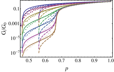
Figure 9: Comparison between the shear modulus (normalized by the shear modulus at $p=1$, so it is equivalent to $\mu_{m}/\mu$) obtained from numerical simulations from Ref. Broedersz et al. (2011)(data points), Das’ EMT (solid lines), and our EMT (dashed lines). Different colors mark different values of $\kappa$ with the same color code as in Fig. 5, and from top to bottom the corresponding values of $\kappa$ are $1$, $10^{-1},10^{-2},\cdots,10^{-6}$.

Near $p_{\textrm{CF}}$ we can also expand the Das’ EMT solution to get the asymptotic behaviors. The functions $a^{*}$ and $b^{*}$ are related to the integrals we defined via

$$a^{*} =H_{1}(b_{m},0)$$

$$b^{*} =b_{m}H_{2}\left(b_{m},0\right).$$ (99)

At $\kappa=0$, because

$$H_{1}(0,0)=p_{\textrm{CF}},\quad H_{2}(0,0)=0$$ (100)

it is straightforward to see that the Das’ EMT lead to the same central force solution as our EMT

$$\mu_{m} =\mu(p-p_{\textrm{CF}})\tilde{\Theta}(p-p_{\textrm{CF}}),$$

$$\kappa_{m} =0,$$ (101)

where $\tilde{\Theta}$ is the Heaviside step function. For small $\kappa>0$ we expand around small $b_{m}=\kappa_{m}/(\mu_{m}a^{2})$. We have already discussed the expansion of $H_{1}$ and $H_{2}$ at this limit, and thus

$$a^{*} =p_{\textrm{CF}}+H_{1,1}b_{m},$$

$$b^{*} =H_{1,1}b_{m}.$$ (102)

Because $H_{1,1}$ is of order unity, $b^{*}\sim b_{m}$ is very small. Therefore we can ignore the $b^{*}$ terms in the equation of $\kappa_{m}$ and get

$$\kappa_{m}\simeq\kappa p^{2},$$ (103)

which differs from our EMT solution

$$\kappa_{m}\simeq\kappa(2p-1)$$ (104)

by the dependence on $p$, but this difference is small and does not show singularity near $p_{\textrm{CF}}$. We can then plug this solution back into the equation for $\mu_{m}$, which turns into a quadratic equation similar to the equation for $\mu_{m}$ in our EMT, with the only difference being the different $p$ dependence of $\kappa_{m}$. We thus arrive at

$$\mu_{m}=\mu|\Delta p|\frac{3}{2}\left(\pm 1+\sqrt{1-\frac{16\mathcal{A}}{27}\frac{\kappa}{a^{2}\mu|\Delta p|^{2}}}\right)$$ (105)

which takes a very similar form to Eq. (III.1) just with a different constant factor before $\kappa/(a^{2}\mu|\Delta p|^{2})$. Therefore the two EMTs produce the same scaling behavior near $p_{\textrm{CF}}$.

References

- Liu and Nagel (1998) \BibitemOpen\bibfieldauthor A. J. Liu and S. R. Nagel, \bibfieldjournal Nature 396, 21 (1998)\BibitemShutNoStop
- Wyart (2005) \BibitemOpen\bibfieldauthor M. Wyart, \bibfieldjournal Ann. Phys. Fr 30, 1 (2005)\BibitemShutNoStop
- Liu and Nagel (2010) \BibitemOpen\bibfieldauthor A. J. Liu and S. R. Nagel, in Annual Review of Condensed Matter Physics, Vol. 1 (2010) pp. 347–369\BibitemShutNoStop
- Phillips (1981) \BibitemOpen\bibfieldauthor J. C. Phillips, \bibfieldjournal J. Non-Cryst. Solids 43, 37 (1981)\BibitemShutNoStop
- Thorpe (1983) \BibitemOpen\bibfieldauthor M. Thorpe, \bibfieldjournal J. Non-Cryst. Solids 57, 355 (1983)\BibitemShutNoStop
- Phillips and Thorpe (1985) \BibitemOpen\bibfieldauthor J. C. Phillips and M. F. Thorpe, \bibfieldjournal Solid State Commun. 53, 699 (1985)\BibitemShutNoStop
- He and Thorpe (1985) \BibitemOpen\bibfieldauthor H. He and M. F. Thorpe, \bibfieldjournal Phys. Rev. Lett. 54, 2107 (1985)\BibitemShutNoStop
- Thorpe et al. (2000) \BibitemOpen\bibfieldauthor M. Thorpe, D. Jacobs, M. Chubynsky, and J. Phillips, \bibfieldjournal J. Non-Cryst. Solids 266, 859 (2000)\BibitemShutNoStop
- Elson (1988) \BibitemOpen\bibfieldauthor E. Elson, \bibfieldjournal Annu. Rev. Biophys. Chem. 17, 397 (1988)\BibitemShutNoStop
- Kasza et al. (2007) \BibitemOpen\bibfieldauthor K. Kasza, A. Rowat, J. Liu, T. Angelini, C. Brangwynne, G. Koenderink, and D. Weitz, \bibfieldjournal Curr. Opinion Cell Biology 19, 101 (2007)\BibitemShutNoStop
- Alberts et al. (2008) \BibitemOpen\bibfieldauthor B. Alberts, A. Johnson, J. Lewis, M. Raff, K. Roberts, and P. Walter, Molecular Biology of the Cell, 4th ed. (Garland, New York, 2008)\BibitemShutNoStop
- Janmey et al. (1997) \BibitemOpen\bibfieldauthor P. Janmey, S. Hvidt, J. Lamb, and T. Stossel, \bibfieldjournal Nature 345, 89 (1997)\BibitemShutNoStop
- MacKintosh et al. (1995) \BibitemOpen\bibfieldauthor F. C. MacKintosh, J. Käs, and P. A. Janmey, \bibfieldjournal Phys. Rev. Lett. 75, 4425 (1995)\BibitemShutNoStop
- Head et al. (2003) \BibitemOpen\bibfieldauthor D. A. Head, A. J. Levine, and F. C. MacKintosh, \bibfieldjournal Phys. Rev. Lett. 91, 108102 (2003)\BibitemShutNoStop
- Wilhelm and Frey (2003) \BibitemOpen\bibfieldauthor J. Wilhelm and E. Frey, \bibfieldjournal Phys. Rev. Lett. 91, 108103 (2003)\BibitemShutNoStop
- Head et al. (2005) \BibitemOpen\bibfieldauthor D. A. Head, A. J. Levine, and F. C. MacKintosh, \bibfieldjournal Phys. Rev. E 72, 061914 (2005)\BibitemShutNoStop
- Storm et al. (2005) \BibitemOpen\bibfieldauthor C. Storm, J. Pastore, F. MacKintosh, T. Lubensky, and P. Janmey, \bibfieldjournal Nature 435, 191 (2005)\BibitemShutNoStop
- Onck et al. (2005) \BibitemOpen\bibfieldauthor P. R. Onck, T. Koeman, T. van Dillen, and E. van der Giessen, \bibfieldjournal Phys. Rev. Lett. 95, 178102 (2005)\BibitemShutNoStop
- Huisman et al. (2007) \BibitemOpen\bibfieldauthor E. M. Huisman, T. van Dillen, P. R. Onck, and E. Van der Giessen, \bibfieldjournal Phys. Rev. Lett. 99, 208103 (2007)\BibitemShutNoStop
- Huisman and Lubensky (2010) \BibitemOpen\bibfieldauthor E. M. Huisman and T. C. Lubensky, \bibfieldjournal Phys. Rev.Lett 106, 088301 (2011)\BibitemShutNoStop
- Feng and Sen (1984) \BibitemOpen\bibfieldauthor S. Feng and P. N. Sen, \bibfieldjournal Phys. Rev. Lett. 52, 216 (1984)\BibitemShutNoStop
- Feng et al. (1984) \BibitemOpen\bibfieldauthor S. Feng, P. N. Sen, B. I. Halperin, and C. J. Lobb, \bibfieldjournal Phys. Rev. B 30, 5386 (1984)\BibitemShutNoStop
- Jacobs and Thorpe (1995) \BibitemOpen\bibfieldauthor D. J. Jacobs and M. F. Thorpe, \bibfieldjournal Phys. Rev. Lett. 75, 4051 (1995)\BibitemShutNoStop
- Maxwell (1864) \BibitemOpen\bibfieldauthor J. C. Maxwell, \bibfieldjournal Philos. Mag. 27, 294 (1864)\BibitemShutNoStop
- Calladine (1978) \BibitemOpen\bibfieldauthor C. Calladine, \bibfieldjournal Int. J. Solids Struct. 14, 161 (1978)\BibitemShutNoStop
- Jacobs and Thorpe (1996) \BibitemOpen\bibfieldauthor D. J. Jacobs and M. F. Thorpe, \bibfieldjournal Phys. Rev. E 53, 3682 (1996)\BibitemShutNoStop
- Soven (1969) \BibitemOpen\bibfieldauthor P. Soven, \bibfieldjournal Phys. Rev. 178, 1136 (1969)\BibitemShutNoStop
- Elliott et al. (1974) \BibitemOpen\bibfieldauthor R. J. Elliott, J. A. Krumhansl, and P. L. Leath, \bibfieldjournal Rev. Mod. Phys. 46, 465 (1974)\BibitemShutNoStop
- Feng et al. (1985) \BibitemOpen\bibfieldauthor S. Feng, M. F. Thorpe, and E. Garboczi, \bibfieldjournal Phys. Rev. B 31, 276 (1985)\BibitemShutNoStop
- Garboczi and Thorpe (1985) \BibitemOpen\bibfieldauthor E. J. Garboczi and M. F. Thorpe, \bibfieldjournal Phys. Rev. B 31, 7276 (1985)\BibitemShutNoStop
- Schwartz et al. (1985) \BibitemOpen\bibfieldauthor L. M. Schwartz, S. Feng, M. F. Thorpe, and P. N. Sen, \bibfieldjournal Phys. Rev. B 32, 4607 (1985)\BibitemShutNoStop
- Das et al. (2007) \BibitemOpen\bibfieldauthor M. Das, F. C. MacKintosh, and A. J. Levine, \bibfieldjournal Phys. Rev. Lett. 99, 038101 (2007)\BibitemShutNoStop
- Heussinger and Frey (2006) \BibitemOpen\bibfieldauthor C. Heussinger and E. Frey, \bibfieldjournal Phys. Rev. Lett. 97, 105501 (2006)\BibitemShutNoStop
- Heussinger et al. (2007) \BibitemOpen\bibfieldauthor C. Heussinger, B. Schaefer, and E. Frey, \bibfieldjournal Phys. Rev. E 76, 031906 (2007)\BibitemShutNoStop
- Broedersz et al. (2011) \BibitemOpen\bibfieldauthor C. P. Broedersz, X. M. Mao, T. C. Lubensky, and F. C. MacKintosh, \bibfieldjournal Nature Physics 7, 983 (2011)\BibitemShutNoStop
- Das et al. (2012) \BibitemOpen\bibfieldauthor M. Das, D. A. Quint, and J. M. Schwarz, \bibfieldjournal PLoS One 7, e35939 (2012)\BibitemShutNoStop
- Wyart et al. (2008) \BibitemOpen\bibfieldauthor M. Wyart, H. Liang, A. Kabla, and L. Mahadevan, \bibfieldjournal Phys. Rev. Lett. 101, 215501 (2008)\BibitemShutNoStop
- Sahimi (1998) \BibitemOpen\bibfieldauthor M. Sahimi, \bibfieldjournal Physics Reports-Review Section of Physics Letters 306, 214 (1998)\BibitemShutNoStop
- Wang et al. (1992) \BibitemOpen\bibfieldauthor J. Wang, A. B. Harris, and J. Adler, \bibfieldjournal Phys. Rev. B 45, 7084 (1992)\BibitemShutNoStop
- Straley (1976) \BibitemOpen\bibfieldauthor J. P. Straley, \bibfieldjournal J. of Phys. C Solid State 9, 783 (1976)\BibitemShutNoStop
- Latva-Kokko and Timonen (2001) \BibitemOpen\bibfieldauthor M. Latva-Kokko and J. Timonen, \bibfieldjournal Phys. Rev. E 64, 066117 (2001)\BibitemShutNoStop
- Mao et al. (2011) \BibitemOpen\bibfieldauthor X. Mao, O. Stenull, and T. C. Lubensky, \bibfieldjournal Unpublished (2011)\BibitemShutNoStop
- Stenull and Lubensky (2011) \BibitemOpen\bibfieldauthor O. Stenull and T. C. Lubensky, \bibfieldjournal arXiv:1108.4328v1 [cond-mat.soft] (2011)\BibitemShutNoStop
- Alexander (1998) \BibitemOpen\bibfieldauthor S. Alexander, \bibfieldjournal Phys. Rep. 296, 65 (1998)\BibitemShutNoStop
- Boolchand et al. (2005) \BibitemOpen\bibfieldauthor P. Boolchand, G. Lucovsky, J. C. Phillips, and M. F. Thorpe, \bibfieldjournal Philos. Mag. 85, 3823 (2005)\BibitemShutNoStop
- Marko and Siggia (1995) \BibitemOpen\bibfieldauthor J. Marko and E. Siggia, \bibfieldjournal Macromolecules 28, 8759 (1995)\BibitemShutNoStop
- Kirkpatrick et al. (1970) \BibitemOpen\bibfieldauthor S. Kirkpatrick, B. Velický, and H. Ehrenreich, \bibfieldjournal Phys. Rev. B 1, 3250 (1970)\BibitemShutNoStop
- Mao et al. (2010) \BibitemOpen\bibfieldauthor X. Mao, N. Xu, and T. C. Lubensky, \bibfieldjournal Phys. Rev. Lett. 104, 085504 (2010)\BibitemShutNoStop
- Arbabi and Sahimi (1993) \BibitemOpen\bibfieldauthor S. Arbabi and M. Sahimi, \bibfieldjournal Phys. Rev. B 47, 695 (1993)\BibitemShutNoStop
- O’Hern et al. (2003) \BibitemOpen\bibfieldauthor C. S. O’Hern, L. E. Silbert, A. J. Liu, and S. R. Nagel, \bibfieldjournal Phys. Rev. E 68, 011306 (2003)\BibitemShutNoStop
- Silbert et al. (2005) \BibitemOpen\bibfieldauthor L. E. Silbert, A. J. Liu, and S. R. Nagel, \bibfieldjournal Phys. Rev. Lett. 95, 098301 (2005)\BibitemShutNoStop
- Maloney (2006) \BibitemOpen\bibfieldauthor C. E. Maloney, \bibfieldjournal Phys. Rev. Lett. 97, 035503 (2006)\BibitemShutNoStop
- (53) \BibitemOpen\bibfieldauthor M. Das and J. Schwartz, Private Communication \BibitemShutNoStop