The spatial structure of mono-abundance sub-populations of the Milky Way disk

Abstract

The spatial, kinematic, and elemental-abundance structure of the Milky Way’s stellar disk is complex, and has been difficult to dissect with local spectroscopic or global photometric data. Here, we develop and apply a rigorous density modeling approach for Galactic spectroscopic surveys that enables investigation of the global spatial structure of stellar sub-populations in narrow bins of $[\alpha\mathrm{/Fe}]$ and $[\mathrm{Fe/H}]$, using 23,767 G-type dwarfs from SDSS/SEGUE, which effectively sample $5<R_{GC}<12$ kpc and 0.3 $\lesssim|Z|\lesssim 3$ kpc. We fit models for the number density of each such ([$\alpha$/Fe] & [Fe/H]) mono-abundance component, properly accounting for the complex spectroscopic SEGUE sampling of the underlying stellar population, as well as for the metallicity and color distributions of the samples. We find that each mono-abundance sub-population has a simple spatial structure that can be described by a single exponential in both the vertical and radial direction, with continuously increasing scale heights ($\approx$200 pc to 1 kpc) and decreasing scale lengths ($>$4.5 kpc to 2 kpc) for increasingly older sub-populations, as indicated by their lower metallicities and $[\alpha\mathrm{/Fe}]$ enhancements. That the abundance-selected sub-components with the largest scale heights have the shortest scale lengths is in sharp contrast with purely geometric ‘thick–thin disk’ decompositions. To the extent that [$\alpha$/Fe] is an adequate proxy for age, our results directly show that older disk sub-populations are more centrally concentrated, which implies inside-out formation of galactic disks. The fact that the largest scale-height sub-components are most centrally concentrated in the Milky Way is an almost inevitable consequence of explaining the vertical structure of the disk through internal evolution. Whether the simple spatial structure of the mono-abundance sub-components, and the striking correlations between age, scale length, and scale height can be plausibly explained by satellite accretion or other external heating remains to be seen.

1. Introduction

The formation of galactic disks is a long-standing problem in galaxy formation. In numerical simulations, disks form through gas dissipation (Sandage et al., 1970; Larson, 1976), and the formation of the outer regions of the disk happens on longer time scales than the inner disk (Gott & Thuan, 1976; Larson, 1976; Katz & Gunn, 1991). The disks that form have exponential density profiles (Lake & Carlberg, 1988), possibly due to the detailed conservation of angular momentum of an initially spherical cloud in solid-body rotation (Fall & Efstathiou, 1980; Gunn, 1982). Yet, direct observational evidence for this picture is scant (e.g., Dalcanton et al., 1997; Somerville et al., 2008; Wang et al., 2011), and forming realistic disks within the $\Lambda$CDM paradigm remains challenging (e.g., Abadi et al., 2003; Scannapieco et al., 2009; Guedes et al., 2011).

Central to the question as to how galactic disks form and evolve is the existence of “thick” disk components. First discovered in external galaxies (Tsikoudi, 1979; Burstein, 1979; van der Kruit & Searle, 1981), thick-disk components represent excess light or stars beyond the canonical thin disk’s exponential vertical profile. The Milky Way’s thick-disk component (Yoshii, 1982; Gilmore & Reid, 1983; Reid & Majewski, 1993; Majewski, 1993; Jurić et al., 2008) provides us with a detailed look at this common galactic component. Generally, thick-disk components are found to be old (Bensby et al., 2005; Yoachim & Dalcanton, 2008), kinematically hot (Chiba & Beers, 2000; Soubiran et al., 2003; Gilmore et al., 2002; Yoachim & Dalcanton, 2005), and metal-poor (compared to the thin-disk components), as well as enhanced in $\alpha$-elements (Fuhrmann, 1998; Prochaska et al., 2000; Tautvaišienė et al., 2001; Bensby et al., 2003; Feltzing et al., 2003; Mishenina et al., 2004; Bensby et al., 2005; Reddy et al., 2006; Haywood, 2008). Density decompositions of the stellar disk into thinner and thicker components of external galaxies and the Milky Way have found that thicker-disk components have larger scale heights and longer scale lengths than their corresponding thin disk (Robin et al., 1996; Buser et al., 1999; Chen et al., 2001; Ojha, 2001; Neeser et al., 2002; Larsen & Humphreys, 2003; Yoachim & Dalcanton, 2006; Pohlen et al., 2007; Jurić et al., 2008). However, these decompositions are purely geometric, and do not take kinematics or abundance information into account when assigning thinner- or thicker-disk membership.

A number of qualitatively very different models have been proposed for the formation of thick-disk components. External mechanisms, such as the direct accretion of stars from a disrupted satellite galaxy (Abadi et al., 2003) or the heating of a pre-existing thin disk through a minor merger (Quinn et al., 1993; Wyse et al., 2006; Kazantzidis et al., 2008; Villalobos & Helmi, 2008; Moster et al., 2010), can explain many of the observed properties of thick-disk components. Thick-disk components can also be formed internally through star formation following a gas-rich merger (e.g., Brook et al., 2004) or by quiescent internal dynamical evolution (Schönrich & Binney, 2009a, b; Loebman et al., 2011).

The idea that the thick-disk component could arise in good part through internal evolution is an intriguing possibility, as it explains a range of other observations. Significant redistribution of angular momentum without radially heating the disk (“radial migration”) happens naturally if spiral structure is transient (Sellwood & Binney, 2002; Roškar et al., 2008, 2011), and has also been shown to occur through bar–spiral structure interactions (Minchev & Famaey, 2010; Minchev et al., 2011). It can also be induced by an orbiting satellite (Quillen et al., 2009; Bird et al., 2011). The transient nature of spiral structure is favored both theoretically (e.g., Sellwood & Carlberg, 1984; Carlberg & Sellwood, 1985; Sellwood & Lin, 1989) and observationally from surveys of the Solar neighborhood (e.g., Dehnen, 1998; De Simone, Wu, & Tremaine, 2004; Bovy et al., 2009a; Bovy & Hogg, 2010; Sellwood, 2011) and of external galaxies (e.g., Meidt et al., 2009; Foyle et al., 2011). Radial migration naturally explains the flatness and spread in the age-metallicity relation in the Solar neighborhood, as the large-scale changes in the guiding radii of stars tend to flatten radial-abundance gradients. A thicker-disk component arises through radial migration when stars from the inner Galaxy migrate outward, where the gravitational attraction toward the mid-plane is smaller, such that they reach larger heights above the plane. However, to date, radial-migration models have essentially only been confronted with data at the Solar radius, and observational tests to discriminate formation scenarios for thicker-disk components have not been conclusive (e.g., Dierickx et al., 2010).

Because radial migration is effectively a diffusion process, it complicates, if not erases, the link between the present-day chemo-orbital distribution and the orbital characteristics and abundance distribution at the time of a given stars’ birth. Without detailed modeling of the episodes of transient spiral structure (or the equivalent in other radial-migration scenarios), reconstructing the radial and azimuthal actions is problematic as well. However, the vertical action is an adiabatic invariant during the slow change in the vertical potential that ensues from this migration. The overall (mass-weighted) radial structure of the disk is left relatively unchanged as radial migration proceeds (Sellwood & Binney, 2002; Minchev et al., 2011)—essentially because any redistribution of the surface-mass density would provide energy to heat the disk, and to avoid this heating the overall surface-mass density profile needs to be conserved—but if different (age- or abundance-) components of the disk have a different initial structure, radial migration will work to bring the spatial distribution of different populations closer to the mean.

In this paper we implement for the first time an alternative approach to globally ‘dissecting’ the Milky Way’s stellar disk: we study the overall (vertical and radial) spatial structure of large samples of stars selected to be sub-populations in the elemental-abundance space spanned by metallicity [Fe/H] and $\alpha$-abundance $[\alpha\mathrm{/Fe}]$, as it is becoming increasingly clear that a characterization of the thicker disk components based only on stellar abundances is superior to kinematic definitions (Navarro et al., 2011; Lee et al., 2011b). The $[\alpha\mathrm{/Fe}]$ ratio in particular is a crucial parameter, as it can be used as a relative age indicator (Wyse & Gilmore, 1988). At early times, the low-metallicity interstellar medium is enriched by type II supernovae (SNeII). After about 2 to 3 Gyr, type Ia SNe occur (e.g. Maoz et al., 2011), and the stellar yields shift toward Fe, leading to a decreasing $[\alpha\mathrm{/Fe}]$ with increasing age. Therefore, populations of stars with enhanced $[\alpha\mathrm{/Fe}]$ ratios are chemically older than those with $[\alpha\mathrm{/Fe}]$ closer to the solar ratio. By using the SDSS/SEGUE G-dwarf sample, we observe stars globally across the Milky Way, constraining their vertical distributions from 300 pc to 4 kpc from the mid-plane, and their radial densities from Galactocentric radii ranging from 5 to 12 kpc. We show that the scale length of the $\alpha$-enhanced—and thus probably oldest—population is much shorter than that of the chemically more-evolved stars with solar $[\alpha\mathrm{/Fe}]$. This is opposite to previous disk decompositions into thicker and thinner components that make use of geometric information alone (e.g., Jurić et al., 2008, and see above). Also, we do not detect any discontinuity in the vertical scale height as a function of $[\alpha\mathrm{/Fe}]$ that might be expected if the thick-disk component was formed through a singular external or internal event, but instead observe a continuous increase in scale-height with $[\alpha\mathrm{/Fe}]$. This casts doubt on how sensible or useful it is to think of distinct thin- and thick-disk components in the Milky Way.

The outline of this paper is as follows. In $\mathsection$ 2 we present the details of our data sample. Our density-fit methodology, accounting for the various aspects of the SEGUE selection function, is given in $\mathsection$ 3. We give the results of the density fits to the various abundance-selected samples in $\mathsection$ 4, and discuss these results in terms of disk formation and evolution models in $\mathsection$ 5. We summarize the main conclusions of the paper in $\mathsection$ 6. The appendices describe our model for the SEGUE selection function, some details of our fitting methodology, and detailed comparisons between our fits and the data. Modeling the spectroscopic SEGUE selection function is central to our analysis. It is described in an appendix to aid the readability of the paper, as its implementation requires a detailed and hence extensive description that may not be of interest to all readers. Throughout this paper, we assume that the Sun’s displacement from the mid-plane is 25 pc toward the North Galactic Pole (Chen et al., 2001; Jurić et al., 2008), and that the Sun is located at 8 kpc from the Galactic center (e.g., Bovy et al., 2009b).

2. Data

The Sloan Digital Sky Survey (SDSS; York et al. 2000) has obtained u,g,r,i and z CCD imaging of $\approx$ 10⁴ deg² of the northern and southern Galactic sky (Gunn et al., 1998; Stoughton et al., 2002; Gunn et al., 2006). All the data processing, including astrometry (Pier et al., 2003), source identification, deblending, and photometry (Lupton et al., 2001), calibration (Fukugita et al., 1996; Hogg et al., 2001; Smith et al., 2002; Ivezić et al., 2004; Padmanabhan et al., 2008), and spectroscopic fiber placement (Blanton et al., 2003), are performed with automated SDSS software. The SDSS spectroscopic survey uses two fiber-fed spectrographs that have 320 fibers each.

The Sloan Extension for Galactic Understanding and Exploration (SEGUE; Yanny et al. 2009) is a low-resolution ($R\approx 2,000$) spectroscopic sub-survey of the SDSS focused on Galactic science. We select a sample of G-type dwarfs from the SDSS/SEGUE Data Release 7 (DR7; Abazajian et al. 2009). G-type dwarfs are the most luminous tracers whose main-sequence lifetime is larger than the expected disk age at basically all metallicities. G-type stars are selected from the full DR7 SEGUE sample using a simple color–magnitude-cut that corresponds to the SEGUE G-star target type: 0.48 $\leq g-r\leq 0.55$ and $r<20.2$. All magnitudes here and in what follows are absorption-corrected and dereddened, respectively, using the reddening maps of Schlegel et al. (1998); as we only use lines of sight with relatively small extinction and we do not use the SDSS $u$ band, using the improved reddening maps of Schlafly & Finkbeiner (2011) leads to insignificant differences for the purpose of our analysis. We further limit the spectroscopic sample to those lines of sight with $E(B-V)<0.3$, to minimize effects due to uncertainty in extinction, to objects having spectra with signal-to-noise ratio SN $>15$, and to objects with valid metallicities, heliocentric line-of-sight velocities, and proper motions (even though the latter two are not used in the analysis). All of the selected objects have valid values for their stellar atmospheric parameters as determined by the SEGUE Stellar Parameter Pipeline (Lee et al., 2008a, b; Allende Prieto et al., 2008; Lee et al., 2011a; Smolinski et al., 2011). Typical uncertainties in these parameters are 0.2 dex for the spectroscopic metallicity $[\mathrm{Fe/H}]$, 0.1 dex for $[\alpha\mathrm{/Fe}]$, 0.25 dex for the surface gravity log g, and 180 K for the effective temperature (Schlesinger et al., 2010; Smolinski et al., 2011). In what follows we are primarily interested in the relative rankings of stars based on $[\alpha\mathrm{/Fe}]$ and $[\mathrm{Fe/H}]$, such that random uncertainties are all that matter. Note that our signal-to-noise-ratio cut of SN $>15$ is more inclusive than recommended by Lee et al. (2011a) (who recommend SN $>20$), but this does not increase the uncertainties in $[\alpha\mathrm{/Fe}]$ by much. For dwarfs with $[\mathrm{Fe/H}]$ $>-2$, there is no significant correlation between the $[\mathrm{Fe/H}]$ and $[\alpha\mathrm{/Fe}]$ estimates. We use this sample of G-type stars to determine the SEGUE G-star selection function in Appendix A below.

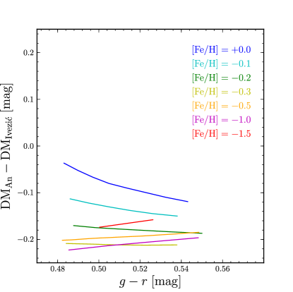
Figure 1.— Comparison between distance moduli derived from the Ivezić et al. (2008) photometric distance relation (their eqn. A7), and those derived from the An et al. (2009) theoretical isochrones.

We select G-type dwarfs by selecting stars with log g $>4.2$, to eliminate giant stars (we have verified that more conservative log g cuts give the same results, see Appendix C). We perform no other cuts (e.g., other color cuts or distance cuts) beyond these basic cuts in order to preserve a relatively simple spatial selection function. This sample contains about 28,000 stars, 23,767 of which lie within the well-populated bins in the ($[\mathrm{Fe/H}]$,$[\alpha\mathrm{/Fe}]$) plane that we analyze below. Distances to individual stars are obtained from the Ivezić et al. (2008) photometric color–metallicity-absolute-magnitude relation (their eqn. A7) applied to the $g-r$ color, rather than the $g-i$ color, using

$$r-i=\frac{(g-r-0.12)}{2.34}\,,$$ (1)

and employing the spectroscopic metallicity. These distances are about 10 percent larger than the distances obtained from the An et al. (2009) stellar isochrones, with little to no color or metallicity dependence over the color and metallicity ranges considered here (see Figure 1 and further discussion in $\mathsection$ 5). Individual distance uncertainties are typically $\lesssim$ 10 percent, and thus do not greatly smooth the underlying Galactic density, whose scales are much larger than this (for an illustration of this see Jurić et al. 2008, where much larger distance uncertainties of around 20 percent were shown to influence the inferred scale heights by less than 5 percent).

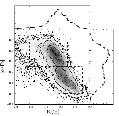
Figure 2.— Distribution of the spectroscopic sample of G dwarfs in elemental-abundance space. The density is linear, and the contours contain 68, 95, and 99 percent of the distribution. Outliers beyond 99 percent are individually shown. Our cuts to select $\alpha$-old (top, left) and $\alpha$-young (bottom, right) samples are shown as dashed boxes. The dotted lines indicate the median [Fe/H] for the $\alpha$-old sample (rounded to the nearest 0.05 dex), used to split the $\alpha$-old sample in [Fe/H], and for $[\alpha\mathrm{/Fe}]$ $<$ 0.25 the dotted box indicates the metal-poor $\alpha$-young sample, used in $\mathsection$$\mathsection$ 4.1 and 4.2.

The distribution of the G-dwarf sample in the elemental abundance space, made up of [Fe/H] and [$\alpha$/Fe], is shown in Figure 2. This distribution is characterized by two modes, one a metal-poor, $\alpha$-enhanced population that must represent the oldest part of the Galactic disk, and another that is metal-rich and has a solar [$\alpha$/Fe] ratio. The two boxes delineated by dashed lines constitute our broad separation of these two populations, which we will refer to as $\alpha$-old and $\alpha$-young, respectively

$$\alpha\text{-}\mathrm{old\ sample}:\qquad\qquad\qquad$$

$$\qquad-1.5<[\mathrm{Fe/H}]<-0.25,\, 0.25<[\alpha\mathrm{/Fe}]<0.50\,,$$ (2)

$$\alpha\text{-}\mathrm{young\ sample}:\qquad\qquad\ \$$

$$\qquad-0.3<[\mathrm{Fe/H}]<\phantom{-}0.25,\, 0.00<[\alpha\mathrm{/Fe}]<0.25\,.$$ (3)

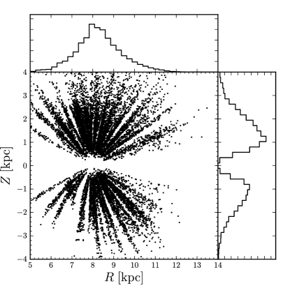
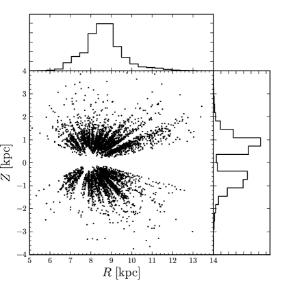
Figure 3.— Spatial distribution of the spectroscopic sample of $\alpha$-old (top panel) and $\alpha$-young (bottom panel) G dwarfs in the $R,Z$ plane.

The spatial distributions of the $\alpha$-old and $\alpha$-young G-dwarf samples are shown in Figure 3, without accounting for the selection function. It is clear from this figure that the bright limit of the G-dwarf sample ($r>14.5$, see below) is such that the effective minimum distance is approximately 600 pc. This means that for the thinner disk components, stars within one scale height are not sampled by SDSS/SEGUE (this is also apparent in Figure 2, where most stars have sub-solar metallicities). However, because the thinner components also contain the most stars (see below and Bovy et al. 2012a), there are still sufficient stars above one scale height of these components such that the G-dwarf data set contains a large number of them.

Understanding and modeling the SEGUE selection function, i.e., the relation between the stars with successfully determined spectral parameters that enter our sample, and their photometric or volume-complete parent population, is central to any analysis that involves the spatial structure of spectroscopically-selected samples. It has not been worked out previously, and while in principle straightforward, it requires attention to a number of details. We describe our model for the SEGUE selection function in Appendix A. The SEGUE G-star sample was obtained by uniformly sampling the dereddened color–magnitude boxes with color range 0.48 $\leq g-r\leq 0.55$ and a “bright” (14.5 $\leq r\leq 17.8$) and “faint” (17.8 $\leq r\leq 20.2$) apparent magnitude range along a set of $\approx 150$ lines of sight. Due to our signal-to-noise ratio cut, this uniform sampling is truncated at a brighter magnitude, where the cut-off is different for each line of sight. We determine the cut-off for each SEGUE plug-plate (which we refer to simply as “plates” in what follows) as the faintest star in the color–magnitude box, and model the $r$-dependence of the selection function using a hyperbolic-tangent step around the cut-off. We obtain the overall selection fraction for each line of sight by comparing the size of the spectroscopic sample to that of the photometric sample in the targeted color–magnitude box for each individual line of sight. This model is described in more detail in Appendix A.

3. Density fitting methodology

3.1. Generalities

Fitting the spatial-density profiles of various G-dwarf sub-samples must account for the fact that the observed star counts do not reflect the underlying stellar distribution, but are strongly shaped by (a) the strongly position-dependent selection fraction of stars with spectra (see Figure 11), (b) the need to use photometric distances that in turn depend on the color and metallicity distribution of the sample (as the magnitude-limited SEGUE sample corresponds to a color- and metallicity-dependent distance-limited sample), and (c) the pencil-beam nature of the SEGUE survey. To properly take all of these effects into account, we need to use forward modeling: in what follows we fit stellar-density models to the data by generating the expected observed distribution of stars in the spectroscopic sample, based on our model for the SEGUE selection function and the photometric distance relation; this predicted distribution is then compared to the observed star counts. We show below how this can be expressed as a maximum likelihood problem. This general density-fitting methodology applies to any spectroscopic survey, with minor modifications, and needs to be applied to obtain selection-corrected distributions from spectroscopically selected stellar samples. In particular, this methodology needs to be applied to constrain the structural parameters of abundance-selected samples in the Milky Way.

As the photometric distance estimates depend on the $g-r$ color, metallicity [Fe/H], and apparent $r$-band magnitude, and because the selection function is a function of position, $r$, and $g-r$, we need to model the observed density of stars in color–magnitude–metallicity–position space, $\lambda(l,b,d,r,g-r,[\mathrm{Fe/H}])$. This density of stars can be written as

$$\begin{split}\lambda(l,b,d,r,&g-r,[\mathrm{Fe/H}])=\\ &\rho(r,g-r,[\mathrm{Fe/H}]|R,Z,\phi)\times\nu_{*}(R,Z,\phi)\\ &\times|J(R,Z,\phi;l,b,d)|\times S(\mathrm{plate},r,g-r)\,.\end{split}$$ (4)

Here, $(R,Z,\phi)$ are Galactocentric cylindrical coordinates corresponding to rectangular coordinates $(X,Y,Z)$, which can be calculated from $(l,b,d)$. The factor $\rho(r,g-r,[\mathrm{Fe/H}]|R,Z,\phi)$ is the number density in magnitude–color–metallicity space as a function of position (see further discussion in Appendix B). The $|J(R,z;l,b,d)|$ is a Jacobian term because of the $(X,Y,Z)\rightarrow(l,b,d)$ coordinate transformation; the crucial factor $S(\mathrm{plate},r,g-r)$ is the selection function as given in equation (A2). Finally, $\nu_{*}(R,Z,\phi)$ is the underlying spatial number density of the sample; we stress that this is a density as a function of rectangular coordinates $(X,Y,Z)$ that we evaluate through $(R,Z,\phi)$ (as we will assume later that the density is axisymmetric), i.e., its dimension is 1 / (spatial unit)³. In what follows we will assume that our models for this density (e.g., exponentials in the vertical and radial direction) are characterized by a set of parameters denoted as $\theta$ and that the density is axisymmetric, such that $\nu_{*}\equiv\nu_{*}(R,Z|\theta)$.

The likelihood of a given model for the density $\nu_{*}(R,z|\theta)$ is given by that of a Poisson process with rate parameter $\lambda$

$$\begin{split}\ln&\mathcal{L}=\sum_{i}\left[\ln\lambda(\{l,b,d,r,\right.\left.g-r,[\mathrm{Fe/H}]\}_{i}|\theta)\right]\\ &-\int\mathrm{d}l\,\mathrm{d}b\,\mathrm{d}d\,\mathrm{d}r\,\mathrm{d}(g-r)\,\mathrm{d}[\mathrm{Fe/H}]\,\lambda(l,b,d,r,g-r,[\mathrm{Fe/H}]|\theta)\,,\end{split}$$ (5)

where the integral is over the domain surveyed and $i$ indexes the observed objects. Because the Jacobian, the selection function, and the density in magnitude–color–metallicity space only enter $\lambda$ multiplicatively (equation (4)) their contribution to the first term ($\ln\lambda$) in equation (5) is a constant that does not depend on the density parameters. Thus, up to a term that does not depend on $\theta$, the log likelihood is equivalent to

$$\begin{split}\ln\mathcal{L}&=\sum_{i}\left[\ln\nu_{*}(R,z|\{l,b,d\}_{i},\theta)\right]\\ &\ -\int\mathrm{d}l\,\mathrm{d}b\,\mathrm{d}d\,\mathrm{d}r\,\mathrm{d}(g-r)\,\mathrm{d}[\mathrm{Fe/H}]\,\lambda(l,b,d,r,g-r,[\mathrm{Fe/H}]|\theta)\,.\end{split}$$ (6)

Note that the Jacobian, the density in the magnitude–color–metallicity space, and the selection function only enter through the second term, and do not need to be evaluated on a star–by–star basis. The second term in equation (6)—the normalization integral—can be written as (assuming that the density does not depend on $(l,b)$ over the area of a plate, although this can easily be relaxed)

$$\begin{split}\int&\mathrm{d}l\,\mathrm{d}b\,\mathrm{d}d\,\mathrm{d}r\,\mathrm{d}(g-r)\,\mathrm{d}[\mathrm{Fe/H}]\,\lambda(l,b,d,r,g-r,[\mathrm{Fe/H}]|\theta)\\ &=A_{p}\,\sum_{\mathrm{plates}\ p}\int\mathrm{d}(g-r)\,\mathrm{d}[\mathrm{Fe/H}]\,\mathrm{d}r\,S(p,r,g-r)\\ &\qquad\int\mathrm{d}d\,\rho(r,g-r,[\mathrm{Fe/H}]|R,Z,\phi)\,d^{2}\,\nu_{*}(R,z|l,b,d,\theta)\,,\end{split}$$ (7)

where $A_{p}$ is the area of a SEGUE plate (approximately 7 deg²).

In the following, we analytically marginalize over the amplitude of the rate $\lambda$ with a logarithmically flat prior. In that case, the log likelihood becomes

$$\begin{split}\ln&\mathcal{L}=\\ &\sum_{i}\left[\ln\nu_{*}(R,z|\{l,b,d\}_{i},\theta)\right.\\ &\left.-\ln\int\mathrm{d}l\,\mathrm{d}b\,\mathrm{d}d\,\mathrm{d}r\,\mathrm{d}(g-r)\,\mathrm{d}[\mathrm{Fe/H}]\,\lambda(l,b,d,r,g-r,[\mathrm{Fe/H}]|\theta)\right]\,.\end{split}$$ (8)

Note that the normalization integral is now moved inside of the logarithm.

In Appendix B, we discuss how we include the magnitude–color–metallicity factor $\rho(r,g-r,[\mathrm{Fe/H}]|R,Z,\phi)$ in the likelihood.

3.2. Stellar number density models

We fit number-density models for the various abundance sub-populations, consisting of a disk with an exponential profile in both the vertical and radial direction, plus a constant density

$$\begin{split}\nu_{*}(&R,Z)=\\ &N(R_{0})\left[\frac{1}{2\,h_{z}}\,\exp\left(-\frac{R-R_{0}}{h_{R}}\right)\,\exp\left(-\frac{|Z|}{h_{z}}\right)+\frac{\beta_{c}}{24}\right]\,,\end{split}$$ (9)

where $N(R_{0})$ is the vertically-integrated number density at $R_{0}$. We refer to this model below as a single-exponential disk fit, as in all cases the data imply $\beta_{c}\ll 1$. We also fit combinations of exponential disks as

$$\begin{split}\nu_{*}&(R,Z)=\\ &N(R_{0})\,\left[\frac{1-\beta_{2}}{2\,h_{z}}\,\exp\left(-\frac{R-R_{0}}{h_{R}}\right)\,\exp\left(-\frac{|Z|}{h_{z}}\right)\right.\\ &\left.+\frac{\beta_{2}}{2\,h_{z,2}}\,\exp\left(-\frac{R-R_{0}}{h_{R,2}}\right)\,\exp\left(-\frac{|Z|}{h_{z,2}}\right)\right]\,.\end{split}$$ (10)

In particular in the $Z$ direction, this is analogous to traditional density fits based on photometric data, which require (at least) two exponential components. We do not fit for the overall normalization, $N(R_{0})$, as we are interested primarily in the shape of the stellar-density profile.

To determine the best-fit parameters and their uncertainties we use Powell’s method for minimization (Press et al., 2007), and then MCMC-sample the posterior distribution function, obtained by multiplying the likelihood in equation (8) with flat logarithmic priors for the scale parameters ($h_{z}$, $h_{R}$, $h_{z,2}$, $h_{R,2}$) and flat priors on the contamination-fraction parameters ($\beta_{c}$, $\beta_{2}$), using an ensemble MCMC sampler (Goodman & Weare 2010; Foreman-Mackey et al., 2011, in preparation).

3.3. Tests on mock data

In Appendix D, we discuss tests of the fitting methodology on mock data sets made up of single-exponential disk components observed using the SEGUE sampling. These tests show that we can recover the input density structure to within the MCMC-determined uncertainties over the range of inferred scale heights, scale lengths, and sample sizes found below.

4. Density structure

First, we briefly discuss the result of fitting the broad bins in abundance as defined in equation (2), in order to explore the broad trends in spatial structure with elemental abundance. In $\mathsection$ 4.3, we then split the sample finely in elemental-abundance space and map the structure of mono-abundance populations.

4.1. The $\alpha$-old stars

Table 1

Table 2Results for the $\alpha$-old G-dwarf sample ( $-1.5<$ [Fe/H] $<-0.25$, $0.25<$ $[\alpha\mathrm{/Fe}]$ $<0.50$)

	$h_{z}$		$h_{R}$		$h_{z,2}$		$h_{R,2}$		$\beta_{2}$		$\beta_{c}$
	(pc)		(kpc)		(pc)		(kpc)
all plates	701	$\pm$5	2.06	$\pm$0.03	…		…		…		0.0000	$\pm$0.0009
bright plates	769	$\pm$14	1.79	$\pm$0.05	…		…		…		0.004	$\pm$0.009
faint plates	714	$\pm$11	2.25	$\pm$0.05	…		…		…		0.001	$\pm$0.001
$b<0^{\circ}$	694	$\pm$9	2.02	$\pm$0.05	…		…		…		0.0000	$\pm$0.0010
$b>0^{\circ}$	699	$\pm$8	2.10	$\pm$0.04	…		…		…		0.000	$\pm$0.001
$|b|>45^{\circ}$	696	$\pm$6	2.23	$\pm$0.06	…		…		…		0.0000	$\pm$0.0009
$|b|<45^{\circ}$	640	$\pm$10	2.05	$\pm$0.04	…		…		…		0.002	$\pm$0.002
all plates	686	$\pm$11	2.01	$\pm$0.05	933	$\pm$49	3.0	$\pm$0.4	0.04	$\pm$0.03	…
bright plates	764	$\pm$20	1.78	$\pm$0.04	3126	$\pm$271	$>$64		0.01	$\pm$0.02	…
faint plates	688	$\pm$40	2.2	$\pm$0.1	1311	$\pm$189	$>$3.0 (5	$\pm$1)	0.03	$\pm$0.04	…
$b<0^{\circ}$	671	$\pm$22	1.97	$\pm$0.08	993	$\pm$169	3.7	$\pm$0.4	0.05	$\pm$0.05	…
$b>0^{\circ}$	687	$\pm$11	2.06	$\pm$0.07	886	${}^{+350}_{-708}$	3	$\pm$1	0.04	$\pm$0.04	…
$|b|>45^{\circ}$	692	$\pm$11	2.2	$\pm$0.1	800	$\pm$88	4.3	$\pm$0.4	0.01	$\pm$0.07	…
$|b|<45^{\circ}$	639	$\pm$17	2.03	$\pm$0.07	1142	$\pm$99	$>$5		0.01	$\pm$0.02	…
[Fe/H] $<$ -0.7	856	$\pm$20	2.06	$\pm$0.08	865	$\pm$108	2.1	$\pm$0.3	0.07	$\pm$0.08	…
[Fe/H] $>$ -0.7	583	$\pm$16	1.97	$\pm$0.08	873	$\pm$62	4.0	$\pm$0.5	0.03	$\pm$0.04	…
0.25 $\leq$ [$\alpha$/Fe] $<$ 0.35	627	$\pm$18	2.23	$\pm$0.10	802	$\pm$104	3.5	$\pm$0.3	0.03	$\pm$0.06	…
0.35 $\leq$ [$\alpha$/Fe] $<$ 0.50	765	$\pm$15	1.89	$\pm$0.04	826	$\pm$45	2.0	$\pm$0.1	0.03	$\pm$0.06	…

Note. — Lower limits are at 99 percent posterior confidence. Lower limits are given when the best-fit value is larger than 4.5 kpc. The best-fit value is not given if the best-fit value is larger than 6 kpc.

For the $\alpha$-old sample, the fit results for single exponential profiles in $R$ and $Z$, and for a combination of two exponential profiles for both $R$ and $Z$, are given in Table 2. The model with two exponentials in both $R$ and $Z$ is preferred, but the parameters of the dominant double-exponential disk are similar for both fits. That is, even when we give the model the additional freedom of two vertical scale heights, the data lead us to employ only a single exponential scale height. There is no evidence for a thinner component in the $\alpha$-old abundance range. We see that the $\alpha$-old sample is dominated by a population of stars with a scale height of 686$\pm$11 pc, and a short scale length of 2.01$\pm$0.05 kpc (consistent with the rough estimate of 2 kpc based on a handful of stars by Bensby et al. 2011 and the indirect dynamical estimate of 2.2$\pm$0.35 kpc of Carollo et al. 2010).

We have split the $\alpha$-old sample into more metal-poor and more metal-rich sub-samples by cutting the sample at [Fe/H] = $-0.7$. This is close to the median [Fe/H] of the $\alpha$-old sample. The metal-poor sub-sample may be identified with the metal-weak thick disk (MWTD) population discussed by Carollo et al. (2010), which they argue covers the metallicity range $-1.8\leq[\mathrm{Fe/H}]\ \leq-0.8$. The resulting fits for the spatial structure of these sub-samples are given in Table 2. The inferred scale lengths for these sub-samples are equal to within the uncertainties. However, the scale height of the more metal-poor sample is 856$\pm$20 pc while that of the more metal-rich sample is 583$\pm$16 pc. The radial scale length of the MWTD determined from the indirect dynamical analysis of Carollo et al. (2010) is roughly 2 kpc, while the scale height is 1.36$\pm$0.13 kpc.

We have also split the $\alpha$-old sample into two bins in $[\alpha\mathrm{/Fe}]$ by splitting the sample at $[\alpha\mathrm{/Fe}]$ = 0.35. The best-fit density profiles, given at the bottom of Table 2, again have similar scale lengths, around 2 kpc, and different scale heights. The stars that are most enhanced in $\alpha$-elements have the largest scale height (765$\pm$15 pc) and the shortest scale length (1.89$\pm$0.04 kpc), while the less $\alpha$-enhanced stars have a smaller scale height (627$\pm$18 pc) and longer scale length (2.23$\pm$0.1 kpc). As the latter dominate the full $\alpha$-old sample, their scale height is very similar to that inferred for the full sample. We explore the dependence of the disk parameters on $[\mathrm{Fe/H}]$ and $[\alpha\mathrm{/Fe}]$ in more detail in $\mathsection$ 4.3 below.

4.2. The $\alpha$-young sample

The results for single exponential disk fits and double exponential disk fits for the $\alpha$-young sample are given in Table 4. The double exponential disk fit model is formally preferred, but the parameters of the dominant double-exponential disk are again similar for both fits. We see that the $\alpha$-young sample is dominated by a population of stars with a low scale height of 256$\pm$4 pc and a long scale length of 3.6$\pm$0.2 kpc.

The second double-exponential disk in the best-fit model for the $\alpha$-young sample has a scale height of 664$\pm$132 pc, which is consistent with the scale-height measurement of the $\alpha$-old sample above. However, the fraction of stars in this secondary component is too small to constrain its scale length, and is conceivably simply a result of ‘abundance contamination’ of the sample.

Density fits for $\alpha$-young samples with the same $[\alpha\mathrm{/Fe}]$ limits as the nominal $\alpha$-young sample shown in the top panel, but that are more metal-poor, are also given in Table 4. We do not measure any radial density decline for these more metal-poor $\alpha$-young samples, and short scale lengths for these samples are ruled out by the data. We consider this further in $\mathsection$ 4.3 and in the discussion section below.

When we split the $\alpha$-young sample into two pieces, by cutting at $[\alpha\mathrm{/Fe}]$ = 0.15, we find that the more $\alpha$-enhanced sample has the shortest scale length (2.3$\pm$0.2 kpc) and the largest scale height (348$\pm$13 pc). The sample with $[\alpha\mathrm{/Fe}]$ closer to solar has a longer scale length of 4.3$\pm$0.2 kpc and a smaller scale height of 239$\pm$4 pc.

Table 3

Table 4Results for the $\alpha$-young G-dwarf sample ( $-0.3<$ [Fe/H] $<0.25$, $0.00<$ $[\alpha\mathrm{/Fe}]$ $<0.25$)

	$h_{z}$		$h_{R}$		$h_{z,2}$		$h_{R,2}$		$\beta_{2}$		$\beta_{c}$
	(pc)		(kpc)		(pc)		(kpc)
all plates	270	$\pm$3	3.8	$\pm$0.2	…		…		…		0.0005	$\pm$0.0010
bright plates	267	$\pm$3	3.6	$\pm$0.2	…		…		…		0.0009	$\pm$0.0003
faint plates	329	$\pm$14	$>$3.8 (5.1	$\pm$1.0)	…		…		…		0.0010	$\pm$0.0003
$b<0^{\circ}$	264	$\pm$4	3.6	$\pm$0.2	…		…		…		0.0008	$\pm$0.0009
$b>0^{\circ}$	271	$\pm$4	3.80	$\pm$0.10	…		…		…		0.000	$\pm$0.001
$|b|>45^{\circ}$	270	$\pm$5	4.2	$\pm$0.8	…		…		…		0.0004	$\pm$0.0008
$|b|<45^{\circ}$	264	$\pm$3	4.0	$\pm$0.2	…		…		…		0.0006	$\pm$0.0007
all plates	256	$\pm$4	3.6	$\pm$0.2	664	$\pm$132	$>$5		0.012	$\pm$0.004	…
bright plates	260	$\pm$5	3.5	$\pm$0.3	491	$\pm$83	$>$2		0.02	$\pm$0.02	…
faint plates	268	$\pm$23	$>$3.8 (5.0	$\pm$0.8)	910	$\pm$152	$>$2.9 (6	$\pm$2)	0.014	$\pm$0.008	…
$b<0^{\circ}$	242	$\pm$8	3.2	$\pm$0.2	639	$\pm$81	$>$5		0.017	$\pm$0.010	…
$b>0^{\circ}$	263	$\pm$6	3.7	$\pm$0.2	834	$\pm$70	$>$4		0.004	$\pm$0.002	…
$|b|>45^{\circ}$	249	$\pm$6	3.8	$\pm$0.8	631	$\pm$142	$>$6		0.015	$\pm$0.005	…
$|b|<45^{\circ}$	252	$\pm$5	3.9	$\pm$0.3	656	$\pm$65	$>$5		0.012	$\pm$0.005	…
-1.5 $<$ [Fe/H] $<$ -0.6	689	$\pm$25	$>$37		1431	${}^{+704}_{-1916}$	1.1	${}^{+0.6}_{-1.0}$	0.03	$\pm$0.07	…
-0.6 $<$ [Fe/H] $<$ -0.3	360	$\pm$9	$>$16		946	$\pm$92	$>$14		0.018	$\pm$0.009	…
0.00 $<$ [$\alpha$/Fe] $<$ 0.15	239	$\pm$4	4.3	$\pm$0.2	647	$\pm$53	$>$7		0.010	$\pm$0.003	…
0.15 $\leq$ [$\alpha$/Fe] $<$ 0.25	348	$\pm$13	2.3	$\pm$0.2	959	$\pm$335	$>$2.0 (5	$\pm$2)	0.018	$\pm$0.009	…

Note. — Lower limits are at 99 percent posterior confidence. Lower limits are given when the best-fit value is larger than 4.5 kpc. The best-fit value is not given if the best-fit value is larger than 6 kpc.

4.3. The spatial structure of mono-abundance sub-populations

In the previous two sections we found that sub-samples of stars defined by their element abundances appear to have a simple spatial structure, approximated by a single exponential in the radial and vertical direction. The scale lengths and heights of these sub-sets seem to vary systematically with the abundances: the $\alpha$-old sample has a shorter scale length than the $\alpha$-young sample, and if we split those two samples further in $[\alpha\mathrm{/Fe}]$, the part of the $\alpha$-young sample that has the closest to the solar $[\alpha\mathrm{/Fe}]$ ratio has the longest scale length and the smallest scale height. We also noticed that populations with $[\alpha\mathrm{/Fe}]$ $<0.25$ have longer scale lengths and scale heights with decreasing $[\mathrm{Fe/H}]$.

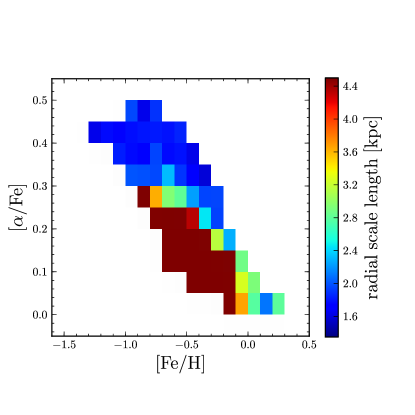
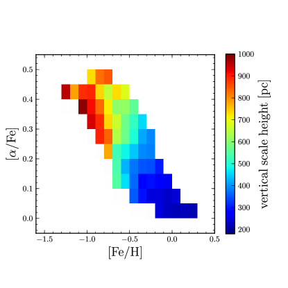
Figure 4.— Radial scale length (left panel) and vertical scale height (right panel) of the best-fitting density models with a single exponential in $R$ and $Z$, shown for different mono-abundance sub-populations as a function of their position in the $[\mathrm{Fe/H}]$ and $[\alpha\mathrm{/Fe}]$ plane. Pixels span 0.1 dex in $[\mathrm{Fe/H}]$ and 0.05 dex in $[\alpha\mathrm{/Fe}]$. Only pixels with more than 100 stars are shown. The striking correlations between the spatial structure and the elemental abundances of the sub-populations is apparent.

To further investigate these trends, we have fit disk models with single exponential profiles in $R$ and $Z$ to sub-populations of stars with narrow bins in $[\mathrm{Fe/H}]$ and $[\alpha\mathrm{/Fe}]$. We divide stars into bins of width 0.1 dex in $[\mathrm{Fe/H}]$ and 0.05 dex in $[\alpha\mathrm{/Fe}]$, and only fit those bins with more than 100 stars. The results from these fits are shown in Figure 4. The populations in the lower left part of the $[\alpha\mathrm{/Fe}]$–$[\mathrm{Fe/H}]$ diagram all have best-fit scale lengths in excess of 4.5 kpc.

We also fit two-component, i.e., two exponential disks to each of the bins, but found that these led to overfitting, and only marginal improvements in the likelihood for the best fit. Thus, for narrow bins in elemental-abundance space, the sub-populations are very-well described by single exponential profiles in the $R$ and $Z$ directions.

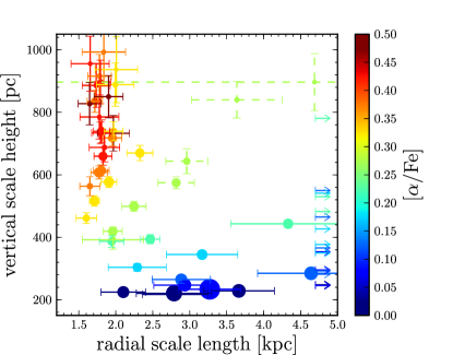
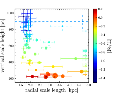
Figure 5.— Correlation between the radial scale length and vertical scale height of mono-abundance sub-populations, essentially a different projection of the results in Figure 4. The top panel shows the vertical scale height versus the radial scale length, color-coded by $[\alpha\mathrm{/Fe}]$. The bottom panel shows the same as the top panel, but with $[\mathrm{Fe/H}]$ color-coding. Bins with best-fit scale lengths in excess of 5 kpc are indicated with lower limits in the bottom row. The area of the disks are proportional to the total surface-mass density contained in each point’s $[\mathrm{Fe/H}]$–$[\alpha\mathrm{/Fe}]$  bin, corrected for mass and sample selection effects (see Bovy et al. 2012a). Some of the uncertainties on the vertical scale heights are smaller than the points. The bins with dashed errorbars lie in a part of the abundance plane where abundance contamination is likely to be most severe, where the $[\alpha\mathrm{/Fe}]$-based age ranking is least reliable, and where the spatial properties change most rapidly. They contain $<$ 5 percent of the disk surface mass.

A different view of the results in Figure 4 is given in Figure 5. The results in the different $[\mathrm{Fe/H}]$–$[\alpha\mathrm{/Fe}]$ bins are shown as a function of scale length and scale height; the points are color-coded by their $[\alpha\mathrm{/Fe}]$ or $[\mathrm{Fe/H}]$ dependence, and the size of the points corresponds to the total stellar surface-mass density—corrected for mass and sample selection effects–in each population (calculated in Bovy et al. 2012a). Figure 5 also shows the uncertainties in the inferred parameters; the formal uncertainty in the scale height for some points is so small that it cannot be seen. The bins with dashed error bars lie in a part of the abundance plane where abundance contamination is likely to be the most severe, where the $[\alpha\mathrm{/Fe}]$-based age ranking is least reliable, and where the spatial properties change most rapidly. They contain $<$ 5 percent of the disk surface mass.

We see that these fits for mono-abundance sub-components flesh out the main trends we noted in the broader $[\mathrm{Fe/H}]$ and $[\alpha\mathrm{/Fe}]$ ranges above. At any given metallicity $[\mathrm{Fe/H}]$, the scale length increases and the scale height decreases when moving from $\alpha$-old to $\alpha$-young populations. At any given $\alpha$-age, the scale length and the scale height increase for the more metal-poor components, implying an outward metallicity gradient. And, as Figure 5 shows most clearly, increasing scale lengths are correlated with decreasing scale heights (except for a few bins on the boundary between the very long scale lengths at low metallicity and solar $\alpha$-enhancement and the shorter scale lengths of the $\alpha$-old populations; see further discussion in $\mathsection$ 5.5). From Figure 4 it is clear that neither $[\alpha\mathrm{/Fe}]$ or $[\mathrm{Fe/H}]$, on its own, accounts for the trends in scale height and scale length. We discuss what this implies for disk formation and evolution in $\mathsection$$\mathsection$ 5.4 and 5.5, respectively.

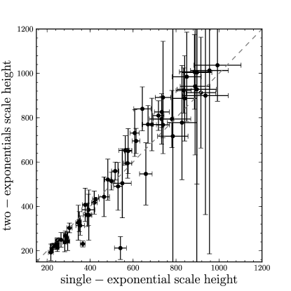
Figure 6.— Scale height of the dominant component, when fitting two exponential components in $R$ and $Z$, versus the scale height for a single exponential component in $R$ and $Z$. The dashed line gives the one–to–one correspondence. For most mono-abundance populations a single exponential description in $Z$ is a good model.

Figure 6 shows the results of fitting two components with exponential profiles in both $R$ and $Z$ to each abundance bin. The scale height of the dominant component is shown against the best-fit scale height, when fitting a single exponential profile in $R$ and $Z$. We see that these scale heights are strongly clustered around the one–to–one correspondence line. Thus, for each bin, a single vertical exponential suffices to explain the observed number counts. The fact that the two measurements agree better than would be expected, given the uncertainties shown, is due to the fact that the scale heights for each bin are strongly correlated when fitting a single or a double exponential profile in $R$ and $Z$. Overall, Figure 6 confirms that a single exponential model in $Z$ and $R$ is a good model for the spatial structure of mono-abundance sub-populations.

In Appendix D, we perform a test to determine whether abundance uncertainties can plausibly lead us to find spurious disk components between a “thin” and a “thick” component. That is, we ask whether it is plausible that an underlying density dominated by distinct thin- and thick-disk components can be smoothed by abundance errors into the density structure we inferred in Figures 4 to 6. This test shows that if this were the case, every bin is preferentially fit with two components, corresponding to the input thin and thick components. The equivalent of Figure 6, shown in the bottom right panel of Figure 20, is qualitatively different, with a distinct difference between the single-component scale height and the scale height of the dominant component in the two-component fit.

To test whether the analysis in this section is influenced by our signal-to-noise ratio cut of SN $>15$, we have repeated the analysis with a cut of SN $>30$, as also used by Lee et al. (2011b). The equivalents of Figures 4 to 6 look qualitatively the same, albeit with larger uncertainties for each bin, and the dependence of $h_{z}$ and $h_{R}$ on elemental abundance is the same as that inferred from the sample with the SN $>15$ cut. The number of ($[\mathrm{Fe/H}]$,$[\alpha\mathrm{/Fe}]$) bins with more than 100 stars is smaller, but the inferred ($h_{z}$,$h_{R}$) for those bins with more than 100 stars when using SN $>30$ cut are consistent within the uncertainties with those found with the less restrictive signal-to-noise ratio cut. We stress that even when selecting stars with SN $>30$, the equivalent of Figure 6 does not show any sign of a second component in the mono-abundance bins.

To perform the binning in this section, we used narrow bins of 0.1 dex in $[\mathrm{Fe/H}]$ and 0.05 dex in $[\alpha\mathrm{/Fe}]$. These bins are somewhat narrower than the total typical uncertainty ($\approx 0.15$ dex in $[\mathrm{Fe/H}]$, $\approx 0.07$ dex in $[\alpha\mathrm{/Fe}]$; Bovy et al. 2012b), but we prefer to oversample, rather than undersample, to avoid smoothing out underlying structure. The analysis in each bin holds irrespective of the bin size. What matters for the analysis is that the data in each bin are disjoint, such that the bins are statistically independent.

5. Discussion

Our basic result is that various stellar disk sub-components, when defined purely through stellar abundances, are simple, i.e., can be described by a single exponential in $R$ and $Z$, and exhibit distinctive trends of the scale height and scale length with chemical abundance. This suggests that dissecting the Milky Way’s disk on the basis of chemical abundances alone is a useful approach. In this section we go through a number of practical issues pertaining to these estimates, before discussing possible implications for galactic disk formation and evolution.

5.1. Distance systematics

The absolute values of the distance scales measured in this paper are subject to distance systematics, which we discuss in this subsection. We have used the data-driven photometric-distance relation from Ivezić et al. (2008) to infer the spatial structure of the various samples of stars, but an alternative photometric-distance relation can be obtained by using the An et al. (2009) stellar isochrones in the SDSS passbands. These isochrones depend on $[\mathrm{Fe/H}]$ as well as on $[\alpha\mathrm{/Fe}]$, although in practice a linear relation between $[\alpha\mathrm{/Fe}]$ and $[\mathrm{Fe/H}]$ is assumed, and the spectroscopically measured $[\alpha\mathrm{/Fe}]$ is not used directly to estimate the photometric distance. In the top panel of Figure 1 we compared the distance moduli derived using the An et al. (2009) stellar isochrones with those obtained using the Ivezić et al. (2008) relation for a few values of $[\mathrm{Fe/H}]$. We see that, for the values of $[\mathrm{Fe/H}]$ that span most of our sample, the distance modulus difference is -0.12 mag, corresponding to a systematic difference in the inferred distances of about 6 percent, nearly independent of color. Thus, if we had used the An et al. (2009) photometric distances we would have obtained scale lengths and scale heights that were 6 percent shorter.

A second distance systematic that could influence our results is the Malmquist bias (Malmquist, 1920, 1922)—the fact that brighter stars are over-represented in a magnitude-limited survey. For our relatively bright sample, this is dominated by the finite width of the photometric distance relation. The Malmquist bias in absolute magnitude is apparent-magnitude dependent and approximately equal to $-\sigma^{2}\mathrm{d}\ln A(r)/\mathrm{d}r$, where $A(r)$ is the differential number count as a function of apparent magnitude and $\sigma$ is the dispersion in the absolute magnitudes (either due to photometric uncertainties or due to intrinsic scatter in the photometric distance relation). Conservatively assuming that the combination of the finite width of the photometric distance relation and the photometric uncertainties is 0.2 mag, and that the underlying density is constant, the Malmquist bias would be of order 2.5 percent. However, due to the exponential fall-off of the density in both the $R$ and $Z$ directions, the differential number counts are (a) flat near the peak induced by the vertical exponential, and (b) for most apparent magnitudes $|\mathrm{d}\ln A(r)/\mathrm{d}r|$ is less than 1. Therefore, the Malmquist bias is at most about 2 percent, and will not strongly affect the measurement of the vertical scale height in particular.

We have assumed throughout our analysis that all of the stars in our sample are single. The presence of unresolved binaries will lead us to underestimate scales, as these binaries will appear to us as brighter, and thus closer, single stars. The binary fraction and companion-mass distribution for G-type dwarfs remains controversial, but it appears that the overall binary fraction for G dwarfs is approximately 40 percent (Abt & Levy, 1976; Duquennoy & Mayor, 1991; Raghavan et al., 2010), similar to but slightly larger than that of M dwarfs (Fischer & Marcy, 1992; Raghavan et al., 2010). The distribution of companion masses is poorly known, and could range from being peaked around 20 percent of the primary’s mass (Duquennoy & Mayor, 1991), to being relatively flat between 20 and 100 percent of the primary’s mass (Raghavan et al., 2010), with numerical simulations indicating that multiple-star systems form preferentially with approximately equal-mass members (Bate, 2005), and an overall multiplicity fraction of around 40 percent (Bate et al., 2003). Lower-metallicity stars most likely have a higher binary fraction (Machida et al., 2009), and could reach 100 percent for $[\mathrm{Fe/H}]$ $<-0.8$ (Raghavan et al., 2010).

For a likely scenario where 40 percent of our $\alpha$-young sample is made up of binary stars (ignoring higher-order multiplicities) with a flat distribution of companion masses between 20  and 100 percent of the primary’s mass, the magnitude would be overestimated on average by 0.12 mag, such that the scale height and scale length would be underestimated by about 6 percent. If 70 percent of the $\alpha$-old sample would consist of binary systems (taking into account the rising binary fraction with decreasing metallicity), the magnitudes would be overestimated by approximately 0.21 mag, and the $\alpha$-old scale heights and scale lengths would be underestimated by 10 percent. These biases are somewhat larger than the statistical uncertainties on our results, but they are similar to the overall distance-scale uncertainty (see above), and they do not change the conclusion that the $\alpha$-old scale length is much shorter than that of the $\alpha$-young sample. Even in a worst-case scenario, where all binary systems have equal-mass companions and where 100 percent of the $\alpha$-old stars are in binaries, the $\alpha$-old scale-length would still be $\lesssim 2.8$ kpc (40 percent up from 2 kpc), which is shorter than the scale length measured for the $\alpha$-young sample in Table 4 and Figure 5, and the $\alpha$-young scale lengths themselves would also increase by about 15 percent in this scenario. In principle, a careful spectral analysis of the SEGUE spectra itself could provide direct constraints on the (unresolved) binary contamination in this sample.

5.2. Halo contamination

In our density fits we have mostly fit disk components to the data, except for the single exponential disk model where we added a uniform density (equation (9)). We thus assumed that the stellar halo does not influence our disk fits, beyond what can be described by a uniform density across our survey volume. We can estimate the expected number of halo stars in our sample using the Bell et al. (2008) density fits to the smooth stellar halo. We run the Bell et al. (2008) stellar-halo density through the G-star SEGUE selection function, and marginalize over $g-r$ color using a flat distribution over $0.48\leq g-r\leq 0.55$, and over $[\mathrm{Fe/H}]$ using the Ivezić et al. (2008) halo metallicity distribution (mean $[\mathrm{Fe/H}]$ = -1.52, width = 0.32). We then find that for $\approx 10^{8}$ G-type stars between 1 and 40 Galactocentric kpc in the stellar halo, there should be about 100 halo stars in our sample, compared to the total sample size of 30,353 G-type dwarfs. Hence, the halo contamination is very small and does not influence the fits. Additionally, halo contamination will be most severe for the $\alpha$-old sub-populations, and this contamination should work to increase the inferred scales (length and height). Therefore, the result that the radial scale length of $\alpha$-old sub-populations is shorter than that of $\alpha$-young sub-populations is robust against any halo contamination.

5.3. Comparison to traditional geometric disk decompositions

The density fits in this paper are the first to constrain the vertical scale height and radial scale length of numerous disk sub-components, defined using elemental abundances alone, from a large sample of stars. Our results show that the vertically thicker disk sub-components—when chemically defined—have a much shorter scale length than the thinner-disk sub-components, which is opposite to traditional purely geometric disk decompositions (e.g., Robin et al., 1996; Ojha, 2001; Larsen & Humphreys, 2003), which typically find that the thick-disk component has a longer scale length than the thin disk, and that this scale length is $\gtrsim 3.5$ kpc (e.g., Jurić et al., 2008).

When we fit the spatial structure in our approach, taking stars of all metallicities (specifically, the combination of our $\alpha$-old (“thick”) and $\alpha$-young (“thin”) samples), we can recover the result of purely geometric decompositions: the thin-disk component—i.e., the component with the lowest scale height, $\approx$ 300 pc—gets paired with the shortest scale length ($\approx$ 2 kpc), while the thicker-disk component gets assigned both the largest scale height and scale length (for our particular sample fit with a combination of three double-exponential disks these are $\approx$ 600 pc and $\approx$ 2.4 kpc, with a small component with an even larger scale height and scale length). Thus, it seems that purely geometric decompositions naturally associate the longest scale length with the largest scale height. That both geometrically determined scale lengths are shorter than the scale length of the $\alpha$-young sample is due to the fact that the metallicity distribution for the entire sample extends down to $[\mathrm{Fe/H}]$ = -1.5, such that the model ‘expects’ many low-metallicity stars in the “thin” component at large distances (as the model does not contain the information that the thin component has higher metallicities), which are not observed. Therefore, metallicity and $\alpha$-element abundances, which are manifestly quantities that can identify sub-samples of stars independent of their spatial structure and kinematics, lead to a qualitatively different decomposition into two (or more) sub-components than the purely geometrical approach, with its inherent risk of circular reasoning.

5.4. Implications for disk formation

The distinctive changes of the global disk structure with abundance, especially with the age proxy $[\alpha\mathrm{/Fe}]$, should provide valuable clues to the formation of the Milky Way’s disk. While a concrete and quantitative model comparison is beyond the scope of this paper, we discuss some of the qualitative implications here. As mentioned in Section 1, the overall radial-density profile of the stellar disk is expected to be conserved even in the face of large-scale radial migration, but the radial profile of sub-components will tend to relax to the mass-weighted mean radial profile. Thus, a difference in the radial distribution of various populations of stars today is a less-pronounced version of more different initial radial distributions (at formation). Assuming that the $[\alpha\mathrm{/Fe}]$ ratio is an adequate proxy for age (e.g., Schönrich & Binney, 2009b), our results then imply that the $\alpha$-enhanced, hence oldest, populations are more centrally concentrated—have a shorter scale length—than populations with $\alpha$-abundances that are closer to Solar, and therefore younger. This is direct observational evidence for inside-out formation of galactic disks across the presumed age range of our sample, 1 – 10 Gyr, where the inner parts of the disk form before the outer part of the disk. A similar age-dependence of the exponential scale length has been found in several external galaxies (de Jong et al., 2007; Radburn-Smith et al., 2012).

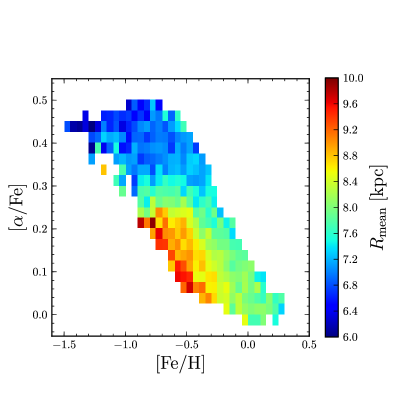
Figure 7.— Mean orbital radii of the G-dwarf sample. Median values of the mean orbital radii are shown, in bins of width 0.05 dex in $[\mathrm{Fe/H}]$ and 0.025 dex in $[\alpha\mathrm{/Fe}]$. Only bins with at least 20 stars are shown.

Second, our analysis shows that our Milky Way has not only a metallicity gradient among its youngest stars, but that it has always had one (Cheng et al., 2011): at a given $[\alpha\mathrm{/Fe}]$, standing in for age, sub-populations with lower $[\mathrm{Fe/H}]$ have a longer scale length than more metal-rich stars. This picture is confirmed by looking at the orbital properties of the stars when integrating our sample of G-type dwarfs in a simple model for the Milky Way’s potential, made up of a Miyamoto-Nagai disk with a radial scale of 4 kpc and vertical scale of 300 pc contributing 60 percent of the radial force at the Solar radius, a Hernquist bulge with a scale radius of 600 pc contributing 5 percent of the radial force, and a Navarro-Frenk-White halo with a scale radius of 36 kpc that contributes 35 percent of the rotational support at the Sun’s position. The median of the mean orbital radii as a function of elemental abundance is shown in Figure 7 (see also Lee et al. 2011b and Liu & van de Ven, 2011, in prep. for similar figures of the eccentricity and rotational velocity). We see that stars with $[\alpha\mathrm{/Fe}]$ $<0.25$ and lower $[\mathrm{Fe/H}]$ are thin-disk stars that live, on average, farther out than more metal-rich stars. Thus, the longer scale length for outer-disk stars, combined with the fact that, for solar $[\alpha\mathrm{/Fe}]$  decreasing $[\mathrm{Fe/H}]$ is correlated with decreasing age (e.g., Schönrich & Binney, 2009b), implies that the outer part of the disk formed later than the inner part.

We have assumed that $[\alpha\mathrm{/Fe}]$ is an adequate proxy for age, such that the mono-abundance populations that are more $[\alpha\mathrm{/Fe}]$-enhanced are older than the populations with solar $[\alpha\mathrm{/Fe}]$. This is typically the case in standard scenarios for the star formation history of the Milky Way disk, in which $[\alpha\mathrm{/Fe}]$ steeply drops around 2 to 3 Gyr due to the onset of type Ia supernovae (Dahlen et al., 2008; Maoz et al., 2011), and then stays roughly constant, although the value of $[\mathrm{Fe/H}]$ at which the $[\alpha\mathrm{/Fe}]$ downturn happens depends on the star formation history (Matteucci & Recchi, 2001). Only if the local star formation was characterized by bursts of star formation can younger populations of stars have similar levels of $[\alpha\mathrm{/Fe}]$ as older stars (Gilmore & Wyse, 1991). Most current fits of the local star formation history prefer a smooth history (e.g., Aumer & Binney, 2009), although it is difficult to rule out epochs of enhanced star formation (e.g., Rocha-Pinto et al., 2000).

5.5. Implications for disk evolution

The spatial structure inferred for mono-abundance sub-populations (Figures 4 and 5) show two important results: first, there is a tight anti-correlation between the scale heights and scale lengths of the sub-components. Secondly, there is a continuous distribution in scale height when moving from $\alpha$-enhanced, metal-poor populations to stars with solar $[\alpha\mathrm{/Fe}]$ and $[\mathrm{Fe/H}]$. This suggests that the $\alpha$-old—“thick”—and the $\alpha$-younger, “thin”, regime of the stellar disk are not two separate entities, but merely opposite ends of the disk evolution spectrum (suggested before in Norris, 1987, but never directly measured as we do here). This issue, which requires proper stellar-mass weighting of the sub-components, is worked out in a separate paper (Bovy et al., 2012a). Taken together, these findings suggest a continuous evolutionary mechanism created the observed scale-height distribution, rather than a discrete external heating or accretion event. Radial migration is an obvious candidate for this internal evolution mechanism. That the most centrally concentrated component of the disk is not only the ($\alpha$-)oldest part, but also has the largest scale height, is a nearly inevitable condition, and hence a natural prediction, of any scenario where much of the disk scale-height distribution is created through radial migration. The $\alpha$-old sub-population not only had the most time to evolve, but its centrally concentrated parent population implies that stars at $6<R<12$ kpc have migrated out by the largest factor.

A different internal explanation for the thicker disk components in the Milky Way is that, rather than being thickened over the history of the Galactic disk, thick components were created thick during an early, turbulent phase in the formation of the disk (e.g., Bournaud et al., 2009; Förster Schreiber et al., 2009). If such a scenario is combined with a inside-out growth of the disk, and the disk remains turbulent over a significant fraction of its history, this formation scenario could plausibly explain the continuous dependence of disk structure on elemental abundance found in this paper.

Our result that the transition between the $\alpha$-young, “thin”, components and the $\alpha$-old, “thick”, components is smooth, rather than showing a clear separation between thin and thick components, may appear to be in conflict with local, high-resolution spectroscopic samples of stars (e.g., Reddy et al., 2006; Fuhrmann, 2011; Navarro et al., 2011) or other analyses of the SEGUE data (e.g., Lee et al., 2011b). A detailed comparison between these and our results requires careful accounting for the spectroscopic volume sampling, which has not been done in the Lee et al. (2011b) analysis or for the high-resolution samples, except for the sample of Fuhrmann (2011), which is volume complete out to 25 pc. Without taking the volume selection into account, the sample used here also displays a bi-modality in the $[\mathrm{Fe/H}]$–$[\alpha\mathrm{/Fe}]$ plane (see Figure 2). We discuss this issue in more detail in Bovy et al. (2012a), but we note here that the apparent bi-modality in the observed number density of stars disappears when properly correcting for the spectroscopic sampling. Furthermore, the local, high-resolution analyses cannot directly measure the spatial distribution of stars of different elemental abundances (e.g., Fuhrmann 2011, which only has 15 high-$[\alpha\mathrm{/Fe}]$ stars out to 25 pc; Reddy et al. 2006) and therefore rely on kinematics to argue that the vertical distribution of stars in the Solar neighborhood is characterized by a bi-modal “thin”–“thick”-disk dichotomy. This interpretation is driven by the selection of stars that are disjoint in $[\alpha\mathrm{/Fe}]$, which leads to disjoint kinematics because the kinematics is a strong—and smooth—function of abundance as well (Bovy et al., 2012b). While the stellar content of different survey volumes can (and should) be connected by dynamics, we note that the effective volumes sampled by, e.g., the Fuhrmann (2011) survey and by our analysis differ by a factor of about $10^{5}$; hence the extrapolation from one to the other is enormous. The analysis of the vertical kinematics of stars in our sample confirms the existence of the intermediate populations with scale heights between 400 and 600 pc and vertical-velocity dispersions of 30 to 35 km s^-1 (Bovy et al., 2012b).

Our finding that the scale length does not behave as smoothly as the scale height, as a function of $[\alpha\mathrm{/Fe}]$, is presumably a consequence of the disk’s formation history: here the increasing metallicity as a function of time (i.e., youth) and the radial metallicity gradient compete. As the mapping between $[\alpha\mathrm{/Fe}]$ and age is not linear, but rather, $[\alpha\mathrm{/Fe}]$ steeply drops around 2 to 3 Gyr due to the onset of type Ia supernovae (Matteucci & Recchi, 2001; Dahlen et al., 2008; Maoz et al., 2011), and then stays roughly constant, the scale length should change similarly rapidly with $[\alpha\mathrm{/Fe}]$. The scale height, however, is determined by subsequent evolution, where radial migration transports stars to larger Galactocentric radii, where the lower disk density allows them to travel farther from the plane. Since this evolution is continuous, rather than sudden, and includes additional contributions from heating, trends in scale height versus elemental abundance should be expected to be smoother, even if radial migration is not the disk’s dominant evolutionary mode. Our results are therefore consistent with a scenario where the thick-disk component is the inner part of the disk that formed at the earliest time, and either by having formed thick or through the effect of radial migration, has a large scale height at the present time.

A gas-rich merger, followed by intense star formation at an early time, could have affected the formation of the early disk (Brook et al., 2004), as seems consistent with the observed distribution of eccentricities of the thick-disk component (Sales et al., 2009; Dierickx et al., 2010; Wilson et al., 2011). However, it would lead to a scale length for the thicker component that is larger than that of the thinner component (Qu et al., 2011). It is clear that internal mechanisms must have played an important role during the evolution of the disk. However, we caution that the radial and vertical consequences of neither radial migration, nor turbulent disk evolution, nor of satellite thickening, have been worked out in quantitative detail, and, in particular, resonant coupling between satellites and the disk might induce some similar observational signatures to radial migration.

The rapid change in the mean stellar population in an $[\alpha\mathrm{/Fe}]$– $[\mathrm{Fe/H}]$ abundance bin at the onset of type Ia supernovae is also likely the explanation for the presence of the few points of intermediate $[\alpha\mathrm{/Fe}]$ and $[\mathrm{Fe/H}]$ in Figure 5 that do not follow the anti-correlation between scale height and scale length; these bins, which do not contribute significantly to the total stellar mass (indicated by the size of the symbols in Figure 5), are also the bins that fall short of the one-to-one correlation between single- and two-disk fits in Figure 6. This provides further evidence of the fact that at the rapid $[\alpha\mathrm{/Fe}]$ (age) transition our bins do not adequately resolve single components.

6. Conclusions

The main conclusions of this paper are as follows

$\bullet$ An assessment of the global ($R,Z$) structure of the Milky Way’s stellar disk for sub-components selected solely by their elemental abundances is now feasible, e.g., with spectroscopic surveys such as SEGUE, but requires a thorough accounting for the effective selection function of the spectroscopic sample.

$\bullet$ A decomposition of the Galactic disk, based on SDSS/SEGUE data for G-type dwarfs, into mono-abundance sub-populations in the $[\mathrm{Fe/H}]$–$[\alpha\mathrm{/Fe}]$ plane, reveals that each such component has a simple spatial structure that can be described by single exponential profiles in both the vertical and the radial direction.

$\bullet$ Adopting increasing levels of $[\alpha\mathrm{/Fe}]$ enhancement as a proxy for the increasing age of the stellar population, the disk dissection into narrow mono-abundance populations in the space of $[\mathrm{Fe/H}]$ and $[\alpha\mathrm{/Fe}]$ exhibits a continuous trend of increasing scale height and decreasing scale length, when moving from younger to older populations of stars.

$\bullet$ We find that the oldest—most $\alpha$-enhanced—part of the disk is both the thickest and the most centrally concentrated. If we split the sample in only two broad abundance regimes we can make a precise determination of the $\alpha$-old scale length, 2.01$\pm$0.05 kpc, and scale height, 686$\pm$11 pc. The scale length of the $\alpha$-younger disk is around 3.5 kpc (3.6$\pm$0.2 kpc for our nominal $\alpha$-young sample) and is far thinner, with a vertical scale height of 256$\pm$4 pc.

$\bullet$ These observations show quite directly that the bulk of the Galactic disk has formed from the inside out.

$\bullet$ The tight (anti-) correlations between population age, vertical scale height, and radial scale length strongly suggest that the disk’s subsequent evolution must have been heavily influenced by internal mechanisms, such as radial migration or turbulent, gravitationally-unstable disk evolution, as this naturally explains the continuous increase of scale height with decreasing scale length. At first sight, external mechanisms to form the Milky Way’s thick disk component through external heating or accretion appear to be inconsistent with our results, but a thorough model comparison is warranted.

While, at face value, our results emphasize the importance of evolutionary processes that could be purely internal to the Milky Way (radial migration, turbulent disk formation), the overall $\Lambda$CDM cosmogony makes it likely that external processes must also have played some role. In the end, it is likely that the Milky Way disk’s formation history may be more complex than inferred here, especially once not only the spatial distribution but also the orbital distribution of the mono-abundance sub-populations is fully analyzed.

Appendix A The SEGUE G-star selection function

To determine the spatial distribution of the G dwarfs, we require a good understanding of the SEGUE G-star selection function, i.e., the fraction of stars that has been targeted by SEGUE and produced good enough spectra to derive the parameters needed in the present (or any other) analysis (e.g., SN $>15$), and we need this selection fraction as a function of position, color, and apparent magnitude. The observed density of G-type stars is simply the product of the underlying density with the sampling selection function, suggesting that one constrains this underlying density by forward modeling of the observations.

The spectroscopic G-star target type was selected uniformly from the set of objects in the G-star color–magnitude box in the area and apparent magnitude range of the spectroscopic plug-plates (simply “plates” hereafter), thus the selection function can be reconstructed. The SEGUE survey implementation distinguishes between “bright” and “faint” plates, with bright plates containing stars with $r\leq 17.8$ mag and faint plates containing stars with $r>17.8$ mag. For the purposes of the selection function, we assume that this separation at 17.8 mag is a hard cut, even though in reality some stars were observed on both bright and faint plates for calibration purposes, and some “bright” stars are part of faint plates, and vice versa, because of changes between the photometry used for target selection and that released as part of the SDSS DR7, which we employ here. Duplicates are resolved in favor of the higher signal-to-noise ratio observation (typically on the faint plate as this has a longer integration time). We retain stars with $r\geq 17.8$ mag when they were observed on a bright plate, and we keep objects with $r<17.8$ mag when they were observed on a faint plate, even though this should not happen in our model for the SEGUE selection function below. A total of 586 stars in the $\alpha$-old sample and 47 stars in the $\alpha$-young sample fall into this category; they do not influence any of the fits or conclusions in this paper.

We select the superset of targets by querying the SDSS DR7 imaging CAS for all potential targets in the color–magnitude box of the G-star target type in the area of a SEGUE plate (Yanny et al., 2009). These objects are primary detections (removing duplicates and objects from overlapping imaging scans) with stellar PSFs (type equal to 6). Objects must not be saturated, nor be close to the edge, nor have an interpolated PSF (interp_psf), and must not have an inconsistent flux count (badcounts). Furthermore, if the center is interpolated (interp_center), there should not be a cosmic ray indicated (cr). See Stoughton et al. (2002) for a description of the SDSS photometric flags. Using the superset of targets we determine for each plate the fraction of stars that were observed spectroscopically of all available targets.

Figure 8.— Distribution of the photometric sample of G-type stars (linear density grayscale; black curves) and the spectroscopic sample (white contours, dashed histograms) after the signal-to-noise ratio cut of SN $>15$. The contours contain 68, 95, and 99 percent of the distribution.

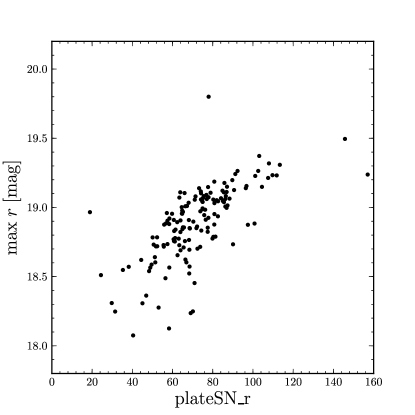
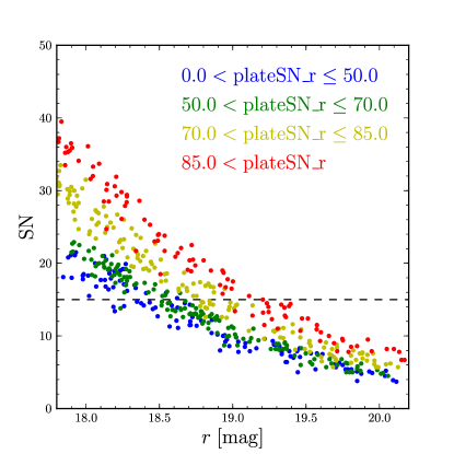
Figure 9.— Maximum apparent $r$-band magnitude per plate versus overall plate signal-to-noise ratio plateSN_r for the G-star sample with SN $>15$ for faint plates (top panel). Signal-to-noise ratio SN for stars on four typical SEGUE plates as a function of the apparent $r$-band magnitude (bottom panel). The four plates have been chosen to show a range in overall plate signal-to-noise ratio plateSN_r.

To infer the dependence on color and apparent magnitude of the selection function, we look at the distribution of the potential G-star targets in color–magnitude space. This is shown in Figure 8. The distribution of the spectroscopic sample is overlaid. This shows that the spectroscopic sampling is relatively fair in $g-r$ color, with some frayed edges because of changes between target and current photometry, and that the selection as a function of $r$-band magnitude tapers at the faint end, as should be expected when using a signal-to-noise ratio cut. If all SEGUE plates were integrated to the same depth, the signal-to-noise ratio cut should be a clean cut in $r$, but it is clear from Figure 8 that this is not the case. To distinguish between relatively shallow and relatively deep plates, we introduce the overall plate signal-to-noise ratio plateSN_r

$$\mathrm{plateSN\_r}=(\mathrm{sn1\_1}+\mathrm{sn2\_1})/2\,,$$ (A1)

where sn1_1 and sn2_1 are the $r$-band plate signal-to-noise ratio for the two SDSS spectrographs (see Table 17 in Stoughton et al., 2002). The faintest spectroscopic G-type star per plate as a function of plateSN_r for the faint plates is shown in Figure 9 for the faint plates. This figure shows that there is a clear difference in the faintest object that could have been successfully observed at $SN>15$ between relatively shallow and relatively deep plates. The bottom panel of Figure 9 shows the signal-to-noise ratio of stars on four plates chosen to cover a range in the overall plate signal-to-noise ratio. This shows that the $SN>15$ cut for the entire sample translates into a fairly sharp $r$-band cut for each individual plate.

Our model for the SEGUE G-star selection function is then the following: For each plate we find the faintest targeted object in $r$-band magnitude with SN larger than our signal-to-noise-ratio cut, with apparent magnitude $r_{\mathrm{cut}}$ (if this object is fainter than the nominal limit $r_{\mathrm{max}}$ for bright or faint plates, we set $r_{\mathrm{cut}}$ equal to this limit; $r_{\mathrm{max}}=17.8$ mag for bright plates and 20.2 mag for faint plates), and then assume that the selection function for that plate is given by a hyperbolic tangent cut-off, centered on $r_{\mathrm{cut}}-0.1$ mag, and with a width-parameter whose natural logarithm is -3 ($\approx 0.05$ mag), such that the total width of the cut-off is about 0.2 mag and the faintest object on the plate is about 2 widths from the center of the cut-off. The function value at the bright end is equal to the number of spectroscopic objects brighter than $r_{\mathrm{cut}}$ divided by the total number of targets brighter than $r_{\mathrm{cut}}$. Thus, the plate-dependent selection function is given by

$$\begin{split}S(\mathrm{plate},&r,g-r)=\\ &\frac{\#\mathrm{spectroscopic\ objects\ with}\ r_{\mathrm{min}}\leq r\leq r_{\mathrm{cut}}}{\#\mathrm{targets\ with}\ r_{\mathrm{min}}\leq r\leq r_{\mathrm{cut}}}\times\left[1-\tanh\left(\frac{r-r_{\mathrm{cut}}+0.1}{\exp\left(-3\right)}\right)\right]\Big{/}2\,,\end{split}$$ (A2)

where the numbers of objects are evaluated within the $\approx 7$ deg² area of the plate in question and in the $0.48\leq g-r\leq 0.55$ G-star color range; $r_{\mathrm{min}}$ is 14.5 mag for bright plates and 17.8 mag for faint plates. The selection function is zero outside of the apparent $r$-band magnitude range of the plate ($[14.5,17.8]$ for bright plates and $[17.8,20.2]$ for faint plates).

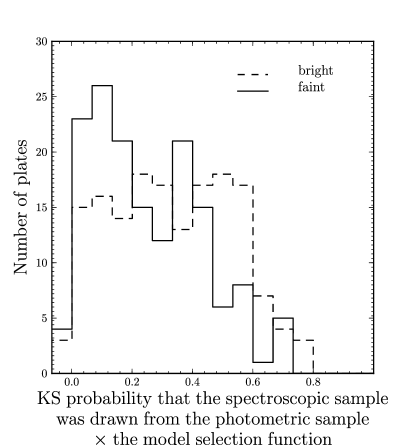
Figure 10.— Distribution of the probability that a plate’s spectroscopic sample was drawn from the photometric sample combined with the model selection function. The leftmost bin contains the plates with probability $<0.001$. For the correct model of the SEGUE selection function, the distribution should be approximately flat between zero and one.

We use this model both for the bright plates and the faint plates, although most bright plates are in fact consistent with being complete up to 17.8 mag. Figure 10 shows the distribution of Kolmogorov-Smirnov (KS) probabilities that the spectroscopic sample for any given plate was selected from the target sample with this model for the selection function. All but 7 plates have probabilities larger than 0.001 and the distribution of probabilities is relatively flat, as expected.

Rather than using a smooth hyperbolic tangent cut-off, we also tried a sharp cut at $r_{\mathrm{cut}}$. With this model for the selection function, 79 plates have a KS probability $<0.05$ ($\approx$25 percent of the number of plates), as opposed to 30 plates in the hyperbolic-tangent-cut-off model ($\approx$9 percent of the sample). Therefore, the smooth cut-off is necessary to fully model the selection function. The fact that the distribution of KS probabilities in Figure 10 is not entirely flat is due to remaining details in the faint cut-off of the selection function, as we know that the selection function is flat at brighter magnitudes. This does not impact our analsis greatly, as most stars are much brighter than the cut-off (as compared to the scale over which the selection function changes near the cut-off).

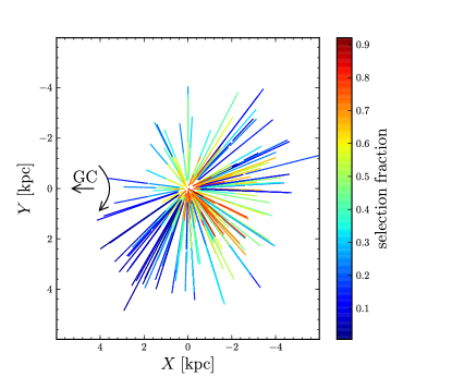
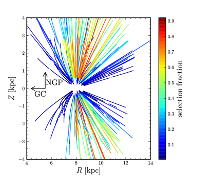
Figure 11.— The SEGUE selection function—the fraction of objects successfully observed spectroscopically with SN $>15$ —for the G-star sample, as a function of Galactic coordinates $X$ and $Y$ (left panel), and of Galactocentric radius $R$ and vertical height $Z$ (right panel). The $r$-dependent SEGUE selection function is here transformed into spatial coordinates using the photometric distance relation applied to a color $g-r=0.515$ mag and [Fe/H] = -0.5.

The selection function is simplest in its native coordinates, survey plate, and $r$-band magnitude. For each value of $g-r$ and [Fe/H], the $r$-dependent selection function above translates into a (different) spatial selection function through the use of the photometric distance relation. The selection function projected into spatial coordinates for a typical value of $g-r$ and [Fe/H] is shown in Figure 11. Near $|b|=90^{\circ}$ the spectroscopic sample is relatively complete, whereas near the Galactic plane the selection is much less complete.

We have posted Python code that implements this model for the SEGUE selection function. It is publicly available at

https://github.com/jobovy/segueSelect .

Appendix B The Magnitude–color–metallicity density and estimates of the effective survey volume

The density in magnitude–color–metallicity space needs to be included in the likelihood in equation (6), because it forms the basis of the photometric distance relation used to translate observed colors, metallicities, and apparent magnitudes into distances, which ultimately relate to the effective search volume. We assume here for simplicity that stars of a given $g-r$ and $[\mathrm{Fe/H}]$ follow a single stellar isochrone given by the Ivezić et al. (2008) photometric distance relation in terms of $g-r$ using equation (1) to translate $g-r$ into the $g-i$ color used by the Ivezić et al. (2008) relation. The reason for expressing the Ivezić et al. (2008) $g-i$–metallicity–magnitude relation into $g-r$ is to keep the integration in equation (7) simple; if we had chosen to use the $g-i$ relation we would have to include the $r-i$ color as well, and model and integrate over the full $g-r$,$r-i$ plane. As the stellar locus is very narrow ($\lesssim 0.1$ mag), this adds less (random) scatter than is intrinsic to the photometric distance relation.

In the single-isochrone model, $\rho(r,g-r,[\mathrm{Fe/H}]|R,Z,\phi)$ becomes the product of a delta function with the density in the color–metallicity plane

$$\rho(r,g-r,[\mathrm{Fe/H}]|R,Z,\phi)=\delta(r-r[g-r,[\mathrm{Fe/H}],d]|R,Z,\phi)\,\rho(g-r,[\mathrm{Fe/H}]|R,Z)\,,$$ (B1)

where $r[g-r,[\mathrm{Fe/H}],d]$ is the apparent magnitude derived from the photometric distance relation combined with the distance, and by a slight abuse of notation we have used the same symbol to denote the density in the color–metallicity plane. We assume that this density is independent of Galactocentric azimuth $\phi$, but for now allow it to depend on $R$ and $Z$. Using this, the normalization integral in equation (7) simplifies to

$$\begin{split}\int&\mathrm{d}l\,\mathrm{d}b\,\mathrm{d}d\,\mathrm{d}r\,\mathrm{d}(g-r)\,\mathrm{d}[\mathrm{Fe/H}]\,\lambda(l,b,d,r,g-r,[\mathrm{Fe/H}]|\theta)\\ &=A_{p}\,\sum_{\mathrm{plates}\ p}\int\mathrm{d}(g-r)\,\mathrm{d}[\mathrm{Fe/H}]\,\\ &\,\times\int_{d[r_{\mathrm{min}},g-r,[\mathrm{Fe/H}]]}^{d[r_{\mathrm{max}},g-r,[\mathrm{Fe/H}]]}\mathrm{d}d\,S(p,r[g-r,[\mathrm{Fe/H}],d],g-r)\,\rho(g-r,[\mathrm{Fe/H}]|R,Z)\,d^{2}\,\nu_{*}(R,z|l,b,d,\theta)\,,\end{split}$$ (B2)

where $r_{\mathrm{min}}$ and $r_{\mathrm{max}}$ are the minimum and maximum apparent magnitude of plate $p$, and the functions $d[\cdot]$ and $r[\cdot]$ use the photometric distance relation.

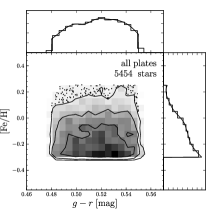
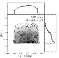
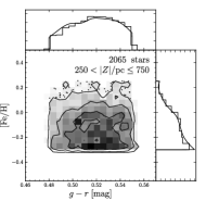
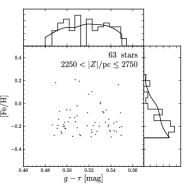
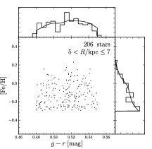
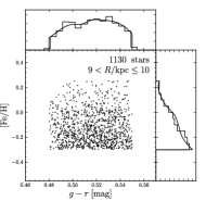
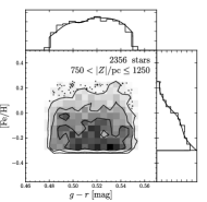
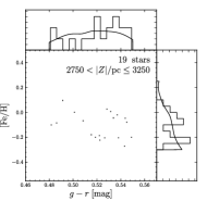
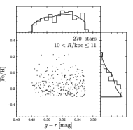
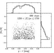
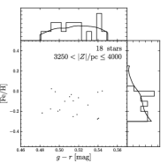
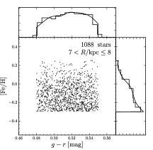
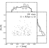
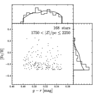
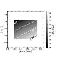
Figure 12.— Distribution of [Fe/H] and $g-r$ for the full $\alpha$-young G-dwarf sample (top, left panel) and split into ranges in Galactocentric radius $R$ and vertical height $|Z|$ (other panels). Linear binned densities with contours containing 68, 95, and 99 percent of the distribution and individual outliers beyond 99 percent are shown in spatial bins with more than 1,500 stars. A smooth interpolation of the one-dimensional distributions in the top left panel is shown in all panels. The bottom right panel shows the absolute $r$-band magnitude as a function of $g-r$ and [Fe/H] from the Ivezić et al. (2008) color–metallicity–magnitude relation (their eqn. A7).

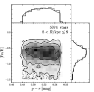
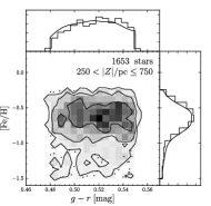
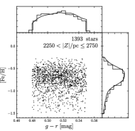
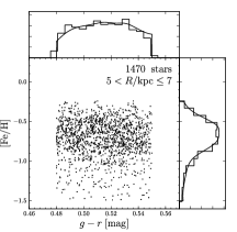
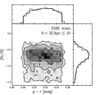
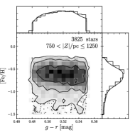
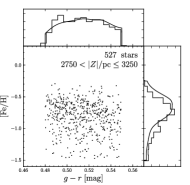
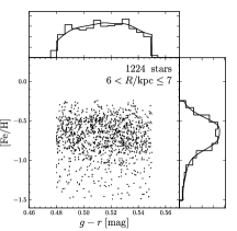
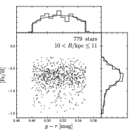
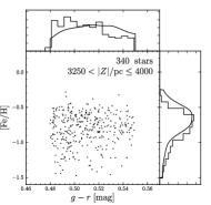
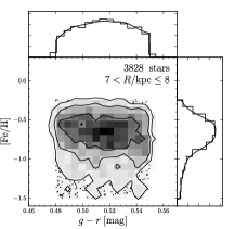
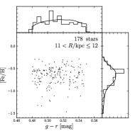
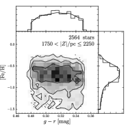
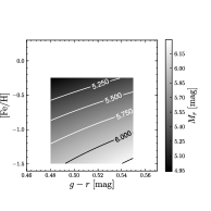
Figure 13.— Same as Figure 12, but for the $\alpha$-old G-dwarf sample.

The color–metallicity distribution for the $\alpha$-young and $\alpha$-old sample is shown in Figures 12 and 13, respectively. The top-left panel shows the distribution for the entire sample; the remaining panels show the color–metallicity distribution as a function of Galactocentric radius (including all vertical heights) and as a function of vertical height (including all Galactocentric radii). For both samples, the color–metallicity distribution separates into the product of one-dimensional color and metallicity distributions, thus we assume that $\rho(g-r,[\mathrm{Fe/H}]|R,Z)=\rho^{c}(g-r|R,Z)\,\rho^{[\mathrm{Fe/H}]}([\mathrm{Fe/H}]|R,Z)$. The $g-r$ distribution is independent of $R$ and $Z$ for both the $\alpha$-young and the $\alpha$-old sample; we use a spline interpolation of the color distribution for the full sample for $\rho^{c}(g-r|R,Z)$, independent of $R$ and $Z$. This interpolation is shown in the top histogram in all panels of Figures 12 and 13. The metallicity distribution of the $\alpha$-old sample is also mostly independent of $R$ and $Z$, with only a hint of a trend toward a more metal-poor distribution at large distances from the plane. The $[\mathrm{Fe/H}]$ distribution of the $\alpha$-young sample shows expected trends with $R$ and $Z$: The peak of the metallicity distribution goes from more metal-rich closer to the Galactic center and closer to the plane, to more metal-poor at larger Galactocentric radii and at larger $Z$. These shifts are modest ($\lesssim 0.1$ dex), which is partly due to the fact that farther from the Solar radius we preferentially see stars at larger distances from the plane. We stress that these metallicity distributions are the observed distributions uncorrected for selection effects, but selection effects play a minor role and merely shift the overall distribution by $\approx$ 0.1 dex (Schlesinger et al., 2011, in preparation). We investigate the effect of systematically shifting the metallicity distribution below.

The effect of metallicity and color on the absolute magnitude using the Ivezić et al. (2008) color–metallicity–magnitude relation is shown in the bottom right panel of Figures 12 and 13, for the ranges in color and metallicity considered for both samples. From the blue and metal-rich to the red and metal-poor end the shift in absolute magnitude is about 1 mag, or a factor of about 1.6 in distance.

As the $\alpha$-old metallicity distribution depends only weakly on $R$ and $Z$, we will assume that it is constant, and use a spline interpolation of the $[\mathrm{Fe/H}]$ distribution of the full sample as our model for $\rho^{[\mathrm{Fe/H}]}([\mathrm{Fe/H}]|R,Z)$. We do the same for the $\alpha$-young sample, even though there are slight trends with $R$ and $Z$. These models are shown in the right histograms of all panels in Figures 12 and 13. We can then simplify the normalization integral in equation (B2) further to

$$\begin{split}\int&\mathrm{d}l\,\mathrm{d}b\,\mathrm{d}r\,\mathrm{d}d\,\mathrm{d}r\,\mathrm{d}(g-r)\,\mathrm{d}[\mathrm{Fe/H}]\,\lambda(l,b,d,r,g-r,[\mathrm{Fe/H}]|\theta)\\ &=A_{p}\,\sum_{\mathrm{plates}\ p}\int\mathrm{d}(g-r)\,\rho^{c}(g-r|R,Z)\int\mathrm{d}[\mathrm{Fe/H}]\,\rho^{[\mathrm{Fe/H}]}([\mathrm{Fe/H}]|R,Z)\\ &\,\times\int_{d[r_{\mathrm{min}},g-r,[\mathrm{Fe/H}]]}^{d[r_{\mathrm{max}},g-r,[\mathrm{Fe/H}]]}\mathrm{d}d\,S(p,r[g-r,[\mathrm{Fe/H}],d],g-r)\,d^{2}\,\nu_{*}(R,z|l,b,d,\theta)\,.\end{split}$$ (B3)

If we then determine the overall minimum and maximum heliocentric distance at which we can observe stars in both samples, we can calculate the inner integral between these limits, with the understanding that the selection function is zero outside of the apparent-magnitude range of the plate in question (since bluer or more metal-rich stars can only be observed at distances starting at a value that is larger than the overall minimum distance, and redder and more metal-poor stars can only be seen out to distances that fall short of the overall maximum distance, because of the color and metallicity dependence of the photometric distance method). We can then calculate the integral by summation on a regular grid as

$$\begin{split}\int&\mathrm{d}l\,\mathrm{d}b\,\mathrm{d}r\,\mathrm{d}d\,\mathrm{d}(g-r)\,\mathrm{d}[\mathrm{Fe/H}]\,\lambda(l,b,d,r,g-r,[\mathrm{Fe/H}]|\theta)\\ &=A_{p}\,\sum_{\mathrm{plates}\ p}\sum_{d}\,d^{2}\,\nu_{*}(R,z|l,b,d,\theta)\,\\ &\qquad\sum_{g-r}\,\sum_{[\mathrm{Fe/H}]}\,\rho^{c}(g-r)\,\rho^{[\mathrm{Fe/H}]}([\mathrm{Fe/H}])\,S(p,r[g-r,[\mathrm{Fe/H}],d],g-r)\,,\end{split}$$ (B4)

where the distance summation is between the overall minimum and maximum distance. We dropped integration factors $\Delta d$, $\Delta(g-r)$, and $\Delta[\mathrm{Fe/H}]$, as these only contribute terms that do not depend on the parameters $\theta$ in the log likelihood in equation (8) (note that they do contribute when we do not marginalize over the amplitude of the density in equation [6]). Written in this way, this normalization integral can be computed efficiently, as all of the necessary coordinate transformations, selection function evaluations, and color–metallicity-distribution function calls can be pre-computed on a dense grid.

Appendix C Detailed data versus model comparisons

In this Appendix we present detailed comparisons of our best-fit density models with the observed data, as ultimately the best-fit density parameters are constrained through the quality of the fit in the natural coordinates of the spectroscopic data ($l,b,r,g-r,[\mathrm{Fe/H}]$). We also show that the results we obtain for different sub-samples of our nominal samples are consistent with the best fits for the full samples. As we fit density models by forward modeling the underlying density model, i.e., by taking the spatial density and running it through the SEGUE selection function and the photometric distance relation, we cannot show direct maps of the density in any meaningful way without massaging the data excessively. Therefore, we compare the observed star counts with the best-fit model by running the underlying star counts model through the selection function and photometric magnitude–color–metallicity relation, and then comparing it with the observed star counts. This has the added advantage that it shows that the entire framework of (a) the underlying density, (b) the photometric magnitude–color–metallicity relation, and (c) our model of the SEGUE selection function provides a valid description of the observed data.

C.1. The $\alpha$-old disk stars

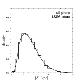
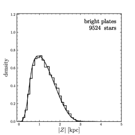
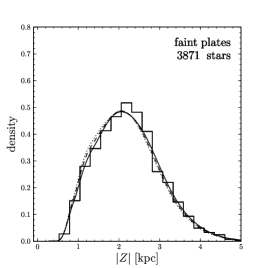
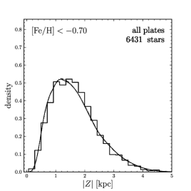
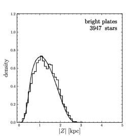
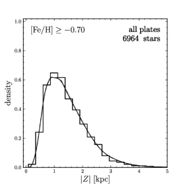
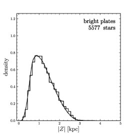
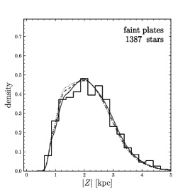
Figure 14.— Comparison between the observed distribution of vertical heights of the $\alpha$-old G-dwarf sample and the distribution predicted by the best-fit mixture of two double-exponential disks. The dashed and dotted lines show the same model, but with a scale length of 3 and 4 kpc, respectively. The bottom two rows show the nominal sample used in the top row split at $[\mathrm{Fe/H}]$ = $-0.7$. See Table 2 for the parameters of the best-fit models.

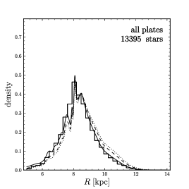
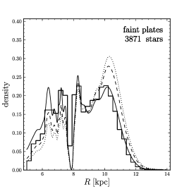
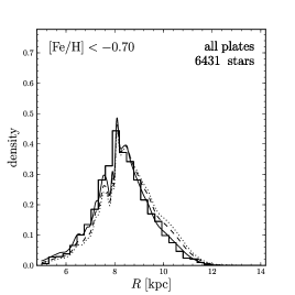
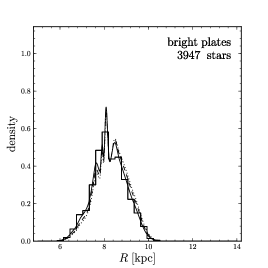
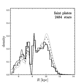
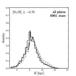
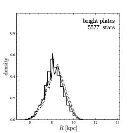
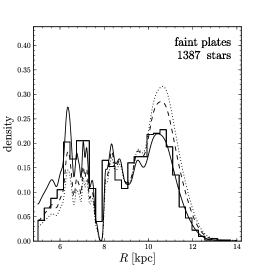
Figure 15.— Same as Figure 14, but for the distribution of Galactocentric radii. The dashed and dotted lines show the same model but with a scale length of 3 and 4 kpc, respectively.

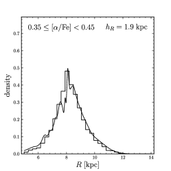
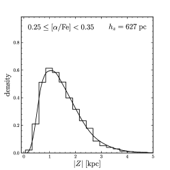
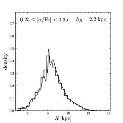
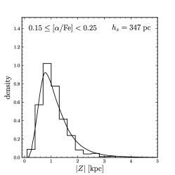
Figure 16.— Structural parameters of the G-dwarf sample as a function of $[\alpha\mathrm{/Fe}]$. The top two rows show the $\alpha$-old sample split at $[\alpha\mathrm{/Fe}]$ = 0.35; the bottom two rows contain the $\alpha$-young sample split at $[\alpha\mathrm{/Fe}]$ = 0.15. The left column compares the observed distribution of vertical heights to the model distribution. The right column does the same for the distribution of Galactocentric radii. Each sample is fit with a mixture of two double-exponential disks. The best-fit parameters of the dominant disk component are shown in the top-left of each panel. In each case the secondary component only contributes a few percent of the mass at the solar circle (see Tables 2 and 4 for detailed results).

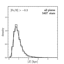
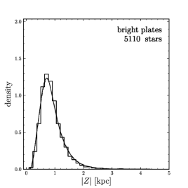
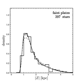
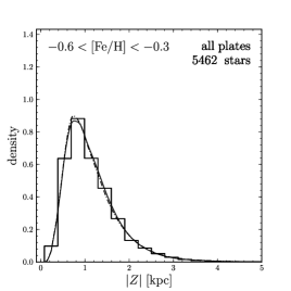
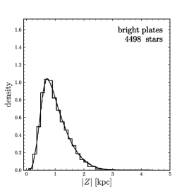
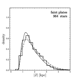
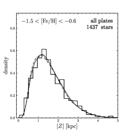
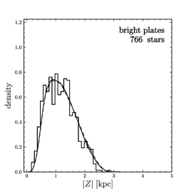
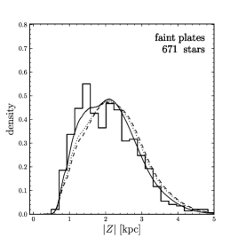
Figure 17.— Comparison between the observed distribution of vertical heights of the $\alpha$-young G-dwarf sample and the distribution predicted by the best-fit mixture of two double-exponential disks model. The dashed and dotted lines show the same model, but with a scale length of 2 and 3 kpc, respectively. The bottom two rows show samples with the same $[\alpha\mathrm{/Fe}]$ range of the nominal $\alpha$-young sample, but with different $[\mathrm{Fe/H}]$ boundaries. See Table 4 for the parameters of the best-fit models.

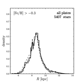
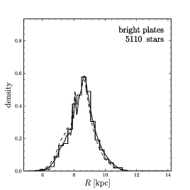
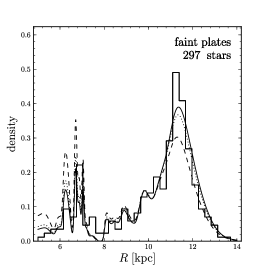
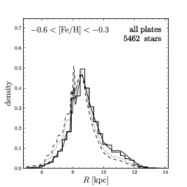
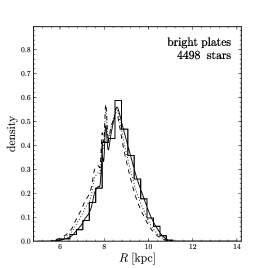
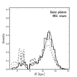
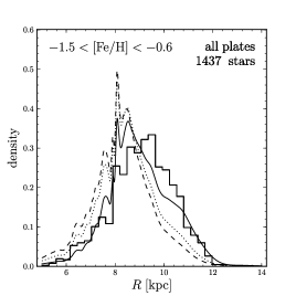
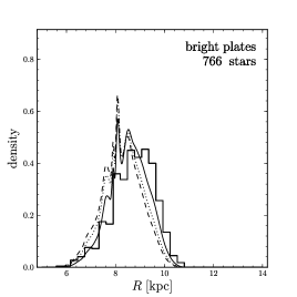
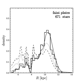
Figure 18.— Same as Figure 17, but for the distribution of Galactocentric radii. The dashed and dotted lines show the same model, but with a scale length of 2 and 3 kpc, respectively.

Figure 14 compares the observed distribution of vertical heights $|Z|$ of the $\alpha$-old G-dwarf sample to that predicted by the best-fit model. This prediction is obtained by running the best-fit density model integrated over the color–metallicity distribution through our model for the SEGUE selection function. There are 35 stars with magnitudes that should put them on faint plates, but that were observed on bright plates, and 551 stars in the opposite situation are cut from the data sample to show this comparison. The comparison between the data and the model is shown for all plates and for the bright and faint plates separately. The agreement between the model and observed distribution is excellent for all of these. Figure 15 shows a similar comparison for the distribution of Galactocentric radii of the data and in the model. The model correctly predicts the observed star counts for most Galactocentric radii, except the smallest around 5 kpc, where the model slightly overpredicts the number of stars (here, and in further comparisons below, the model around 8 kpc behaves somewhat erratically, as this is the boundary between $90^{\circ}\leq l\leq 270^{\circ}$ and $-90^{\circ}<l<90^{\circ}$ plates, and we do not use the finite extent of the plate in our model distributions). Also shown in this figure and in Figure 14 are models that only differ from the best-fit model in their radial scale length: a model with a scale length of 3 kpc and one with a scale length of 4 kpc. It is clear that these longer scale lengths are strongly ruled out by the model, as they strongly overpredict the star counts at large Galactocentric radii.

Table 2 lists the best-fit parameters for fits that only use (a) bright or faint plates, (b) $b>0^{\circ}$ or $b<0^{\circ}$ plates, or (c) $|b|>45^{\circ}$ or $|b|<45^{\circ}$ plates. The results from all of these different samples are roughly consistent with each other; we note that we can even measure the radial scale length with high-latitude plates ($|b|>45^{\circ}$) alone.

Figures 14 and 15 show comparisons between the observed star counts and the model, when we split the $\alpha$-old sample into more metal-poor and more metal-rich sub-samples by cutting the sample at [Fe/H] = $-0.7$. Comparisons for when we split the $\alpha$-old sample into two bins in $[\alpha\mathrm{/Fe}]$, by cutting the sample at $[\alpha\mathrm{/Fe}]$ = 0.35, are shown in Figure 16.

C.2. The $\alpha$-young disk sample

Figure 17 compares the best-fit model to the observed star counts as a function of vertical height and Figure 18 shows this comparison as a function of Galactocentric radius, again removing 4 stars with magnitudes that should put them on faint plates but that were observed on bright plates and removing 43 stars in the opposite situation. We also show models whose parameters are the same as those of the best-fit model, but with shorter scale lengths of 2 and 3 kpc. The faint plates, which only contain 6 percent of the $\alpha$-young sample, rule out a short scale length of 2 kpc for the $\alpha$-young disk. The best-fit model provides a good fit to the observed star counts.

We again also list the best-fit parameters for fits that only use (a) bright or faint plates, (b) $b>0^{\circ}$ or $b<0^{\circ}$ plates, or (c) $|b|>45^{\circ}$ or $|b|<45^{\circ}$ plates in Table 4. The results from all of these different samples are again roughly consistent, except for the faint plates fit, which prefer even longer radial scale lengths, but faint plates only contain 6 percent of the $\alpha$-young sample. We have also run fits for the $\alpha$-young sample where we (a) employ a more conservative SN cut of $SN>30$, (b) enlarge our sample with a less conservative SN cut of $SN>10$, (c) remove stars on plates whose K-S probability for the spectroscopic sample to have been drawn from the underlying photometric sample combined with our model for the SEGUE selection function (see Figure 10) is smaller than 0.1, (d) use stars from the SEGUE database that were explicitly targeted as G-type stars (with all other log g, SN, $E(B-V)$ cuts), (e) remove stars with magnitudes that should put them on SEGUE bright plates, but that were observed as part of a faint plate and vice versa, and (f) artificially shift the metallicity distribution 0.1 dex toward the more metal-rich end. The results from these fits are all consistent with those obtained for our nominal sample with fiducial cuts.

Figures 17 and 18 show comparisons between the observed and predicted star counts for the $\alpha$-young samples that are more metal-poor than the nominal $\alpha$-young sample. The fit for the $-0.6<$ $[\mathrm{Fe/H}]$ $<-0.3$ sample is good, while the fit for the most metal-poor $\alpha$-young sub-sample is not entirely satisfactory. Comparisons between the observed star counts and the model when we split the $\alpha$-young sample into two, by cutting at $[\alpha\mathrm{/Fe}]$ = 0.15, are shown in the lower two rows of Figure 16.

Appendix D Analysis test on mock data samples

Figure 19.— *

Analysis of mock data assuming thin–thick disk dichotomy

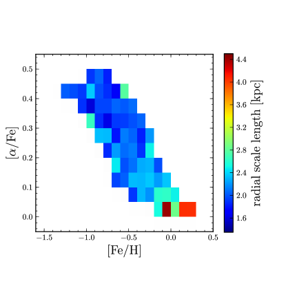
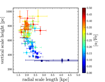
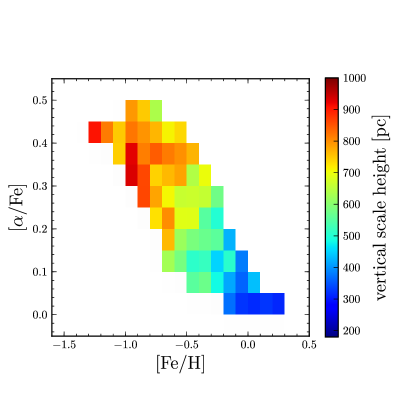
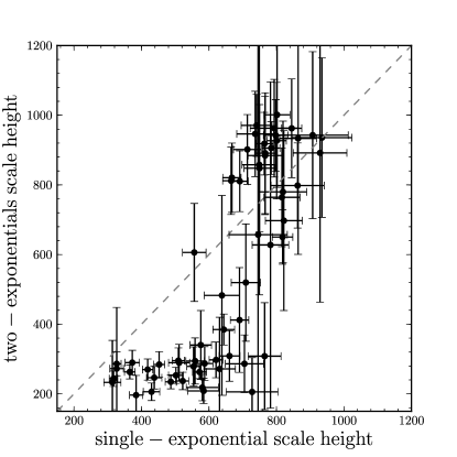
Figure 20.— Results from applying this paper’s analysis to a mock data sample composed of a two-component thin–thick disk sample. Assuming abundance errors of 0.2 dex in $[\mathrm{Fe/H}]$ and 0.15 in $[\alpha\mathrm{/Fe}]$, we deconvolve the observed distribution in ($[\mathrm{Fe/H}]$,$[\alpha\mathrm{/Fe}]$) (Figure 2) into two Gaussian components, which are assumed to correspond to a thin component ($h_{z}$ = 300 pc, $h_{R}$ = 3.5 kpc) and a thick component ($h_{z}$ = 850 pc, $h_{R}$ = 2 kpc). The panels on the left show the results of fitting single-exponential models in each mono-abundance bin, as in Figure 4. The top panel on the right shows the single-exponential scale height vs. scale length color-coded by $[\alpha\mathrm{/Fe}]$. The bottom right panel shows the scale height of the dominant component when fitting a mixture of two expontial components vs. the single-exponential scale height. In contrast to the fits for the real data sample, this latter plot shows that the mixture-model is preferred and thus we confidently infer that in the mock-data sample each bin is made up of two populations (at least for those with single-exponential $h_{z}\lesssim 800$ pc). Other differences with the real data are that most mono-abundance bins have a short single-exponential scale length due to the contamination from the short, thick disk component and, similarly, that the single-exponential scale heights quickly reach “thick” values of $h_{z}\gtrsim 600$ pc when going to more metal-poor and $[\alpha\mathrm{/Fe}]$-enhanced populations. We conclude that abundance errors cannot turn a clearly thin–thick separated disk sample into the results we observe for the real data set in Figures 4 to 6.

In order to test the methodology for fitting the density discussed in $\mathsection$ 3, and as check on the code, we create mock data samples selected in exactly the same way as the SEGUE G-dwarf sample and fit them using our algorithm. We also use this framework to test whether the results we obtain can plausibly be the result of abundance errors smoothing out an underlying two-component thin–thick disk structure.

We create mock data sampled from a model underlying density by calculating, for each line of sight, (i) the fraction of stars in the sample that lies along that line of sight and (ii) the distribution in $r$-band magnitude as a function of color $g-r$ and metallicity $[\mathrm{Fe/H}]$. For calculating both of these, we take the SEGUE selection function, described in Appendix A, into account. Thus, we can obtain a sample that is equivalent to what SEGUE would have observed for a particular density model.

To test the methodology and code we populate each mono-abundance bin in the ($[\mathrm{Fe/H}]$,$[\alpha\mathrm{/Fe}]$) plane with a sample drawn from a thin-disk component with $h_{z}=300$ pc and $h_{R}=3.5$ kpc, keeping the abundances and number of stars in each bin the same as in the observed sample. We then run the same analysis code on this sample as is run to produce the real data results in Figures 4 to Figures 6. We find results that are consistent with the input model within the uncertainties for each bin. The uncertainties are similar to those found for the real data near $h_{z}=300$ pc and $h_{R}=3.5$ kpc. We repeat this for an input “thick” disk model with $h_{z}=850$ pc and $h_{R}=2$ kpc, and again find results that are consistent with the input model within the uncertainties.

We use a similar procedure to investigate whether abundance errors can smooth out an underlying disk model made up of a thin- and thick-disk component without showing up in our analysis. Assuming SEGUE abundance uncertainties of 0.2 dex in $[\mathrm{Fe/H}]$ and 0.15 dex in $[\alpha\mathrm{/Fe}]$, we first model the underlying abundance distribution using two Gaussian components, and fit this model to the observed distribution with the assumed abundance uncertainties using the extreme-deconvolution technique (Bovy et al., 2011). We use a Gaussian mixture model for the underlying distribution solely as a convenient of decomposing the observed distribution for the purpose of this test. The two-Gaussian mixture model adequately represents the observed distribution after convolving again with the uncertainties. The best-fit mixture has a Gaussian centered near solar abundances (40 percent of the sample; $[\mathrm{Fe/H}]$ = $-0.3$ dex, $[\alpha\mathrm{/Fe}]$ = 0.1 dex) and one at metal-poor and $\alpha$-enhanced abundances (60 percent of the sample; $[\mathrm{Fe/H}]$ = $-0.7$ dex, $[\alpha\mathrm{/Fe}]$ = 0.35 dex). To reproduce the observed distribution, these components both need a dispersion of 0.2 dex in $[\mathrm{Fe/H}]$ and 0.07 dex in $[\alpha\mathrm{/Fe}]$, with a correlation of $-0.85$ and $-0.6$, respectively. We then assign stars to these two components with probabilities computed from their posterior probability of being drawn from either component, based on their abundances and assumed abundance uncertainties. We sample new $r$-band magnitudes and coordinates for these stars based on the component they are assigned to: we draw the stars assigned to the solar-abundances component from a thin-disk density with $h_{z}$ = 300 pc and $h_{R}=3.5$ kpc, and stars assigned to the $\alpha$-enhanced component from a thick-disk distribution with $h_{z}=850$ pc and $h_{R}$ = 2.5 kpc. We then run the same analysis code on this sample as is run on the real data.

The results from this test are shown in Figure 20. Although in certain respects they are similar to the results for the real data, they are different in a few crucial ways. Most importantly, when fitting a mixture of two exponential models to each bin we find unambiguous evidence in many bins for two components. This is shown in the lower right panel of Figure 20, where the scale height of the dominant component when fitting the mixture is shown vs. the scale height when fitting a single exponential. For most bins with single-exponential $h_{z}\lesssim 800$ pc, the dominant component is the $h_{z}=300$ pc input thin-disk component. Therefore, even though the abundance pattern of the single-exponential scale height in the lower left panel of Figure 20 is smooth between thin and thick components, most bins are actually resolved into the two input components. This is a major difference with the real data, for which the equivalent comparison, shown in Figure 6, shows a striking one-to-one correlation between the single-exponential and the mixture scale height, with no evidence for a second component for the vast majority of the mono-abundance bins.

In addition to the fact that our analysis correctly identifies two components in each mono-abundance bin in the mock data, the abundance dependence of the inferred single-exponential scale height and scale length is also quite different from that of the mock data. The inferred scale length for the mock data is short for most abundance bins and only reaches $h_{R}\gtrsim 3$ kpc for those abundance bins that are farthest from the center of the metal-poor and $\alpha$-enhanced abundance component. Thus, the contamination from the thick-disk component with its short scale length drives the inferred scale length for most abundance bins to small values. This behavior is not observed in the real data (Figure 4). The abundance dependence of the single-exponential scale height for the mock data is also much steeper than observed in the real data, with values of $h_{z}\gtrsim 600$ pc as metal-rich as $[\mathrm{Fe/H}]$ = -0.3.

From these tests we conclude that abundance errors cannot explain the single-exponential components we observe in each mono-abundance bin in the real data or the abundance behavior of the scale height and scale length. Based on an entirely different argument that uses the observed isothermality of the vertical kinematics of the same mono-abundance populations, Bovy et al. (2012b) infer that the internal SEGUE abundance uncertainties are likely somewhat smaller than the values reported by SEGUE, with likely uncertainties of 0.15 dex in $[\mathrm{Fe/H}]$ and 0.07 dex in $[\alpha\mathrm{/Fe}]$. Thus, abundance uncertainties do not influence the main conclusions of this paper.

References

- Abadi et al. (2003) Abadi, M. G., Navarro, J. F., Steinmetz, M., & Eke, V. R. 2003, ApJ, 591, 499
- Abazajian et al. (2009) Abazajian, K. N., Adelman-McCarthy, J. K., Agũeros, M. A., et al. 2009, ApJS, 182, 543
- Abt & Levy (1976) Abt, H. A. & Levy, S. G. 1976, ApJS, 30, 273
- Allende Prieto et al. (2008) Allende Prieto, C., Sivarani, T., Beers, T. C., et al. 2008, AJ, 136, 2070
- An et al. (2009) An, D., Pinsonneault, M. H., Masseron, T., et al. 2009, ApJ, 700, 523
- Aumer & Binney (2009) Aumer, M. &Binney, J. J. 2009, MNRAS, 397, 1286
- Bate et al. (2003) Bate, M. R., Bonnell, I. A., & Bromm, V. 2003, MNRAS, 339, 577
- Bate (2005) Bate, M. R. 2005, MNRAS, 363, 363
- Bell et al. (2008) Bell, E. F., Zucker, D. B., Belokurov, V., et al. 2008, ApJ, 680, 295
- Bensby et al. (2003) Bensby, T., Feltzing, S., & Lundström, I. 2003, A&A, 410, 527
- Bensby et al. (2005) Bensby, T., Feltzing, S., Lundström, I., & Ilyin, I. 2005, A&A, 433, 185
- Bensby et al. (2011) Bensby, T., Alves-Brito, A., Oey, M. S., Yong, D., & Meléndez, J. 2011, ApJ, 735, L46
- Bird et al. (2011) Bird, J. C., Kazantzidis, S., & Weinberg, D. H. 2011, MNRAS, submitted, arXiv:1104.0933
- Blanton et al. (2003) Blanton, M. R., Lupton, R. H., Miller Malley, F., et al. 2003, AJ, 125, 2276
- Bournaud et al. (2009) Bournaud, F., Elmegreen, B. G., & Martig, M. 2009, ApJ, 707, L1
- Bovy et al. (2009a) Bovy, J., Hogg, D. W., & Roweis, S. T. 2009a, ApJ, 700, 1794
- Bovy et al. (2009b) Bovy, J., Hogg, D. W., & Rix, H.-W. 2009b, ApJ, 704, 1704
- Bovy & Hogg (2010) Bovy, J. & Hogg, D. W. 2010, ApJ, 717, 617
- Bovy et al. (2011) Bovy, J., Hogg, D. W., & Roweis, S. T. 2011, Ann. Appl. Stat., 5, 1657, arXiv:0905.2979
- Bovy et al. (2012a) Bovy, J., Rix, H.-W., & Hogg, D. W. 2012a, ApJ, 751, 131
- Bovy et al. (2012b) Bovy, J., Rix, H.-W., Hogg, D. W., et al. 2012b, ApJ, submitted, arXiv:1202.2819
- Brook et al. (2004) Brook, C. B., Kawata, D., Gibson, B. K., & Freeman, K. C. 2004, ApJ, 612, 894
- Burstein (1979) Burstein, D. 1979, ApJ, 234, 829
- Buser et al. (1999) Buser, R., Rong, J., & Karaali, S. 1999, A&A, 348, 98
- Carlberg & Sellwood (1985) Carlberg, R. G., & Sellwood, J. A. 1985, ApJ, 292, 79
- Carollo et al. (2010) Carollo, D., Beers, T. C., Chiba, M., et al. 2010, ApJ, 712, 692
- Chen et al. (2001) Chen, B., Stoughton, C., Smith, J. A., et al. 2001, ApJ, 553, 184
- Cheng et al. (2011) Cheng, J., Rockosi, C. M., Morrison, H. L., et al. 2011, ApJ, submitted
- Chiba & Beers (2000) Chiba, M. & Beers, T. C. 2000, AJ, 119, 2843
- Dahlen et al. (2008) Dahlen, T., Strolger, L.-G., & Riess, A. G. 2008, ApJ, 681, 462
- Dalcanton et al. (1997) Dalcanton, J. J., Spergel, D. N., & Summers, F. J. 1997, ApJ, 482, 659
- Dehnen (1998) Dehnen, W. 1998, AJ, 115, 2384
- de Jong et al. (2007) de Jong, R. S., Seth, A. C., Radburn-Smith, D. J., 2007, ApJ, 667, 49
- De Simone, Wu, & Tremaine (2004) De Simone, R., Wu, X., & Tremaine, S. 2004, MNRAS, 350, 627
- Dierickx et al. (2010) Dierickx, M., Klement, R., Rix, H.-W., & Liu, C. 2010, ApJ, 725, L186
- Duquennoy & Mayor (1991) Duquennoy, A. & Mayor, M. 1991, A&A, 248, 485
- Fall & Efstathiou (1980) Fall, S. M. & Efstathiou, G. 1980, MNRAS, 193, 189
- Feltzing et al. (2003) Feltzing, S., Bensby, T., & Lundström, I. 2003, A&A, 397, 1
- Fischer & Marcy (1992) Fischer, D. A. & Marcy, G. W. 1992, ApJ, 396, 178
- Förster Schreiber et al. (2009) Förster Schreiber, N. M., Genzel, R., Bouché, N., et al. 2009, ApJ, 706, 1364
- Foyle et al. (2011) Foyle, K., Rix, H.-W., Dobbs, C. L., Leroy, A. K., & Walter, F. 2011, ApJ, 735, 101
- Fuhrmann (1998) Fuhrmann, K. 1998, A&A, 338, 161
- Fuhrmann (2008) Fuhrmann, K. 2008, MNRAS, 384, 173
- Fuhrmann (2011) Fuhrmann, K. 2011, MNRAS, 414, 2893
- Fukugita et al. (1996) Fukugita, M., Ichikawa, T., Gunn, J. E., Doi, M., Shimasaku, K., & Schneider, D. P. 1996, AJ, 111, 1748
- Gilmore & Reid (1983) Gilmore, G. & Reid, N. 1983, MNRAS, 202, 1025
- Gilmore & Wyse (1991) Gilmore, G. & Wyse, R. F. G. 1991, ApJ, 367, 55
- Gilmore et al. (2002) Gilmore, G., Wyse, R. F. G., & Norris, J. E. 2002, ApJ, 574, 39
- Goodman & Weare (2010) Goodman, J. & Weare, J. 2010, Comm. App. Math. and Comp. Sci., 5, 65
- Gott & Thuan (1976) Gott, J. R. & Thuan, T. X. 1976, ApJ, 204, 649
- Guedes et al. (2011) Guedes, J., Callegari, S., Madau, P., & Mayer, L. 2011, ApJ, 742, 76
- Gunn (1982) Gunn, J. E. 1982, in Astrophysical Cosmology, eds. H. A. Bruck, G. V. Coyne, & M. S. Longair (Pontificia Academia Scientarum)
- Gunn et al. (1998) Gunn, J. E., Carr, M., Rockosi, C., et al. 1998, AJ, 116, 3040
- Gunn et al. (2006) Gunn, J. E., Siegmund, W. A., Mannery, E. J., et al. 2006, AJ, 131, 2332
- Haywood (2008) Haywood, M. 2008, MNRAS, 388, 1175
- Hogg et al. (2001) Hogg, D. W., Finkbeiner, D. P., Schlegel, D. J., & Gunn, J. E. 2001, AJ, 122, 2129
- Ivezić et al. (2004) Ivezić, Ž., Lupton, R. H., Schlegel, D., et al. 2004, AN, 325, 583
- Ivezić et al. (2008) Ivezić, Ž., Sesar, B.; Jurić, M., et al. 2008, 684, 287
- Jurić et al. (2008) Jurić, M., Ivezić, Ž., Brooks, A., et al. 2008, 673, 864
- Katz & Gunn (1991) Katz, N. & Gunn, J. E. 1991, ApJ, 377, 365
- Kazantzidis et al. (2008) Kazantzidis, S., Bullock, J. S., Zentner, A. R., Kravtsov, A. V., Moustakas, L. A. 2008, apj, 688, 254
- van der Kruit & Searle (1981) van der Kruit, P. C. & Searle, L. 1981, A&A, 95, 105
- Lake & Carlberg (1988) Lake, G. & Carlberg, R. G. 1988, AJ, 96, 1581
- Larsen & Humphreys (2003) Larsen, J. A. & Humphreys, R. M. 2003, AJ, 125, 1958
- Larson (1976) Larson, R. B. 1976, MNRAS, 176, 31
- Lee et al. (2008a) Lee, Y. S., Beers, T. C., Sivarani, T., et al. 2008a, AJ, 136, 2022
- Lee et al. (2008b) Lee, Y. S., Bers, T. C., Sivarani, T., et al. 2008b, AJ, 136, 2050
- Lee et al. (2011a) Lee, Y. S., Beers, T. C., Allende Prieto, C., et al. 2011a, AJ, 141, 90
- Lee et al. (2011b) Lee, Y. S., Beers, T. C., An, D., et al. 2011b, ApJ, 738, 187
- Loebman et al. (2011) Loebman, S. R., Roškar, R., Debattista, V. P., et al. 2011, ApJ, 737, 8
- Lupton et al. (2001) Lupton, R., Gunn, J. E., Ivezić, Ž., et al. 2001, ASPC, 238, 269
- Machida et al. (2009) Machida, M. N., Omukai, K., Matsumoto, T., & Inutsuka, S. 2009, MNRAS, 399, 1225
- Majewski (1993) Majewski, S. R. 1993, ARA&A, 31, 575
- Malmquist (1920) Malmquist, K. G. 1920, Medd. Lunds Astron. Obs., Ser. 2., No. 22
- Malmquist (1922) Malmquist, K. G. 1922, Medd. Lunds Astron. Obs., Ser. 1, No. 100
- Maoz et al. (2011) Maoz, D., Mannucci, F., Li, W., et al. 2011, MNRAS, 412, 1508
- Matteucci & Recchi (2001) Matteucci, F. & Recchi, S. 2001, ApJ, 558, 351
- Meidt et al. (2009) Meidt, S. E., Rand, R. J., & Merrifield, M. R. 2009, ApJ, 702, 277
- Minchev & Famaey (2010) Minchev, I. & Famaey, B. 2010, ApJ, 722, 112
- Minchev et al. (2011) Minchev, I., Famaey, B., Combes, F., et al. 2010, A&A, 527, 147
- Mishenina et al. (2004) Mishenina, T. V., Soubiran, C., Kovtyukh, V. V., & Korotin, S. A. 2004, A&A, 418, 551
- Moster et al. (2010) Moster, B. P., Macciò, A. V., Somerville, R. S., Johansson, P. H., & Naab, T. 2010, MNRAS, 403, 1009
- Navarro et al. (2011) Navarro, J. F., Abadi, M. G., Venn, K. A., Freeman, K. C., & Anguiano, B. 2011, MNRAS, 412, 1203
- Neeser et al. (2002) Neeser, M. J., Sackett, P. D., De Marchi, G., & Paresce, F. 2002, A&A, 383, 472
- Norris (1987) Norris, J. 1987, ApJ, 314, L39
- Ojha (2001) Ojha, D. K. 2001, MNRAS, 322, 426
- Padmanabhan et al. (2008) Padmanabhan, N., Schlegel, D. J., Finkbeiner, D. P., et al. 2008, ApJ, 674, 1217
- Pier et al. (2003) Pier, J. R., Munn, J. A., Hindsley, R. B., et al. 2003, AJ, 125, 1559
- Pohlen et al. (2007) Pohlen, M., Zaroubi, S., Peletier, R. F., & Dettmar, R.-J. 2007, MNRAS, 378, 594
- Press et al. (2007) Press, W. H., Teukolsky, S. A, Vetterling, W. T., & Flannery, B. P. 2007, Numerical Recipes: The Art of Scientific Computing, 3rd Edition (Cambridge University Press)
- Prochaska et al. (2000) Prochaska, J. X., Naumov, S. O., Carney, B. W., McWilliam, A., & Wolfe, A. M. 2000, AJ, 120, 2513
- Qu et al. (2011) Qu, Y., Di Matteo, P., Lehnert, M. D., & van Driel, W. 2011, A&A, 530, A10
- Quillen et al. (2009) Quillen, A. C., Minchev, I., Bland-Hawthorn, J., & Haywood, M. 2009, MNRAS, 397, 1599
- Quinn et al. (1993) Quinn, P. J., Hernquist, L., & Fullagar, D. P. 1993, ApJ, 403, 74
- Radburn-Smith et al. (2012) Radburn-Smith, D. J., Roškar, R., Dalcanton, J. J, et al. 2012, ApJ, submitted
- Raghavan et al. (2010) Raghavan, D., McAlister, H. A., Henry, T. J., et al. 2010, ApJS, 190, 1
- Reddy et al. (2006) Reddy, B. E., Lambert, D. L., & Allende Prieto, C. 2006, MNRAS, 367, 1329
- Reid & Majewski (1993) Reid, N. & Majewski, S. R. 1993, ApJ, 409, 635
- Robin et al. (1996) Robin, A. C., Haywood, M., Crézé, M., Ojha, D. K., & Bienaymé, O. 1996, A&A, 305, 125
- Rocha-Pinto et al. (2000) Rocha-Pinto, H., Scalo, J., Maciel, W. J., & Flynn¡ C. 2000, A&A, 358, 869
- Roškar et al. (2008) Roškar, R., Debattista, V. P., Quinn, T. R., Stinson, G. S., & Wadsley, J. 2008, ApJ, 684, L79
- Roškar et al. (2011) Roškar, R., Debattista, V. P., Quinn, T. R., & Wadsley, J. 2011, MNRAS, submitted, arXiv:1110.4413
- Sales et al. (2009) Sales, L. V., Helmi, A., Abadi, M. G., et al. 2009, MNRAS, 400, L61
- Sandage et al. (1970) Sandage, A., Freeman, K. C., & Stokes, N. R. 1970, ApJ, 160, 831
- Scannapieco et al. (2009) Scannapieco, C., White, S. D. M., Springel, V., & Tissera, P. B. 2009, MNRAS, 396, 696
- Schlafly & Finkbeiner (2011) Schlafly, E. F. & Finkbeiner, D. P. 2011, ApJ, 737, 103
- Schlegel et al. (1998) Schlegel, D. J., Finkbeiner, D. P., & Davis, M. 1998, ApJ, 500, 525
- Schlesinger et al. (2010) Schlesinger, K. J., Johnson, J. A., Lee, Y. S., et al. 2010, ApJ, 719, 996
- Schönrich & Binney (2009a) Schönrich, R. & Binney, J. J. 2009a, MNRAS, 396, 203
- Schönrich & Binney (2009b) Schönrich, R. & Binney, J. J. 2009b, MNRAS, 399, 1145
- Sellwood & Carlberg (1984) Sellwood, J. A. & Carlberg, R. G. 1984, ApJ, 282, 61
- Sellwood & Lin (1989) Sellwood, J. A. & Lin, D. N. C. 1989, MNRAS, 240, 991
- Sellwood & Binney (2002) Sellwood, J. A. & Binney, J.J. 2002, MNRAS, 336, 785
- Sellwood (2011) Sellwood, J. A. 2011, MNRAS, 409, 145
- Siegel et al. (2002) Siegel, M. H., Majewski, S. R., Reid, I. N., & Thompson, I. B. 2002, ApJ, 578, 151
- Smith et al. (2002) Smith, J. A., Tucker, D. L., Kent, S., et al. 2002, AJ, 123, 2121
- Smolinski et al. (2011) Smolinski, J. P., Lee, Y. S., Beers, T. C., et al. 2011, AJ, 141, 89
- Somerville et al. (2008) Somerville, R. S., Barden, M., Rix, H.-W., et al. 2008, ApJ, 672, 776
- Soubiran et al. (2003) Soubiran, C., Bienaymé, O., & Siebert, A. 2003, A&A, 398, 141
- Stoughton et al. (2002) Stoughton, C., Lupton R. H., Bernardi, M., et al. 2002, AJ, 123, 485
- Tautvaišienė et al. (2001) Tautvaišienė, G., Edvardsson, B., Tuominen, I., & Ilyin, I. 2001, A&A, 380, 578
- Tsikoudi (1979) Tsikoudi, V. 1979, ApJ, 234, 842
- Villalobos & Helmi (2008) Villalobos, A. & Helmi, A. 2008, MNRAS, 391, 1806
- Wang et al. (2011) Wang, J., Kauffmann, G., Overzier, R., et al. 2011, MNRAS, 412, 1081
- Wilson et al. (2011) Wilson, M. L., Helmi, A.; Morrison, H. L., et al. 2011, MNRAS, 413, 2235
- Wyse & Gilmore (1988) Wyse, R. F. G. & Gilmore, G. 1988, AJ, 95, 1404
- Wyse et al. (2006) Wyse, R. F. G., Gilmore, G., Norris, J. E., et al. 2006, ApJ, 639, 13
- Yanny et al. (2009) Yanny, B., Rockosi, C., Newberg, H. J., et al. 2009, AJ, 137, 4377
- Yoachim & Dalcanton (2005) Yoachim, P. & Dalcanton, J. J. 2005, ApJ, 624, 701
- Yoachim & Dalcanton (2006) Yoachim, P. & Dalcanton, J. J. 2006, AJ, 131, 226
- Yoachim & Dalcanton (2008) Yoachim, P. & Dalcanton, J. J. 2008, ApJ, 683, 707
- York et al. (2000) York, D. G., Adelman, J., Anderson, J. E., et al. 2000, AJ, 120, 1579
- Yoshii (1982) Yoshii, Y. 1982, PASJ, 34, 365