On the relationship between cyclic and hierarchical three-species predator-prey systems and the two-species Lotka–Volterra model

Abstract

Stochastic spatial predator-prey competition models represent paradigmatic systems to understand the emergence of biodiversity and the stability of ecosystems. We aim to clarify the relationship and connections between interacting three-species models and the classic two-species Lotka–Volterra (LV) model that entails predator-prey coexistence with long-lived population oscillations. To this end, we utilize mean-field theory and Monte Carlo simulations on two-dimensional square lattices to explore the temporal evolution characteristics of two different interacting three-species predator-prey systems, namely: (1) a cyclic rock–paper–scissors (RPS) model with conserved total particle number but strongly asymmetric reaction rates that lets the system evolve towards one “corner” of configuration space; (2) a hierarchical “food chain” where an additional intermediate species is inserted between the predator and prey in the LV model. For the asymmetric cyclic model variant (1), we demonstrate that the evolutionary properties of both minority species in the (quasi-)steady state of this stochastic spatial three-species “corner” RPS model are well approximated by the two-species LV system, with its emerging characteristic features of localized population clustering, persistent oscillatory dynamics, correlated spatio-temporal patterns, and fitness enhancement through quenched spatial disorder in the predation rates. In contrast, we could not identify any regime where the hierarchical three-species model (2) would reduce to the two-species LV system. In the presence of pair exchange processes, the system remains essentially well-mixed, and we generally find the Monte Carlo simulation results for the spatially extended hierarchical model (2) to be consistent with the predictions from the corresponding mean-field rate equations. If spreading occurs only through nearest-neighbor hopping, small population clusters emerge; yet the requirement of an intermediate species cluster obviously disrupts spatio-temporal correlations between predator and prey, and correspondingly eliminates many of the intriguing fluctuation phenomena that characterize the stochastic spatial LV system.

1 Introduction

Spatially extended evolutionary game theory models have found widespread applications in population dynamics, with the aim to explore the complex spatio-temporal patterns that characterize ecological and biological systems in which multiple species interact cooperatively or competitively MaynardSmith ; Hofbauer ; Nowak ; MayLeonard ; May ; Maynard ; Michod ; Sole ; Neal . Various simplified models have been employed to qualitatively capture and quantitatively understand the primary features of interacting multi-species systems. Two prominent non-trivial paradigmatic representatives are the two-species Lotka–Volterra model (LV) Lotka ; Volterra ; Monetti ; Bettelheim ; Droz ; Antal ; Kowalik ; McKane ; Washenberger ; MauroGeorgiev2 that describes predator-prey competition and coexistence, and the three-species rock–paper–scissors (RPS) model MaynardSmith ; Hofbauer ; Nowak ; MayLeonard ; Szabo ; Sid ; FrachKrapBen that encapsulates cyclic competition through predation. LV and RPS model variants effectively mimic the dynamical evolution of coexisting species in interacting multi-species systems or autocatalytic chemical reactions Lotka , and have been invoked to capture the remarkable coexistence of three cyclically competing types of Californian lizards Sinervo ; Zamudio , and of three strains of E. coli bacteria in microbial experiments Kerr . It was demonstrated that stochastic lattice versions of both LV and RPS models may exhibit spatially correlated evolving patterns which turn out to be essential in maintaining species coexistence over extended time periods Monetti ; Antal ; Kowalik ; Washenberger ; MauroGeorgiev2 ; Sid ; FrachKrapBen ; Reichenbach1 ; Reichenbach2 ; Reichenbach4 . Ecological systems in nature of course typically contain many more interacting species; it is therefore vitally important to understand if the intriguing observed features in two- and three-species models are generic to multi-species systems as well, and under which circumstances, if at all, an effective description in terms of fewer species is appropriate. In this paper, we consequently aim to explore the relationship between both cyclic and hierarchical three-species predator prey systems and the two-species LV model. To this end, we shall consider both well-mixed settings that are properly described by the corresponding mean-field rate equations, and stochastic dynamics on a two-dimensional square lattice with periodic boundary conditions, where population spreading occurs through nearest-neighbor hopping and/or particle exchange.

The classic LV model captures the dynamical evolution of two competing species of predators and prey; in the well-mixed mean-field limit, the ensuing coupled deterministic nonlinear ordinary differential equations yield regular periodic population oscillations. However, this original non-spatial LV model is often criticized for its oversimplification Neal and lack of robustness: it is mathematically unstable against various model modifications and variations Murray . Therefore, hopefully more realistic stochastic spatial LV model extensions have been studied extensively both analytically and computationally; this includes the stochastic lattice-based LV model with unrestricted site occupancies Washenberger ; Ulrich and model versions with restricted local carrying capacity, where only a limited number of individuals may occupy each lattice site Monetti ; Antal ; Kowalik ; MauroGeorgiev2 ; LipowskaD ; AFRozenfeld . Systems with restricted site occupancy have been shown to display a critical extinction threshold for the predator population, where in the thermodynamic limit a continuous phase transition takes place from an active coexistence state to an inactive absorbing state, governed by the power laws of critical directed percolation Monetti ; Antal ; Kowalik ; MauroGeorgiev2 ; LipowskaD ; AFRozenfeld ; Satulovsky ; Boccara ; Lipowski . In the active (quasi-)stationary coexistence state, stochastic spatial LV models display essential and robust features such as species clustering and the emergence of correlated spreading activity fronts Monetti ; Antal ; Washenberger ; MauroGeorgiev2 ; Panja ; Malley ; Dunbar ; Sherratt ; Aguiar , which are associated with the presence of persistent erratic population oscillations Monetti ; Droz ; Antal ; Kowalik ; Washenberger ; MauroGeorgiev2 ; AFRozenfeld ; Lipowski ; Provata ; in spatial stochastic systems, these characteristics even pertain when the original LV predation reaction is split up into two independent processes MobiliaGeorgiev1 . In addition, fitness enhancement for both species is induced by significant spatial variability in the predation rates that control the interactions between predators and prey Ulrich .

Cyclic competition in three-species RPS systems has been suggested to provide a robust mechanism to promote species coexistence. For non-spatial stochastic RPS systems, the temporal evolution always reaches one of three extinction states in which two of three species disappear Reichenbach3 ; Reichen ; Berr . In contrast, sufficiently large spatially extended RPS models, particularly stochastic two-dimensional RPS systems, are characterized by the coexistence of all three particle species. When the cyclic competition reactions do not conserve the total population density, complex spatio-temporal structures such as spiral patterns emerge in two-dimensional RPS systems Reichenbach1 ; Reichenbach2 ; Reichenbach4 ; Tainaka ; Szabo2002 ; Perc ; Tsekouras ; QianEPJB . Yet in the simplest spatial stochastic RPS realizations of cyclic three-species competition, a conservation law for the total number of reactants is incorporated, and no spiral patterns become apparent in lattice simulations, but instead fluctuating species clusters are observed Frean ; Qian ; Matti . However, even though spatially correlated clusters emerge in RPS systems with conservation law, quenched spatial disorder in the reaction rates does not evidently influence the dynamical evolution, provided these rates for the different species remain comparable Qian , which locates the coexistence state far away from the “corners” of configuration space. In this present work, we shall therefore study the effect of quenched spatial disorder on RPS systems with strongly asymmetric reaction rates, whose coexistence states are shifted closely towards the “corners” of configuration space.

Since both the two-species LV model and cyclic three-species RPS systems have attracted considerable attention in the literature, understanding the emergence of stable biodiversity in population dynamics also requires a better grasp on potential connections between these two paradigmatic model systems, which might in turn perhaps enable us to reduce complex interacting multi-species systems to effective models with fewer degrees of freedom. Now let $N$ represent the typical size of the “living space” for each species (e.g., in a lattice-based simulation, $N$ is the typical size of the lattice), and consider a cyclic three-species RPS model with interaction rates chosen in such a manner that one species reaches a persistently large population density, say of $O(1)$, in the (quasi-)steady state (henceforth referred to as the majority species), while the other two population densities are reduced to $O(1/N)$ (minority species). Through treating the majority species in the system in effect equivalent to the empty states in a two-species LV model, the predation processes between the majority and the two minority species in such a “corner” RPS system can be rewritten as the elimination and reproduction processes for the predators and prey, respectively, in the LV model. That is, it should be possible to approximate the evolutionary dynamics of the two minority species in the “corner” RPS model by the LV model; and the error limit of this approximation has been shown to be $O(1/N^{2})$ Zia . Another realization of an interacting three-species system is a hierarchical “food chain” model, which is generated by inserting one intermediate species between the predator and prey in two-species LV model; the predations between predators and prey are then only indirectly generated via their interactions with the intermediate population. It is then an interesting question whether one may still employ the two-species LV model with fewer degrees of freedom, to effectively approximate the full stochastic dynamic behavior of the predator and prey populations in such spatially extended three-species “food chain” systems.

The goal of this work is to explore these two distinct ideas as to how a stochastic spatial predator-prey system with originally three interacting species might be mapped onto an effective two-species LV model, and thereby better comprehend potential mechanisms for complexity reduction in multi-species population dynamics. Our main results can be summarized as follows:

(1) We demonstrate that the two minority species in three-species “corner” RPS system exhibit approximately the same evolutionary dynamics as the predators and prey in the two-species LV model: We observe quantitatively similar population oscillations and asymptotic densities in the (quasi-)steady state, noticeable species clustering, and robust fitness enhancement due to spatial variability in the predation rate, i.e., larger population densities for both species, associated with reduced relaxation times towards coexistence, and more localized species clusters. These features for the two minority species in the “corner” RPS model closely resemble previous findings for the effect of quenched spatial disorder in the two-species LV system Ulrich . We conclude that these numerical results confirm the assertion, based on the mean-field analysis, that two-species LV models satisfactorily approximate the stochastic spatial evolutionary dynamics of the two minority species in the three-species “corner” RPS system.

(2) We also study the hierarchical three-species “food chain” model. In its spatially well-mixed version, there exists an extinction threshold for the predator species, just as in the two-species LV model with restricted site occupation. We find that nearest-neighbor particle pair exchange processes alone are strong enough to wash out the emergence of species clusters, eliminate the influence of quenched spatial disorder and thus promote the appearance of mean-field like behavior. Our numerical simulation results for the coexistence states of these effectively well-mixed systems are consistent with the mean-field predictions. In contrast, if species spreading happens exclusively through nearest-neighbor hopping, the spatial “food chain” system does not behave according to the predictions from the mean-field approximation, and rather distinctive species clusters emerge as observed in two-species LV systems. However, due to the necessity of interspersed clusters of the intermediate species, the effective reaction boundaries between the predator and prey clusters in these spatially segregated systems are strongly suppressed, and correspondingly spatial disorder in the reaction rates still displays only a minute influence on the evolutionary dynamics of “food chain” model. That is, the predator and prey in the hierarchical three-species “food chain” model in a stochastic spatial setting do not behave akin to their LV counterparts.

The organization of this paper is as follows: In Sec. 2, we define the lattice-based stochastic rock–paper–scissors (RPS) model with conserved total particle number, as well as the stochastic Lotka–Volterra (LV) model with site occupation number restriction, briefly discuss well-established results from mean-field theory, and analyze the quantitative relationship between the (quasi-)steady states of the “corner” RPS model with strongly asymmetric rates and its associated two-species LV model. In Sec. 3, we explain how we implement our Monte Carlo simulations on a two-dimensional lattice with restricted site occupancy, allowing at most a single individual of either species per site, and introduce the relevant physical quantities of interest. Then we present and analyze our simulation results for the corner RPS and associated LV models, both in the absence and presence of quenched reaction rate disorder, in Sec. 3. In Sec. 4, we describe the hierarchical three-species “food chain” model and discuss the corresponding analytic results from the mean-field approach. Then the numerical results based on Monte Carlo simulations on a two-dimensional lattice with at most one individual per site are presented. Finally, Sec. 5 concludes with a discussion and interpretation of our findings.

2 Strongly asymmetric “corner” RPS model and mean-field analysis

The rock–paper–scissors model (RPS) consists of three zero-sum predator-prey interactions Hofbauer . Let $A$, $B$, and $C$ represent the three interacting particle species; the RPS model is then described by the following binary reactions:

$$A+B \to A+A\quad {\rm with\ rate}\ \lambda\ ;$$

$$B+C \to B+B\quad {\rm with\ rate}\ \sigma\ ;$$ (1)

$$C+A \to C+C\quad {\rm with\ rate}\ \mu$$

(here, we use $\lambda,\sigma,\mu$ to label the corresponding reaction rates to resemble the notation used in the two-species LV model Washenberger ; MauroGeorgiev2 ; Ulrich ). It is important to note that the total particle population number is always conserved by the reactions (1). In addition, in our lattice Monte Carlo simulations we shall allow for nearest-neighbor exchange processes $X+Y\to Y+X$ with $X,Y\in(A,B,C)$. We also impose the constraint that at most a single particle (of either species) is allowed on each lattice site to mimic limited local carrying capacities that result from limited natural resources. In this present study, the total population density is always set to 1, and the lattice is hence fully occupied.

Let $a(t)$, $b(t)$, and $c(t)$ represent the (spatially averaged, see Eq. (8) below) population densities or concentrations of species $A$, $B$, and $C$, respectively. Within the mean-field approximation, the associated coupled rate equations

$$\partial_{t}\,a(t) = a(t)\left[\lambda\,b(t)-\mu\,c(t)\right]\ ,$$

$$\partial_{t}\,b(t) = b(t)\left[\sigma\,c(t)-\lambda\,a(t)\right]\ ,$$ (2)

$$\partial_{t}\,c(t) = c(t)\left[\mu\,a(t)-\sigma\,b(t)\right]$$

yield one marginally stable reactive fixed point, describing a three-species coexistence state $(a^{*},b^{*},c^{*})=\rho(\sigma,\mu,\lambda)/$ $(\sigma+\mu+\lambda)$, where $\rho=a(t)+b(t)+c(t)$ denotes the conserved total particle density Frean ; Qian (with $\rho=1$ in this study). The three absorbing states $(\rho,0,0)$, $(0,\rho,0)$, and $(0,0,\rho)$ are all unstable in the mean-field approximation, but one of them will be eventually reached in any finite stochastic system, after a characteristic extinction time that increases exponentially with system size Reichenbach1 ; Reichenbach4 ; Qian . In our simulations, we employ sufficiently large lattices that extinction events are extremely unlikely within the run times. Therefore, systems with comparable reaction rates $\lambda\sim\sigma\sim\mu$ approach a (quasi-)steady state far away from the “corners” of configuration space. It has been demonstrated that stochastic fluctuations are comparatively small in such systems on two-dimensional lattices, and quenched spatial disorder in the rates has only minor influence on their dynamical evolution Qian .

However, in the strongly asymmetric limit $\lambda\gg\sigma,\mu$, the mean-field stationary densities become to leading order in $1/\lambda$: $(a^{*},b^{*},c^{*})\approx\rho\left(\frac{\sigma}{\lambda},\frac{\mu}{\lambda},1-\frac{\sigma+\mu}{\lambda}\right)$, and the corresponding fixed point moves to the vicinity of one of the corners of configuration space. Due to the relatively large reaction rate $\lambda$, species $C$ acquires a very high population density (almost saturated, i.e., $c^{*}\approx\rho$) in the (quasi-)steady “corner” state. Since the $C$ particles almost uniformly fill the lattice, the minority species $A$ / $B$ will essentially always encounter a nearest-neighbor partner $C$ to undergo the third / second reaction in (1). The evolution of the rare species $A$ and $B$ in the RPS corner state can therefore be approximated by the following two-species Lotka–Volterra model reactions:

$$A\to \emptyset\qquad \quad{\rm with\ rate}\ \hat{\mu}=\mu\,c^{*}\ ;$$

$$A+B\to A+A \quad{\rm with\ rate}\ \lambda\ ;$$ (3)

$$B\to B+B \quad{\rm with\ rate}\ \hat{\sigma}=\sigma\,c^{*}\ .$$

Here, the symbol $\emptyset$ denotes the empty state. Notice that in this stochastic effective two-species LV model on a lattice, empty sites inevitably appear in the system, no matter whether the lattice is initially fully occupied or not. In effect, the original exchange processes of minority particles $A$ or $B$ with the majority $C$ species are replaced with nearest-neighbor hopping to empty sites in the resulting two-species LV model.

In the mean-field approximation, the LV model (3), with the constraint that at most one particle is permitted to reside on each site, is described by the following two coupled rate equations, where the total density $\rho$ assumes the role of the overall carrying capacity MauroGeorgiev2 ; Murray :

$$\partial_{t}\,a(t) = a(t)\left[\lambda\,b(t)-\hat{\mu}\right]\ ,$$

$$\partial_{t}\,b(t) = \hat{\sigma}\,b(t)\left[1-\frac{a(t)+b(t)}{\rho}\right]-\lambda\,a(t)b(t)\ .$$ (4)

These also follow directly from the RPS rate equations (2) by setting $c(t)\approx c^{*}$; more precisely, in the second rate equation for $b(t)$, employing the exact conservation relation $c(t)=\rho-a(t)-b(t)$ properly incorporates the limited local carrying capacities, and $\hat{\sigma}=\sigma\,\rho$. The stationary states of the coupled rate equations (4) consist of the linearly unstable extinction state $(a,b)=(0,0)$, another absorbing state $(0,\rho)$ that is linearly stable for small $\lambda<\lambda_{c}=\hat{\mu}/\rho\approx\mu$, and the coexistence state $(a_{s},b_{s})=\left(\frac{\hat{\sigma}}{\hat{\sigma}+\lambda\rho}\left(\rho-\frac{\hat{\mu}}{\lambda}\right),\frac{\hat{\mu}}{\lambda}\right)$ that exists and becomes linearly stable if $\lambda>\lambda_{c}$. Therefore, in the thermodynamic limit the system displays a continuous non-equilibrium phase transition from an inactive, absorbing state to the active coexistence state at the critical predation rate $\lambda_{c}$. The universal power laws that emerge near the extinction threshold are characterized by the critical exponents of directed percolation Antal ; Kowalik ; MauroGeorgiev2 ; Tauber .

Linearizing around the active coexistence fixed point leads to

$$\left(\begin{array}[]{c}\partial_{t}\,{\delta a}\\ \partial_{t}\,{\delta b}\\ \end{array}\right)=L\left(\begin{array}[]{c}\delta a\\ \delta b\\ \end{array}\right)\ ,$$ (5)

where $\delta a(t)=a(t)-a_{s}$ and $\delta b(t)=b(t)-b_{s}$, and with the linear stability matrix

$$L=\frac{1}{\lambda\rho(\lambda\rho+\hat{\sigma})}\left(\begin{array}[]{cc}0&\ \lambda\rho\hat{\sigma}(\lambda\rho-\hat{\mu})\\ -\hat{\mu}(\lambda\rho+\hat{\sigma})^{2}&\ -\hat{\sigma}\hat{\mu}(\lambda\rho+\hat{\sigma})\end{array}\right)\ .$$ (6)

Its eigenvalues are

$$\epsilon_{\pm}=-\hat{\sigma}\hat{\mu}(2\lambda\rho)^{-1}[1\pm\sqrt{1-4\lambda\rho\hat{\sigma}^{-1}(\lambda\rho\hat{\mu}^{-1}-1)}]\ .$$ (7)

In the limit $\lambda\gg\sigma,\mu$ in the two-species LV model (3), we have $\lambda\rho\hat{\mu}^{-1}=\lambda\rho(\mu c^{*})^{-1}\approx\lambda\mu^{-1}\gg 1$ and similarly, $\lambda\rho\hat{\sigma}^{-1}\gg 1$, whence the eigenvalues $\epsilon_{\pm}$ for the active coexistence fixed point turn into a complex conjugate pair with negative real part. This demonstrates that, in the strongly asymmetric limit $\lambda\gg\sigma,\mu$, the nature of the nontrivial coexistence fixed point is that of a linearly stable spiral singularity, and the (quasi-)steady state consequently is approached in an exponentially damped oscillatory manner. From the imaginary part of the complex conjugate pair (7), we infer the characteristic oscillation frequency $f=\omega/(2\pi)\approx\sqrt{\hat{\sigma}\hat{\mu}}/(2\pi)$.

Moreover, there are two points worthwhile noticing:
(i) The strong asymmetry condition $\lambda\gg\mu,\sigma$ is the prerequisite for validating the approximative representation of the stochastic model (1) through the effective model (3); therefore, in the resulting two-species LV system (3) the predation rate $\lambda$ is always larger than the critical threshold $\lambda_{c}=\mu c^{*}/\rho\ll\lambda$, and correspondingly the system resides deep in the active coexistence state.
(ii) When implementing the Monte Carlo algorithm for the effective model (3), instead of only introducing a local growth limit for the prey species $B$ (which in the mean-field limit would be described by the rate equation $\partial_{t}\,b(t)=\hat{\sigma}\,b(t)[1-b(t)/\rho]-\lambda\,a(t)b(t)$ Neal ; Washenberger ; Murray ), we impose a maximum total population carrying capacity on each site in the simulation. Deep in the coexistence state, one would expect either variant to induce similar evolutionary dynamics for the model (3). First, since $\lambda\gg\sigma$, the stationary mean-field coexistence state concentrations for both model variants, namely with growth-limiting constraint on either the total or just the prey population, are essentially identical, i.e., $(a_{s},b_{s})\approx\left(\frac{\hat{\sigma}}{\lambda}\left(1-\frac{\hat{\mu}}{\lambda\rho}\right),\frac{\hat{\mu}}{\lambda}\right)$. Second, we shall see that in our stochastic spatial simulations, the characteristic oscillation frequencies, which are inferred from the imaginary part of the eigenvalues $\epsilon_{\pm}$ in the nontrivial deep coexistence state, remain basically unchanged even if we only impose spatial occupancy restriction on the prey population Washenberger ; MauroGeorgiev2 .

Altogether, it thus appears reasonable and legitimate on the ground of both mean-field theory and heuristic considerations that the stochastic spatial “corner” three-species RPS system approaches the two-species Lotka–Volterra model. In the following section, we shall demonstrate through detailed Monte Carlo simulations that this claim is valid.

3 Monte Carlo simulation results for the corner RPS and the associated LV models

We implement stochastic individual-based Monte Carlo simulations for both the “corner” RPS and the associated LV model on two-dimensional square lattices (typically with $N=256\times 256$ sites) with periodic boundary conditions according to the reaction schemes (1) and (3) that define these systems. The RPS model is moreover subject to nearest-neighbor exchange processes $X+Y\to Y+X$, where $X,Y\in(A,B,C)$, while in the LV system we also allow nearest-neighbor hopping $X+\emptyset\to\emptyset+X$, in addition to particle exchange. In either situation, a maximum occupancy of a single particle (of either species) is imposed on each lattice site to mimic a finite local carrying capacity resulting from limited natural resources. At each time step, one individual of any species is chosen at random, and simultaneously one of its four nearest neighbors (which might be an empty site in the LV system) is selected randomly. Subsequently, the center individual and its chosen neighbor undergo the various reactions defined in the models according to the respective associated rates; otherwise, exchange (or hopping for LV) processes take place between the center particle and its chosen neighbor. Once on average all individual particles on the lattice have had a chance to be selected as center individual, one Monte Carlo step (mcs) is completed; therefore, the infinitesimal simulation time step is $\delta t\sim M^{-1}$, where $M$ is the total number of individuals on the lattice present at that time (a fixed constant only for the RPS system). In the following, we are going to investigate four model variants:

1. “RPS” — “Corner” rock-paper-scissors model with strongly asymmetric rates, $\lambda\gg\sigma,\mu$, whence the system is thus going to eventually reach one of the corners of configuration space. In addition, we take the lattice for this model to always be fully occupied, $\rho=\rho(0)=1$; therefore, only exchange processes take place in the simulation.

2. “RPS with disorder” — In order to study the effect of quenched spatial disorder, we will treat the predation rate $\lambda$ at each lattice site as a random number drawn from a normalized Gaussian distribution truncated at one standard deviation on both sides: For example, $\lambda\sim{\cal N}(m,n)$ implies that the predation rate $\lambda$ is drawn from a truncated normal distribution on the interval $[m-n,m+n]$, centered at the value $m$ with standard deviation $n<m$. In the simulation, the randomized rates are attached to each site (rather than to each individual), and held fixed (quenched) for a given disorder realization: The predation rates $\lambda$ on all sites are determined at the beginning of each single Monte Carlo run, and remain unchanged until the next single run is initiated. Again, the total population density in the simulation is always set to $\rho=\rho(0)=1$ and thus only exchange processes may take place. All other rates except $\lambda$ stay the same as in the “RPS” models.

3. “LV” — Lotka–Volterra model with rates that originate from the rates in the corresponding corner RPS system: If rates $\lambda,\sigma,\mu$ are used in the RPS model, in order to appropriately compare the numerical results for both systems, we take $\lambda,\hat{\sigma}=\sigma c^{*}$, $\hat{\mu}=\mu c^{*}$ for the associated LV model, where $c^{*}$ represents the mean-field population density for the majority species $C$ in the (quasi-)steady state in the asymmetric corner RPS model, as determined from the stationary solutions to the rate equations (2). Due to the absence of a conservation law for the total population density, empty sites inevitably occur in the course of the simulation runs, whence nearest-neighbor hopping is allowed in the simulations in addition to particle exchange processes.

4. “LV with disorder” — We treat the predation rate $\lambda$ at each lattice as a quenched random variable drawn from the same truncated normalized Gaussian distribution as in “RPS with disorder”. Meanwhile, all other rates remain the same as those in the “LV” models, and again both exchange and hopping processes may take place.

Typically, in order to study the connection between the corner RPS and its associated effective LV model, we shall numerically investigate their emerging spatio-temporal structures through instantaneous snapshots of the particle distributions on the lattice, the temporal evolution of the (spatially averaged) population densities, e.g. for species $A$:

$$a(t)=\langle n_{A}(j,t)\rangle=\frac{1}{N}\sum_{j}n_{A}(j,t)\ ,$$ (8)

the temporal Fourier transform of these signals,

$$a(f)=\int a(t)\,e^{2\pi ift}\,dt\ ,$$ (9)

and the equal-time two-point correlation functions in the (quasi-)steady state, for example

$$C_{AB}(x,t)=\langle n_{A}(j+x,t)\,n_{B}(j,t)\rangle-a(t)\,b(t)\ ,$$ (10)

where $j$ and $j+x$ represent square lattice site indices.

3.1 Self-organization in the coexistence phase of the two minority species in the corner RPS model

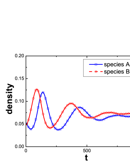
(a) Minority population densities.

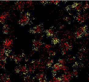
(b) Lattice snapshot at $t=1000$ mcs.

Figure 1: (Color online.) (a) Temporal evolution for the population densities of the minority species $A$ and $B$ for an asymmetric RPS system with rates $\lambda=0.8$ and $\sigma=\mu=0.07$ on a square lattice with $N=256\times 256$ sites, periodic boundary conditions, and initial densities $a(0)=b(0)=0.05$, $c(0)=0.9$; the data are averaged over 50 simulation runs. (b) Corresponding snapshot of the spatial particle distribution at $t=1000$ mcs (yellow/light gray: $A$, red/gray: $B$, black: $C$); note that there is no empty site in the lattice, since $\rho=a(0)+b(0)+c(0)=1$ is conserved under the temporal evolution.

In Fig. 1a, the population densities for the minority species $A$ and $B$ in an asymmetric “corner” RPS system model on a square lattice with rates $\lambda=0.8$ and $\sigma=\mu=0.07$ are plotted as functions of simulation time $t$ (in mcs). While the population densities for species $A$ and $B$ as obtained from the mean-field approximation for the RPS model would be identical, $\frac{\rho}{\lambda+\sigma+\mu}(\sigma,\ \mu)\approx(0.074,\ 0.074)$, the corresponding population densities in the associated LV model assume unequal values, $(a_{s},b_{s})=(0.065,0.075)$ in the (quasi-)steady state. The LV predictions are remarkably close to the measured values $(0.064\pm 0.003,0.074\pm 0.002)$ (averaged over 50 runs at $t=1000$ mcs, see Fig. 1a), clearly distinct for species $A$ and $B$. In particular, the persistent unequal population densities (starting from $t\approx 600$ mcs in Fig. 1a) support the population density inequality for minority species $A$ and $B$ in the (quasi-)steady state as statistically reliable. At the beginning of the simulations, we observe marked population oscillations, see Fig. 1a, reflecting the formation of complex spatio-temporal structures, i.e., expanding activity fronts as familiar in the stochastic spatial LV system, noticeable as minority species clusters in Fig. 1b. The emergence of such localized species clusters promotes species coexistence, reduces the oscillation amplitudes in the system, and eventually allows the system to evolve into the (quasi-)steady coexistence state. In light of these observations, we conclude that the temporal evolution of the two minority species $A$ and $B$ in the stochastic spatial corner RPS model with strongly asymmetric rates can indeed be faithfully approximated by the predator-prey behavior in the related two-species LV model. We shall further support this assertion through additional observations in the following subsection.

3.2 Fitness enhancement of the minority species due to spatial variability in the corner RPS model

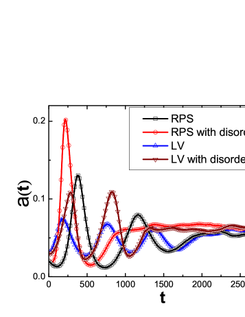
(a) Temporal evolution $a(t)$.

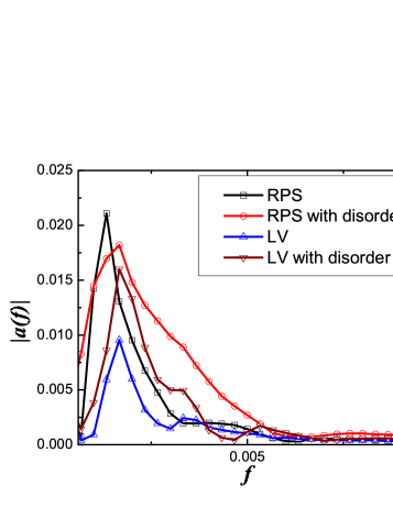
(b) Fourier transform $|a(f)|$.

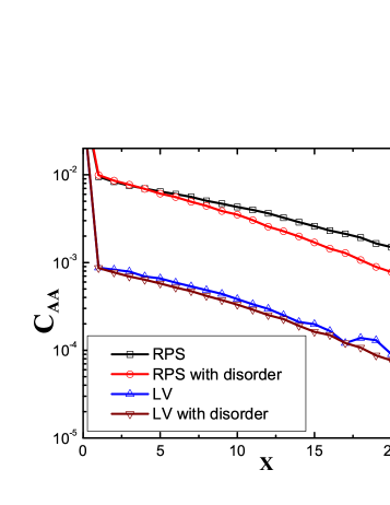
(c) Correlation function $C_{AA}(x)$.

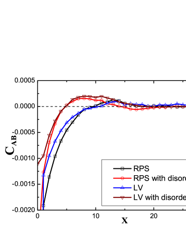
(d) Cross-correlation $C_{AB}(x)$.

Figure 2: (Color online.) Quantitative observables for a stochastic corner RPS model with rates $\lambda=0.5$, $\sigma=\mu=0.03$, and initial densities $a(0)=b(0)=0.02$, $c(0)=0.96$, and its corresponding LV system with $\lambda=0.5$, $\hat{\sigma}=\hat{\mu}=0.027$ and $a(0)=b(0)=0.03$ from simulation runs on a square lattice with $N=256\times 256$ sites (periodic boundary conditions). In the presence of spatial disorder, $\lambda\sim{\cal N}(0.5,0.4)$. All simulation results were averaged over 50 runs, and the correlation functions in (c) and (d) were measured at $t=3000$ mcs.

In order to further and quantitatively characterize the connection between the strongly asymmetric corner RPS system and its corresponding effective LV model, we next study the influence of quenched spatial disorder on the evolution of either system. Since spatial variability turns out to have very similar effects on species $A$ and $B$, we mainly show the results associated with species $A$; a complete listing of data for characteristic observables is provided in Table 1. We depict the temporal evolution of the population density $a(t)=\langle n_{A}(j,t)\rangle$, its Fourier transform $a(f)$, and the spatial auto- and cross-correlation functions $C_{AA}$ and $C_{AB}$, respectively, in the (quasi-)steady state (here, obtained at $t=3000$ mcs) in Fig. 2. The default rates are set to $\lambda=0.5$, $\sigma=\mu=0.03$ in the corner RPS model, and correspondingly $\lambda=0.5$, $\hat{\sigma}=\hat{\mu}=0.027$ in the associated LV model, and $\lambda\sim{\cal N}(0.5,\ 0.4)$ in both corner RPS and LV systems with quenched spatial disorder in the rate $\lambda$. Note that within the mean-field approximation, the population density for species $A$ in the (quasi-) steady state is $a_{s}\approx 0.048$, and the characteristic critical predation rate threshold is $\lambda_{c}=0.027<\lambda$, guaranteeing that the associated LV system is located in the active (quasi-)steady coexistence region of the phase diagram; it is also worth noticing that the minimum predation rate in the model variants with quenched spatial disorder is $0.1$, which is still well above the critical threshold, eliminating the possibility of any species extinction in our large lattices, even in the presence of spatial rate variability.

Figure 2a shows the simulated average population densities as function of time for the minority species $A$ in both corner RPS and associated LV systems, in the absence and presence of quenched spatial disorder. In the stationary state, the $A$ species concentrations (averaged over 50 runs at $t=3000$ mcs) become $0.057$ for the corner RPS model, $0.060$ for the associated LV model, $0.063$ for the RPS model with quenched spatial disorder, and $0.068$ for LV model with spatial disorder (see Table 1). Thus, within the error bars, the population density ($0.057$) for species $A$ in the “pure” corner RPS model coincides with the simulation result ($0.060$) for the associated stochastic spatial LV model. Moreover, we observe that spatial variability in the corner RPS model enhances the fitness of the minority species, as measured by the asymptotic stationary concentrations, by $\sim 11\%$. This fitness enhancement is in qualitative accord with earlier investigations on the effect of quenched randomness in the predation rate for the the two-species LV model without site restriction Ulrich , but turns out to be quantitatively less significant than the $\sim 25\%$ found there; it is also slightly smaller than the $\sim 13\%$ enhancement obtained directly in our simulations of the two-species LV model with restricted site occupation number, see Fig. 2a and Table 1.

We may attribute these differences to the fact that spatial disorder also affects the stationary population density $c^{*}$ of the majority species $C$ in the (quasi-)steady state of the corner RPS model, which in turn implies locally varying effective rates $\hat{\sigma}$ and $\hat{\mu}$ for the associated two-species LV model. This becomes apparent already on the mean-field description level, where $c^{*}=\frac{\lambda}{\lambda+\sigma+\mu}$ and $\hat{\sigma}=\sigma c^{*}$, $\hat{\mu}=\mu c^{*}$. Then for the minority species concentration deep in the coexistence state of the corner RPS model one obtains $a_{s}\approx\frac{\hat{\sigma}}{\lambda}=\frac{\sigma}{\lambda+\sigma+\mu}$. Similarly, for the two-species LV model with site restrictions, $a_{s}\approx\frac{\sigma}{\lambda+\sigma}$, whereas $a_{s}=\frac{\sigma}{\lambda}$ in the LV model with infinite local carrying capacity. In the latter case, a broad distribution of predation rates $\lambda$ strongly biases the system towards small values that considerably enhance the associated (quasi-)steady state density of $A$ species Ulrich . For the RPS system or the LV model subject to site occupation restrictions, the additional rates in the denominators reduce the significance of this low-$\lambda$ bias and ensuing concentration enhancement, and consequently the overall fitness enhancement is less pronounced.

As one would expect, the emergence of species clusters results in remarkable population oscillations at the beginning of the simulation runs, as seen in Fig. 2a. However, as shown in Fig. 2a, the transient period for the system evolving from the initial to the eventual active (quasi-)steady state is quite distinct for the different models. The corresponding Fourier-transformed density signal, which reflects both the characteristic oscillation frequency in the steady state and the associated characteristic relaxation time, is displayed in Fig. 2b. The Monte Carlo simulations exhibit the same peak frequency in the (quasi-) steady state for all four models, $f\approx 0.0014$; this characteristic peak frequency in the stochastic lattice systems is markedly reduced by $\sim 60\%$ as compared with the (linearized) mean-field prediction $f\approx\sqrt{\hat{\mu}\hat{\sigma}}/(2\pi)\approx 0.0043$. This remarkable decrease in the typical population oscillation frequency can be attributed to the renormalization by stochastic fluctuations in the spatial system Washenberger ; MauroGeorgiev2 ; Tauber . Moreover, the relaxation time $\tau=1/\Gamma$, where $\Gamma$ denotes the full width at half maximum of the oscillation peak in Fourier space, characterizes the typical time scale for the system to relax towards the (quasi-)steady state, and thus represents a measure of stability for these systems against external perturbations. Significantly, as demonstrated by the data in Fig. 2b and Table 1, the relaxation time in the RPS model with quenched spatial disorder is reduced by $\sim 50\%$ to $\sim 800$ mcs as compared with $\tau\sim 1800$ mcs in the corner RPS model without spatial rate variability.

	$a_{s}$	$b_{s}$	$\tau_{A/B}$	$l_{AA}$	$l_{BB}$	$l_{AB}$
RPS model	0.057 $\pm$ 0.003	0.060 $\pm$ 0.002	$\sim$ 1800 mcs	13.2 $\pm$ 0.6	16.0 $\pm$ 2.0	$\sim$ 13.0
RPS with disorder	0.063 $\pm$ 0.002	0.067 $\pm$ 0.003	$\sim$ 800 mcs	9.4 $\pm$ 0.2	13.0 $\pm$ 1.0	$\sim$ 8.0
LV model	0.060 $\pm$ 0.003	0.063 $\pm$ 0.003	$\sim$ 2000 mcs	12.8 $\pm$ 0.5	15.5 $\pm$ 0.5	$\sim$ 13.0
LV with disorder	0.068 $\pm$ 0.002	0.070 $\pm$ 0.003	$\sim$ 1300 mcs	10.3 $\pm$ 0.3	11.2 $\pm$ 0.2	$\sim$ 9.0

Table 1: Characteristic physical quantities measured by Monte Carlo simulations for the four stochastic spatial RPS and LV models whose features are displayed in Fig. 2. The population densities ($a_{s},b_{s}$) in the (quasi-)steady state are obtained as the averages over 50 simulation runs at $t=3000$ mcs (see Fig. 2a), the associated errors are measured as the standard deviations of the 50 data; and the relaxation time $\tau$ is found as the inverse of the full width at half maximum of the frequency peak in Fig. 2b. The correlation lengths $l_{AA}$ and $l_{BB}$ are extracted by fitting the simulation data for $C_{AA}$ and $C_{BB}$ to exponential functions (see Fig. 2c); and the separation length $l_{AB}$ is measured as the site location with the maximum value for $C_{AB}$ (see Fig. 2d).

The enhancement of both predator and prey fitness resulting from spatial variability in the stochastic lattice LV model is based on the emergence of more localized correlated spatio-temporal structures Ulrich . In all four model systems investigated here, such species clustering appears as well, see Fig. 1b. Compared to the RPS/LV model without spatial disorder, the corresponding RPS/LV system with spatial variability in the reaction rate $\lambda$ displays larger initial oscillation amplitudes (c.f. Fig. 2a), implying that spatial disorder in the predation rate tends to gather species closer, resulting in more localized and thus enhanced population growth spurts. To better understand the underlying spatial structures in our systems, we depict the static two-point auto-correlation functions in Fig. 2c and cross-correlation functions in the (quasi-) steady state in Fig. 2d. From these plots, we extract the typical correlation length $l_{AA}$, which measures the spatial extent of species $A$ clusters by fitting the simulation data $C_{AA}$ with an exponential function $\exp(-|x|/l_{AA})$, and obtain the predator-prey separation length $l_{AB}$, defined as the location where $C_{AB}$ assumes its maximum positive value. In the corner RPS model, the correlation and separation lengths turn out to be $l_{AA}=13.2$ (in units of lattice spacing) and $l_{AB}=13.0$, respectively, both of which coincide within the statistical error bars with the simulation results for the associated LV model, for which we find $l_{AA}=12.8$ and $l_{AB}=13.0$, as listed in Table 1. However, in the corresponding disordered RPS system, we measure markedly reduced values for the correlation and separation lengths, namely $9.4$ and $8.0$. This closer clustering near sites with locally favorable rates permits an overall larger number of population centers, and consequently enhances the net population densities for the minority species in the system with spatial variability in the rate $\lambda$.

In summary, as suggested on the basis of mean-field considerations, we find that the minority species $A$ and $B$ in our spatially extended stochastic RPS model with strongly asymmetric rates behave like the predator and prey in the coexistence phase of the two-species Lotka–Volterra model. Indeed, similar to our earlier findings for the lattice LV model Ulrich , we observe that quenched spatial disorder can markedly enhance the fitness of both minority species. This feature distinguishes the corner RPS model from the perhaps more common RPS system with comparable reaction rates, whose stationary state resides close to the center of configuration space; in that situation, quenched spatial reaction rate disorder hardly influences the dynamical evolution of either species Qian ; QianEPJB .

4 Hierarchical three-species “food chain” model

In Section 3, we have demonstrated how the properties of the coexistence state in the two-species Lotka–Volterra model emerge as the rock–paper–scissors system is moved towards one of the corners of configuration space by choosing strongly asymmetric rates. Another natural idea to generate the LV model is to consider a hierarchical three-species “food chain” system, where an intermediate species $C$ is inserted between the predators $A$ and prey $B$. The question then becomes: will a stochastic hierarchical three-species food chain model on a lattice in a certain limit again recover the properties of the spatial two-species LV system? To this end, we investigate the following coupled stochastic reactions that define our three-species food chain:

$$A\to \emptyset\qquad \quad{\rm with\ rate}\ \mu\ ;$$

$$A+C\to A+A \quad{\rm with\ rate}\ \lambda\ ;$$

$$C+B\to C+C \quad{\rm with\ rate}\ \lambda\ ;$$ (11)

$$B\to B+B \quad{\rm with\ rate}\ \sigma\ .$$

Species $A$ and $B$ in this model behave as predators and prey, respectively, while the intermediate population $C$ preys on species $B$ and is preyed upon by species $A$. In order to perhaps closely approach the two-species LV system and mainly study the dynamic behavior of species $A$ and $B$, we here use identical reaction rates $\lambda$ for the $A$-$C$ and $B$-$C$ predation processes. We remark that upon identifying the empty state with a fourth species, this system can be mapped onto a cyclic four-species predator-prey model, see, e.g., Refs. Durney ; Dobrinevski , with a peculiar choice of rates. In our Monte Carlo simulations for a spatially extended system on a square lattice with periodic boundary conditions, we allow at most one particle per site. The resulting mean-field rate equations now read:

$$\partial_{t}\,a(t) = a(t)\left[\lambda\,c(t)-\mu\right]\ ,$$

$$\partial_{t}\,c(t) = \lambda\,c(t)\left[b(t)-a(t)\right]\ ,$$ (12)

$$\partial_{t}\,b(t) = \sigma\,b(t)\left[1-a(t)-b(t)-c(t)\right]-\lambda\,b(t)c(t)\ ,$$

since only the reproduction process for the species $B$ requires the presence of an empty site in its immediate neighborhood, whereas newly generated $A$ and $C$ particles just replace their respective prey. As stationary solutions of the coupled rate equations (12), one finds one linearly unstable absorbing point $(a,c,b)=(0,0,1)$, an entire absorbing line $(0,c,0)$, where $c\in[0,1]$, and one active coexistence fixed point:

$$(a_{s},c_{s},b_{s})=\left(\frac{\lambda\sigma-\mu(\lambda+\sigma)}{2\lambda\sigma}\ ,\frac{\mu}{\lambda}\ ,\frac{\lambda\sigma-\mu(\lambda+\sigma)}{2\lambda\sigma}\right).\quad$$ (13)

As in the two-species LV model with site occupation restrictions, there exists a critical threshold for the predation rate $\lambda_{c}=\frac{\mu\sigma}{\sigma-\mu}$ in this hierarchical food chain model, where in the thermodynamic limit a phase transition occurs from the inactive absorbing states to the active coexistence state: When the predation rate is below the threshold ($\lambda<\lambda_{c}$), the system evolves towards extinction for the $A$ and $B$ population $(0,c,0)$; otherwise, the system eventually reaches the three-species coexistence state $(a_{s},c_{s},b_{s})$. However, in stark contrast with the mean-field analysis for the two-species LV model with site restrictions, the population densities for the predators $A$ and the prey $B$ in this food chain system are always the same in the stationary coexistence state, in order for the intermediate species $C$ to possess a nonzero stationary population density. Other important distinct spatio-temporal properties for the spatially extended hierarchical food chain model will be discussed in the following two subsections.

4.1 Monte Carlo simulations: mean-field like behavior

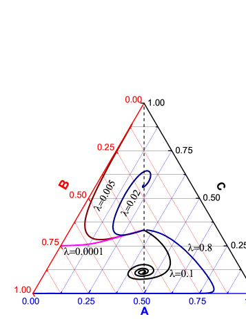
(a) Normalized evolution trajectories

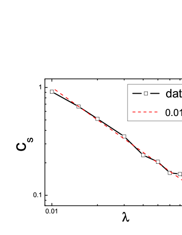
(b) $c_{s}\sim 1/\lambda$ in the (quasi-)steady state

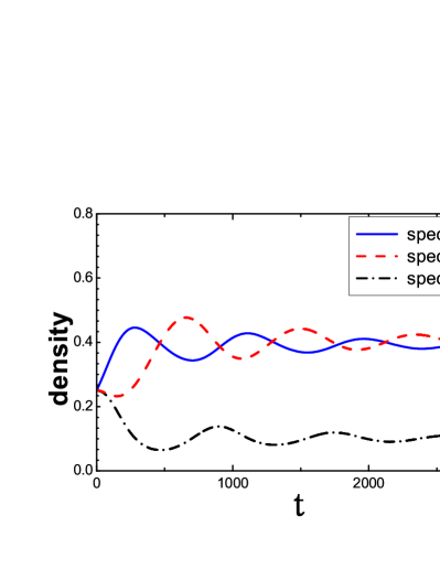
(c) Population densities for $\lambda=0.1$

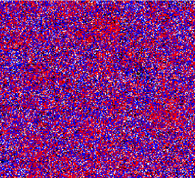
(d) Snapshot at $t=3000\ mcs$ for $\lambda=0.1$

Figure 3: (Color online.) Observables for a stochastic three-species hierarchical food chain system in two dimensions with $N=256\times 256$ sites, reaction rates $\mu=0.01,\sigma=0.1$, and $\lambda$ as indicated; the simulations started with equal initial densities $a(0)=b(0)=c(0)=1/3$ in (a) and (b), and $a(0)=b(0)=c(0)=0.25$ in (c) and (d); the data were averaged over 50 simulation runs; color coding in (d): blue/dark gray: $A$, red/gray: $B$, black: $C$, white: empty.

In the Monte Carlo simulation runs, we first permit both nearest-neighbor particle exchange and hopping processes to generate population spreading. In Fig. 3a, we depict the typical normalized trajectories for the population densities in systems with varying predation rates $\lambda$. The other rates $\mu=0.01$, $\sigma=0.1$ are unchanged, whence the critical predation rate threshold value remains fixed at $\lambda_{c}=\frac{\mu\sigma}{\sigma-\mu}\approx 0.011$. When the predation rate is below this threshold, the trajectories ($\lambda=0.0001,0.005$ in Fig. 3a) reach the boundaries in the phase space spanned by the the population densities, which constitute inactive absorbing states. Upon increasing the predation rate ($\lambda=0.02,0.1$ in Fig. 3a), we observe that the system evolves to the active coexistence state. While for small predation rates just above the threshold ($\lambda=0.02$ in Fig. 3a) the fixed point is a node, it changes character and becomes a spiral focus for larger values, as evidenced by the spiral trajectory in the phase graph ($\lambda=0.1$ in Fig. 3a). This fixed point evolution as function of the predation rate is remarkably similar to the situation in two-species LV model with site restriction MauroGeorgiev2 . As discussed earlier, in the active coexistence state the predator $A$ and prey $B$ species should possess the same population densities in order to let the intermediate species $C$ also have nonzero stationary population density (see the dashed line in Fig. 3a). However, when $\lambda$ becomes large relative to the rate $\mu$ ($\lambda=0.8$ in Fig. 3a), the population density of the intermediate species $C$ in the (quasi-)steady state is reduced so much ($c_{s}=\frac{\mu}{\lambda}\approx 0.01$ in the figure) that the strong stochastic population oscillations cause the evolution trajectories to touch the absorbing phase boundary; thus, the simulation eventually terminates at one of the absorbing states on the lines $(a,0,b)$ which are not apparent in the mean-field analysis.

Furthermore, as shown in Fig. 3b, the quantitive relationship between the population density $c_{s}$ for the intermediate species $C$ in the active coexistence state and the predation rate $\lambda$ numerically agrees remarkably well with the mean-field prediction $c_{s}=\mu/\lambda$. In Fig. 3c, we plot the temporal evolution of the three species’ population densities for runs with predation rate $\lambda=0.1$; the population densities in the (quasi-)steady state (averaged over 50 runs at $t=3000$ mcs) are found to be $(0.4\pm 0.01,0.1\pm 0.003,0.4\pm 0.01)$, again fully consistent with the predictions of the mean-field approximation. We also numerically investigated the influence of quenched spatial disorder on the dynamical evolution of the system. However, in stark contrast with the robust fitness enhancement in the two-species LV model, in the hierarchical three-species model spatial variability in the predation rate $\lambda$ does not generate any noticeable effect on the dynamical evolution of the system. These observations are further elucidated by the spatial distribution snapshot on a two-dimensional lattice depicted in Fig. 3d: All particles appear randomly scattered on the lattice in the (quasi-)steady state, and no correlated spatio-temporal structures such as either clusters or spirals become manifest. Consequently quenched spatial disorder cannot beneficially affect any correlations as in the LV model.

Our Monte Carlo simulations demonstrate that the spatial three-species hierarchical food chain system, with both nearest-neighbor particle pair exchange and hopping processes present, is quantitatively well-described by the mean-field approximation. In the following subsection, we thus explore the respective role of particle pair exchange vs. hopping processes.

4.2 Particle pair exchange processes and pure hopping processes

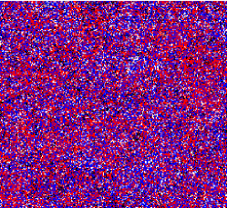
(a) Particle pair exchange processes

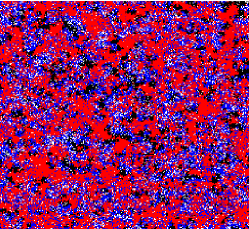
(b) Nearest-neighbor hopping

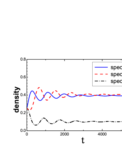
(c) Temporal evolution for (a)

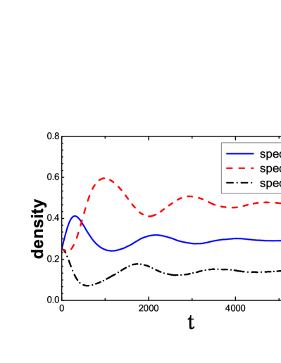
(d) Temporal evolution for (b)

Figure 4: (Color online.) (a) and (b): Snapshots of the spatial particle distribution at $t=6000$ mcs for a stochastic three-species hierarchical food chain system with $N=256\times 256$ sites, reaction rates $\lambda=0.1$, $\mu=0.01$, and $\sigma=0.1$, starting with equal initial densities $a(0)=b(0)=c(0)=0.25$. Blue/dark gray: $A$, red/gray: $B$, black: $C$, white: empty. (c) and (d): Temporal evolution of population densities for simulation runs with (a) only nearest-neighbor particle exchange, and (b) only nearest-neighbor hopping, with $N=100\times 100$ sites, averaged over 50 simulation runs.

In the above subsection, we have demonstrated that population spreading through both nearest-neighbor particle pair exchange and hopping processes can well mix the two-dimensional spatially extended three-species hierarchical food chain system. In order to further explore the origin for the appearance of mean-field behavior, we ran simulations wherein either the particle hopping or pair exchange processes were removed; Figs. 4a and 4b show snapshots of the resulting (quasi-)stationary particle distributions. In Fig. 4a where only nearest-neighbor particle pair exchange was allowed, it is seen that the individuals for each species are uniformly distributed on the lattice, and no particular spatial patterns emerge in the system. We depict the associated temporal evolution (up to $6000$ mcs) of the three population densities for a smaller system ($N=100\times 100$) in Fig. 4c. The population densities $(0.39\pm 0.01,0.10\pm 0.01,0.40\pm 0.02)$ in the (quasi-) steady state (averaged over 50 runs at $t=6000$ mcs) are again quantitatively consistent with the mean-field predictions. Also, as one would expect, we have not observed any remarkable influence of quenched spatial disorder on the evolutionary dynamics in these systems.

Next, we investigate systems wherein particle spreading occurs solely through nearest-neighbor hopping, see Figs. 4b and 4d. In Fig. 4b, one notices distinct species clusters, as also observed in two-species LV systems; however, it is worthwhile noting that interactions between predators $A$ and prey $B$ do not directly take place at their respective cluster boundaries, but can only be indirectly realized via interspersed clusters of the intermediate species $C$ (visible as black patches in Fig. 4b). The required presence of the intermediate species clusters significantly coarse-grains the indirect reactions between predators $A$ and prey $B$, and effectively averages over spatially correlated structures. Again, we find that quenched spatial disorder does not noticeably affect the evolutionary dynamics of the system. However, as shown in Fig. 4d, the population densities $(0.29\pm 0.01,0.14\pm 0.01,0.47\pm 0.02)$ in the (quasi-) steady state (averaged over 50 runs at $t=6000$ mcs) do not coincide with the predictions from the mean-field rate equations, i.e., nearest-neighbor hopping processes alone are not strong enough to effectively mix the two-dimensional three-species hierarchical food chain system. We have furthermore checked that these numerical observations, here obtained for $\lambda=0.1$, about the effect of either particle pair exchange processes or pure hopping processes also apply to systems with much smaller predation rate $\lambda=0.02$.

In summary, we have demonstrated that the hierarchical three-species food chain model with site restrictions and with particle spreading through pair exchange processes effectively washes out the formation of any spatial structures, hence becomes well mixed, and behaves as in the mean-field predictions. As is also observed in the two-species LV system with site restrictions, the hierarchical food chain model also possesses a critical threshold for the predation rate, where a phase transition from an inactive absorbing state to an active coexistence state occurs. However, if particle spreading happens solely through nearest-neighbor hopping, distinct species clusters emerge. Yet since intermediate species $C$ clusters are necessary to indirectly promote predation interactions between the $A$ and $B$ species, the effective reaction boundaries between the predators and prey become blurred, such that any spatial variability still cannot remarkably influence the dynamical evolution of these food chain systems. Consequently, at least for the parameter values and system sizes studied here, the ensuing hierarchical three-species food chain model does not closely resemble the features of the corresponding two-species spatial stochastic LV system that is governed by strong fluctuations and marked correlations in the active coexistence state.

5 Conclusion

In this paper, we studied the connection between two three-species predator-prey systems and the well-understood two-species Lotka–Volterra model. First, we explored the evolutionary behavior of the two minority species in the “corner” three-species cyclic rock–paper–scissors (RPS) model with strongly asymmetric rates. We analytically demonstrate that in the mean-field limit the evolutionary dynamics of both minority species in the “corner” RPS model can be well approximated by the two-species LV model. Employing Monte Carlo simulation for a two-dimensional spatially extended “corner” RPS model, we found the population densities for those two minority species in the (quasi-)steady state to coincide with both the analytic predictions from mean-field approximation in the resulting two-species LV model and its associated numerical simulation results. Furthermore, introducing quenched spatial disorder into the predation rate $\lambda$ in the “corner” RPS model, we observe that the influence of quenched spatial disorder on the evolution of system cannot be ignored, in contrast to RPS systems far away from the “corner” of configuration space, wherein quenched spatial disorder has only minor effects on the evolution of the system Qian : The minority species’ fitness in the “corner” RPS system is markedly enhanced due to the spatial variability in the predation rates, as is indicated by larger population densities for both minority species in the (quasi-)steady state, and accompanied by shorter relaxation times and stronger localization of the clusters for those two minority species. That is, the two minority species in the “corner” RPS model behave just like the predator and prey in the spatially extended two-species LV system.

We also investigated hierarchical three-species “food chain” systems, in which an additional intermediate species is inserted between the predators and prey in the classic two-species LV model. As observed in the spatial version of the two-species LV model with site occupancy restrictions, in the similarly restricted three-species “food chain” model with finite total carrying capacity, there exists a critical predation rate threshold, which in the thermodynamic limit represents a non-equilibrium phase transition from an inactive absorbing to an active coexistence state. Our simulation results show that nearest-neighbor particle pair exchange processes are sufficient to wash out the formation of species clusters and consequently generate a well-mixed spatial system, whose features can be quantitatively well approximated by the mean-field rate equations, and wherein the influence of quenched spatial disorder may safely be ignored. Moreover, if we allow only nearest-neighbor hopping processes, and eliminate any pair exchanges, distinct species clusters appear in the coexistence state. However, due to the interruption by intermediate species clusters, the predation processes between predator and prey are effectively coarse-grained, and fluctuation and correlation effects on the resulting two-species dynamics suppressed. Consequently, quenched spatial disorder still cannot enhance the fitness of either species. That is, as opposed to the “corner” rock-paper-scissors model with strongly asymmetric rates, the spatially extended hierarchical three-species “food chain” system actually does not behave like the two-species LV model.

This work is in part supported by Virginia Tech’s Institute for Critical Technology and Applied Science (ICTAS) through a Doctoral Scholarship, and the US National Science Foundation through grant No. DMR-1005417. We gratefully acknowledge inspiring discussions with Uli Dobramysl and Michel Pleimling.

References

- (1) J. Maynard Smith, Evolution and the Theory of Games (Cambridge University Press, Cambridge, U.K., 1982)
- (2) J. Hofbauer and K. Sigmund, Evolutionary Games and Population Dynamics (Cambridge University Press, Cambridge, U.K., 1998)
- (3) M. A. Nowak, Evolutionary Dynamics (Belknap Press, Cambridge, USA, 2006)
- (4) R. M. May and W. J. Leonard, SIAM J. Appl. Math. 29, 243-253 (1975)
- (5) R. M. May, Stability and Complexity in Model Ecosystems (Cambridge University Press, Cambridge, U.K., 1974)
- (6) J. Maynard Smith, Models in Ecology (Cambridge University Press, Cambridge, U.K., 1974)
- (7) R. E. Michod, Darwinian Dynamics (Princeton University Press, Princeton, USA, 2000)
- (8) R. V. Sole and J. Basecompte, Self-Organization in Complex Ecosystems (Princeton University Press, Princeton, USA, 2006)
- (9) D. Neal, Introduction to Population Biology (Cambridge University Press, Cambridge, U.K., 2004)
- (10) A. J. Lotka, Proc. Natl. Acad. Sci. U.S.A 6 410 (1920); J.Amer. Chem.Soc.42 1595 (1920)
- (11) V. Volterra, Mem. Accad. Lincei 2 31 (1926); Lecons sur la théorie mathématique de la lutte pour la vie (Paris: Gauthiers-Villars, 1931)
- (12) R. Monetti, A. F. Rozenfeld and E. V. Albano, Physica A 283, 52 (2000)
- (13) E. Bettelheim, O. A. Nadav and N. M. Shnerb, Physica E 9, 600 (2001)
- (14) M. Droz and A. Pekalski, Phys. Rev. E 63, 051909 (2001)
- (15) T. Antal and M. Droz, Phys. Rev. E 63, 056119 (2001)
- (16) M. Kowalik, A. Lipowski and A. L. Ferreira, Phys. Rev. E 66, 066107 (2002)
- (17) A. J. McKane and T. J. Newman, Phys. Rev. Lett. 94, 218102 (2005)
- (18) M. J. Washenberger, M. Mobilia and U. C. Täuber, J. Phys.: Condens. Matter 19, 065139 (2007)
- (19) M. Mobilia, I. T. Georgiev and U. C. Täuber, J. Stat. Phys. 128, 447 (2007)
- (20) G. Szabó and G. Fáth, Phys. Rep. 446, 97 (2007)
- (21) S. Venkat and M. Pleimling, Phys. Rev. E 81, 021917 (2010)
- (22) L. Frachebourg, P. L. Krapivsky and E. Ben-Naim, Phys. Rev. E 54, 6186 (1996)
- (23) B. Sinervo and C. M. Lively, Nature (London) 380, 240 (1996)
- (24) K. R. Zamudio and B. Sinervo, Proc. Natl. Acad. Sci. (USA) 97, 14427 (2000)
- (25) B. Kerr, M. A. Riley, M. W. Feldman and B. J. M. Bohannan, Nature (London) 418, 171 (2002)
- (26) T. Reichenbach, M. Mobilia and E. Frey, Nature (London) 448, 1046 (2007)
- (27) T. Reichenbach, M. Mobilia and E. Frey, Phys. Rev. Lett. 99, 238105 (2007)
- (28) T. Reichenbach, M. Mobilia and E. Frey, J. Theor. Biol. 254, 368 (2008)
- (29) J. D. Murray, Mathematical Biology Vols. I, II (Springer, New York, USA, 2002)
- (30) U. Dobramysl and U. C. Täuber, Phys. Rev. Lett. 101, 258102 (2008)
- (31) A. Lipowski and D. Lipowska, Physica A 276, 456 (2000)
- (32) A. F. Rozenfeld and E. V. Albano, Physica (Amsterdam) 266A, 322 (1999)
- (33) J. E. Satulovsky and T. Tom, Phys. Rev. E 49, 5073 (1994)
- (34) N. Boccara, O. Roblin and M. Roger, Phys. Rev. E 50, 4531 (1994)
- (35) A. Lipowski, Phys. Rev. E 60, 5179 (1999)
- (36) D. Panja, Phys. Rep. 393, 87 (2004)
- (37) L. O’Malley, B. Kozma, G. Korniss, Z. Rcz and T. Caraco, Phys. Rev. E 74, 041116 (2006)
- (38) S. R. Dunbar, J. Math. Biol. 17, 11 (1983)
- (39) J. Sherratt, B. T. Eagen and M. A. Lewis, Phil. Trans. R. Soc. Lond. B 352, 21 (1997)
- (40) M. A. M. de Aguiar, E. M. Rauch and Y. Bar-Yam, J. Stat. Phys. 114, 1417 (2004)
- (41) A. Provata, G. Nicolis and F. Baras, J. Chem. Phys. 110, 8361 (1999)
- (42) M. Mobilia, I. T. Georgiev and U. C. Täuber, Phys. Rev. E 73, 040903(R) (2006)
- (43) T. Reichenbach, M. Mobilia and E. Frey, Banach Center Publications Vol. 80, 259 (2008)
- (44) T. Reichenbach, M. Mobilia and E. Frey, Phys. Rev. E 74, 051907 (2006)
- (45) M. Berr, T. Reichenbach, M. Schottenloer and E. Frey, Phys. Rev. Lett. 102, 048102 (2009)
- (46) K. I. Tainaka, Phys. Rev. E 50, 3401 (1994)
- (47) G. Szabó and A. Szolnoki, Phys. Rev. E 65, 036115 (2002)
- (48) M. Perc, A. Szolnoki and G. Szabó, Phys. Rev. E 75, 052102 (2007)
- (49) G. A. Tsekouras and A. Provata, Phys. Rev. E 65, 016204 (2001)
- (50) Q. He, M. Mobilia and U. C. Täuber, Eur. Phys. J. B 82, 97 (2011)
- (51) M. Frean and E. R. Abraham, Proc. R. Soc. London, Ser. B 268, 1323 (2001)
- (52) Q. He, M. Mobilia and U. C. Täuber, Phys. Rev. E 82, 051909 (2010)
- (53) M. Peltomäki and M. Alava, Phys. Rev. E 78, 031906 (2008)
- (54) R. K. P. Zia, e-print arXiv: 1101.0018 (2011)
- (55) U. C. Täuber, J. Phys.: Conf. Ser. 319, 012019 (2011)
- (56) C. H. Durney, S. O. Case, M. Pleimling and R. K. P. Zia, Phys. Rev. E 83, 051108 (2011)
- (57) A. Dobrinevski and E. Frey, e-print arXiv: 1001.5235 (2010)