Modeling Amphiphilic Solutes in a Jagla Solvent

Abstract

Methanol is an amphiphilic solute whose aqueous solutions exhibit distinctive physical properties. The volume change upon mixing, for example, is negative across the entire composition range, indicating strong association. We explore the corresponding behavior of a Jagla solvent, which has been previously shown to exhibit many of the anomalous properties of water. We consider two models of an amphiphilic solute: (i) a “dimer” model, which consists of one hydrophobic hard sphere linked to a Jagla particle with a permanent bond, and (ii) a “monomer” model, which is a limiting case of the dimer, formed by concentrically overlapping a hard sphere and a Jagla particle. Using discrete molecular dynamics, we calculate the thermodynamic properties of the resulting solutions. We systematically vary the set of parameters of the dimer and monomer models and find that one can readily reproduce the experimental behavior of the excess volume of the methanol-water system as a function of methanol volume fraction. We compare the pressure and temperature dependence of the excess volume and the excess enthalpy of both models with experimental data on methanol-water solutions and find qualitative agreement in most cases. We also investigate the solute effect on the temperature of maximum density and find that the effect of concentration is orders of magnitude stronger than measured experimentally.

I INTRODUCTION

Aqueous solutions of alcohols have attracted both experimental and theoretical attention on account of their ubiquity and importance in the medical, personal care, transportation (e.g., antifreeze, fuels), and food industries, among others AkerlofJAC1932 ; GibsonJAC1935 ; FrankJCP1945 ; LamaJCED1965 ; BensonJSC1980 ; KubotaIJT1987 ; TomaszkiewiczTA1986II ; TomaszkiewiczTA1986III ; XiaoJCT1997 ; Mcglashan1976 ; SatoJCP2000 . Methanol is a simple example of an amphiphilic organic solute, and its aqueous solutions exhibit many interesting nonidealities. Attaining a good understanding of this simple case is therefore a natural starting point for studies of more complex solutes in water, such as higher alcohols or proteins.

Because of the increasing availability of expanded computing power, simulations have become an important research tool in studying aqueous methanol solutions MauroJCP1990 ; HidekiJCP1992 ; EickJCP2003 ; Diego2006 ; Imre2008 ; YangJCC2007 . The optimized potential for liquid simulation (OPLS) JorgensenJPC1986 is frequently used to model alcohol molecules. To represent water as a solvent, the SPC/E BerendsenJPC1987 , TIP3P JorgensenJCP1983 , TIP4P JorgensenMP1985 , and TIP5P MahoneyJCP2000 models are frequently used. On the other hand, many thermodynamic properties of water can be reproduced using soft-core spherically symmetric potentials, one of the most important of which is the Jagla model JaglaPRE2001 . The Jagla potential has a hard core and a linear repulsive ramp, and contains two characteristic length scales: a hard core $a$ and a soft core $b$. For a range of parameters, the Jagla model exhibits a water-like ErringtonNature2001 cascade of structural, transport, and thermodynamic anomalies JaglaPRE2001 ; YanPRL2005 ; LimeiPNAS2005 ; LimeiPRE2006 . Buldyrev et al. in 2007 SergeyPNAS2007 found that the Jagla solvent exhibits key water-like characteristics with respect to hydrophobic hydration, suggesting that the water-like characteristics of the Jagla solvent extend beyond the pure fluid. Here, we explore this analogy further, considering the properties of solutions of amphipathic solutes.

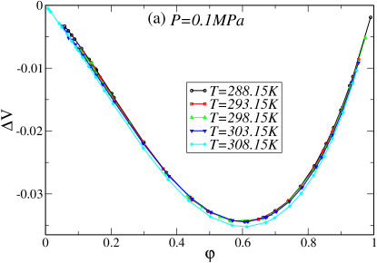
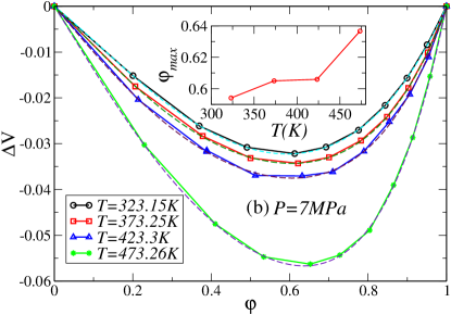
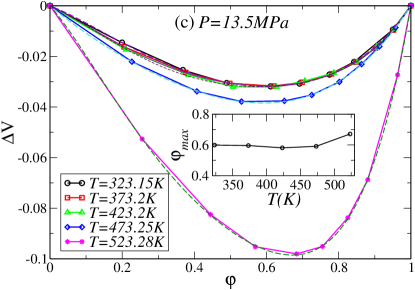
Figure 1: (color online) Experimental data BensonJSC1980 ; XiaoJCT1997 on the temperature dependence of the excess volume, as a function of the volume fraction of methanol, $\varphi$, at different pressures (Dotted lines are polynomial fits of experimental data): (a) $P=0.1$MPa, (b) $P=7$MPa, and (c) $13.5$MPa. Note that in (a) temperature interval between two measurements is 5K, while the temperature difference in (b) and (c) is 50K. The excess volume is the relative difference between the volume occupied by the mixture and the sum of the volumes of the pure components before mixing, at fixed temperature and pressure

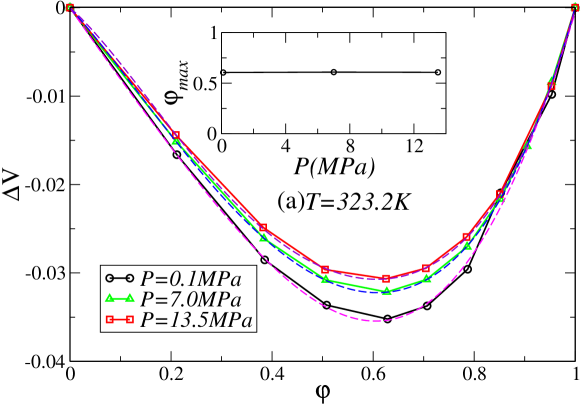
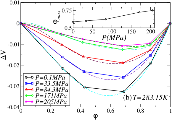
Figure 2: (color online) Experimental data XiaoJCT1997 ; KubotaIJT1987 on the pressure dependence of the excess volume as a function of the volume fraction of methanol, $\varphi$, at two different temperatures (dotted lines are polynomial fits of experimental data): (a)$T=323.2$K and (b) $T=285.15$K. Note that the range of the pressure shown in (a) is smaller than that in (b). The excess volume is defined in the caption of Fig. 1

We focus on the properties of the excess volume and the excess enthalpy, and on how amphiphilic solutes affect the temperature of maximum density ($T_{\rm MD}$) of a solution. At $T=298$K and $P=0.1$MPa the excess volume and the excess enthalpy are negative across the entire range of methanol concentrations (both quantities will be defined rigorously below). The strongest effect occurs at a methanol volume fraction of $\varphi_{\rm max}=59.7$%, at which the negative excess volume deviates from additivity by $-3.57$% Mcglashan1976 . As $T$ increases and $P$ decreases, the excess volume becomes more negative and the extremal point shifts (see Fig. 1 and Fig. 2). Most solutes tend to suppress water’s non-idealities, and hence they lower the $T_{\rm MD}$. Some amphiphilic solutes behave differently: ethanol and t-butanol have a marked non-monotonic effect (whereby the $T_{\rm MD}$ of the solution first increases with respect to that of water upon solute addition, but decreases for more concentrated solutions), and methanol has a very mild non-monotonic effect WadaBCSJ1962 .

As a first step , in this paper, our goal is to model a simple amphiphilic solution that mimics the properties of the methanol-water system. We use a hard sphere with parameterized diameter $a_{\rm M}$ to model the hydrophobic methyl group, and a Jagla particle to model the hydrophilic hydroxyl group. We link the hard sphere and the Jagla particle using a bond of adjustable length to model the amphiphilic solutes.

In Section II of this paper we describe in detail our models and simulation methods. In Section III we list and analyze the simulation results, and in its four subsections we discuss the different parameter effects, the temperature and pressure dependence of the excess volume, the behavior of the excess enthalpy, and how the solute concentration affects the temperature of maximum density. In Section IV we list our main conclusions.

II MODEL and METHODS

II.1 Dimer model for amphiphilic solutes

To model the simple amphiphilic solute methanol, we separate CH₃OH into the methyl (CH₃) and the hydroxyl (OH) groups. We model CH₃ as a hard sphere and OH as a Jagla particle. There is one bond between the hard sphere and the Jagla particle. We call this model the dimer model. To model the solvent, H₂O, we use the Jagla particle. The following interactions are included: there is a Jagla potential between Jagla solvent particles, a Jagla potential between the Jagla solvent and a dimer’s Jagla particle, and a Jagla potential between two dimer’s Jagla particles, all of which are denoted by $U_{\rm JJ}(r)$ [Fig. 3(a)]. The interaction between the hard spheres is modeled by a hard-core potential $U_{\rm HH}(r)$, and the interaction between the hard spheres and the Jagla particles is modeled by a hard core potential $U_{\rm JH}(r)$. We model the covalent bond with a narrow square well potential bounded by two hard walls $U_{\rm bond}(r)$. The interaction potentials are

$$U_{\rm JJ}(r)=\left\{\begin{array}[]{ll}\infty&r<a\\ -U_{o}+\frac{(U_{o}+U_{R})(b-r)}{b-a}&a<r<b\\ -U_{o}\frac{c-r}{c-b}&b<r<c\\ 0&r>c\end{array}\right.,$$ (1)

where $a$ is the hard core diameter, $b=1.72a$ is the soft core diameter, $c=3a$ is the range of attractive potential, $U_{o}$ is the maximum attractive energy and $U_{R}=3.56U_{o}$ is the maximum repulsive energy, and

$$U_{HH}(r)=\left\{\begin{array}[]{ll}\infty&r<a_{\rm M}\\ 0&r>a_{\rm M}\end{array}\right.,$$ (2)

where $a_{\rm M}$ is the diameter of the hard sphere, and

$$U_{JH}(r)=\left\{\begin{array}[]{ll}\infty&r<a_{\rm JM}\\ 0&r>a_{\rm JM}\end{array}\right.$$ (3)

where $a_{\rm JM}=\frac{a_{\rm M}+a}{2}$ and

$$U_{\rm bond}(r)=\left\{\begin{array}[]{ll}\infty&r<\zeta-\frac{\delta}{2}\\ 0&\zeta-\frac{\delta}{2}<r<\zeta+\frac{\delta}{2}\\ \infty&r>\zeta+\frac{\delta}{2}\end{array}\right.,$$ (4)

The hard core diameter $a_{\rm M}$ and the average length of the covalent bond $\zeta$ are used as adjustable parameters in order to achieve agreement between the excess volume of the model solution and the experimental results of methanol-water solutions at ambient conditions. In all our simulations, we use the same set of Jagla potential parameters, $b=1.72a$, $c=3a$, and $U_{R}=3.56U_{o}$ LimeiPRE2006 . We use reduced units in terms of length $a$, energy $U_{o}$, and particle mass $m$. For temperature we use units of $U_{o}/k_{B}$; for pressure we use units of $U_{o}/a^{3}$; and for volume we use units of $a^{3}$.

II.2 Monomer model for amphiphilic solutes

The best agreement between the dimer model and the experimental data occurs when bonds are short (for a more detailed discussion, see Sec. II), i.e., the hard sphere that models the methyl group and the Jagla particle that models the hydroxyl group almost overlap. For this reason we also consider a methanol model in which the overlap is complete, and the bond length vanishes. This leads to a spherically symmetric potential that superimposes the Jagla particle and the hard sphere. In this “monomer” model we introduce the interaction potentials between “methyl” monomers, $U_{\rm MM}(r)$ [Fig. 3(b)], between monomer and Jagla particle, $U_{\rm JM}(r)$ [Fig. 3(c)], and between Jagla particles $U_{\rm JJ}(r)$ [Fig. 3(a)]. In this case the interaction formulae are

$$U_{\rm MM}(r)=\left\{\begin{array}[]{ll}\infty&r<a_{\rm M}\\ U_{\rm JJ}(r)&r>a_{\rm M}\end{array}\right.,$$ (5)

and

$$U_{\rm JM}(r)=\left\{\begin{array}[]{ll}\infty&r<a_{\rm JM}\\ U_{\rm JJ}(r)&r>a_{\rm JM}\end{array}\right.,$$ (6)

where $U_{\rm JJ}(r)$ is defined by Eq. (1).

II.3 Simulation details and analysis methods

For our simulations we use the discrete molecular dynamics (DMD) algorithm. With DMD we approximate a continuous potential by a discrete potential made up of a series of steps. We use the same scheme as in Ref. LimeiPRE2006 . Our simulation consists of a fixed number $N=2000$ particles in a cubic box with periodic boundaries. We denote the solute mole fraction by $x$. Since the dimer contains two particles and the monomer one, the number of solute molecules $N_{s}(x)$ is

$$N_{s}(x)=\frac{Nx}{x+1}$$ (7)

in the dimer system, and

$$N_{s}(x)=Nx$$ (8)

in the monomer system. The number of the solvent particles $N_{J}(x)$ is

$$N_{J}(x)=\frac{N(1-x)}{x+1}$$ (9)

in the dimer system, and

$$N_{J}(x)=N(1-x)$$ (10)

in the monomer system. The total number of molecules in the system $N_{T}(x)$ is

$$N_{T}(x)=\frac{N}{x+1}$$ (11)

in the dimer model, and

$$N_{T}(x)=N$$ (12)

in the monomer model. The volume occupied by $N_{J}(x)$ pure Jagla solvent particles before mixing, $V_{J}(x)$, and the volume occupied by $N_{s}(x)$ pure solute molecules before mixing, $V_{s}(x)$, at the given temperature and pressure, are given by

$$V_{J}(x)=\frac{N_{J}(x)}{N_{J}(0)}V_{\rm mix}(0)$$ (13)

and

$$V_{s}(x)=\frac{N_{s}(x)}{N_{s}(1)}V_{\rm mix}(1),$$ (14)

where $V_{\rm mix}(x)$ is the volume of the mixture with mole fraction $x$.

We define the excess volume of the solution with respect to the ideal mixture as

$$\bigtriangleup V=\frac{V_{\rm mix}(x)}{V_{J}(x)+V_{s}(x)}-1$$ (15)

If the excess volume $\bigtriangleup V$ is negative, the volume of the solution is less than the volume of the ideal mixture. If it is positive, the system expands after mixing at fixed temperature and pressure. In most contexts, we use the volume fraction

$$\varphi=\frac{V_{s}(x)}{V_{J}(x)+V_{s}(x)}$$ (16)

rather than the mole fraction $x$ to express different solute concentrations of solutions.

We compare our simulation results with the data from experiments LamaJCED1965 ; Mcglashan1976 , where the excess volume is expressed in terms of $\bigtriangleup Y=\frac{V_{mix}-(n_{w}v_{w}+n_{m}v_{m})}{n_{w}+n_{m}}$, where $n_{m}$ is the number of the moles of methanol, $n_{w}$ is the number of moles of water, the mole fraction is $x=\frac{n_{m}}{n_{w}+n_{m}}$, and $v_{w}$ and $v_{m}$ are the molar volumes of water and methanol, respectively, at specific temperature and pressure conditions. The conversion formulas between $\bigtriangleup V$ and $\bigtriangleup Y$, and $\varphi$ and $x$ are

$$\bigtriangleup V=\frac{\bigtriangleup Y}{xv_{m}+(1-x)v_{w}}$$ (17)

and

$$\varphi=\frac{x}{x+(1-x)\frac{v_{w}}{v_{m}}},$$ (18)

Density is an important system property. For this purpose, we assume that the Jagla particles and the solute particles correspond to the same number of water and methanol molecules in a pure solution, respectively, and express the density of the pure solute in terms of the density ratio

$$\rho=\frac{\frac{32}{v_{m}}}{\frac{18}{v_{w}}},$$ (19)

where $v_{J}=\frac{V(0)}{N_{J}(0)}$ and $v_{s}=\frac{V(1)}{N_{s}(1)}$ are the volume per particle of the pure solvent and the pure solute, respectively. We compare the simulation with the experimental number $\rho=0.79$.

The excess enthalpy is usually defined as

$$\bigtriangleup H_{e}=\frac{H_{\rm mix}-H_{m}-H_{w}}{n_{m}+n_{w}},$$ (20)

where $H_{m}$ is the total enthalpy of $n_{m}$ moles of pure methanol, and $H_{w}$ is the total enthalpy of $n_{w}$ moles of pure water under specific temperature and pressure conditions. To put the enthalpy comparison on the same footing as the excess volume data, we choose to also report the excess enthalpy on a volumetric basis and define the excess enthalpy per volume as

$$\bigtriangleup H_{s}=\frac{H(x)-\frac{N_{s}(x)}{N_{s}(1)}H(1)-\frac{N_{J}(x)}{N_{J}(0)}H(0)}{V_{J}(x)+V_{s}(x)},$$ (21)

where $H(x)$ is the enthalpy of the system with a mole fraction $x$. The conversion formula is

$$\bigtriangleup H_{s}=\frac{\bigtriangleup H_{e}}{x(v_{m}-v_{w})+v_{w}}.$$ (22)

In our simulation, we measure $\bigtriangleup H_{s}$ in units of $U_{o}/a^{3}$. In order to compare our results with experimental data, we need to convert our units into J/cm${}^{3}=$ MPa. In accordance with Ref. YanPRE2008 , we use $U_{o}=4.75$KJ/mol and $a=2.7\times 10^{-8}$cm. Then we convert by simply multiplying our simulation results by $4.008\times 10^{2}$.

III RESULTS and DISCUSSION

III.1 Effects of the parameters on model behavior

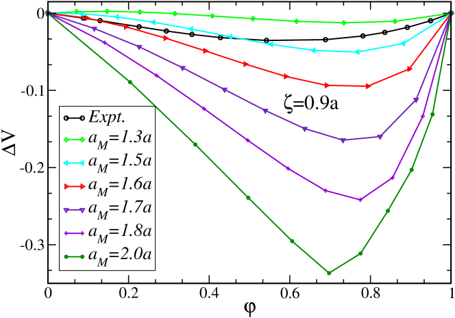
Figure 4: (color online) Dependence of the excess volume as a function of the solute volume fraction for a range of hard core diameters $a_{\rm M}$, for the dimer model with $\zeta=0.9a$. The simulations are done at $T=0.5$ and $P=0.02$. The experimental result (circles) are for $T=298$K and $P=0.1$MPa Mcglashan1976 , where the maximum volume fraction reduction occurs at $\varphi_{\rm max}\approx 59.7\%$. For the simulation results, when $a_{\rm M}\leq 1.3a$, the excess volume has both positive and negative values. As $a_{\rm M}$ increases, the excess volume becomes more negative and $\varphi_{\rm max}$, the maximum reduction volume fraction, decreases.

Because there are several parameters in our dimer model, we first investigate how these affect the simulations, searching for a set of parameters that can best model ambient methanol. Since the goal is to explore the excess properties of the model, vis a vis real methanol-water solution, we compare our simulation results with the results reported in Ref. Mcglashan1976 concerning the excess volume at $T=298$K and $P=0.1$ MPa. We set our simulation temperature and pressure at $T=0.5$ and $P=0.02$, and we change the diameter of the hard spheres that model the methyl group in methanol. In Fig. 4, we show the excess volume of the solutions with different hard core diameters of the hard spheres $a_{\rm M}$, for a fixed bond length $\zeta=0.9a$, across the entire range of amphiphilic solute volume fraction. If $a_{\rm M}\leq 1.3a$, we cannot reproduce the volume reduction over the entire range of volume fraction. If $a_{\rm M}>1.3a$, the mixture shrinks over the entire range of volume fractions. When the hard core diameter increases, the volume fraction corresponding to maximum volume reduction (henceforth referred to as maximum reduction volume fraction) decreases. However, for this value of $\zeta$ we cannot reproduce the experimentally-observed maximum reduction volume fraction.

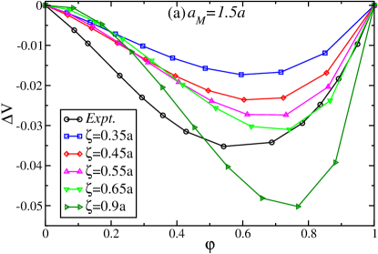
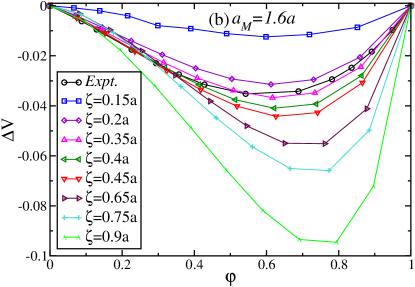
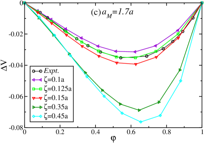
Figure 5: (color online) Dependence of the excess volume on solute volume fraction for various solute bond lengths $\zeta$ at three values of hard core diameter $a_{\rm M}$. The simulations are done at $T=0.5$ and $P=0.02$. (a) $a_{\rm M}=1.5a$, (b) $a_{\rm M}=1.6a$, (c) $a_{\rm M}=1.7a$. As $\zeta$ increases, the excess volume, $\bigtriangleup V$ becomes more negative and the maximum reduction volume fraction $\varphi_{\rm max}$ increases. Calculations performed using the parameter sets $\zeta=0.35a$, $a_{\rm M}=1.6a$ in (b) and $\zeta=0.125a$, $a_{\rm M}=1.7a$ in (c) agree well with experiment.

We next show, in Fig. 5, how bond length affects the excess volume. We choose three different hard sphere diameters and vary the bond length. For $a_{\rm M}=1.5a$ [Fig. 5(a)], as the bond length increases, the excess volume becomes more negative and the maximum reduction volume fraction increases, but its value is always larger than in experiments. For $a_{\rm M}=1.6a$ [Fig. 5(b)] and $a_{\rm M}=1.7a$ [Fig. 5(c)], the excess volume and the maximum reduction volume fraction exhibit the same trend as the bond changes as seen for $a_{\rm M}=1.5a$. However, their maximum reduction volume fraction is smaller and closer to the experimental data. Thus, we can see that the maximum reduction volume fraction $\varphi_{\rm max}$ and the corresponding $\bigtriangleup V_{\rm max}$ agree well with the experimental observations for selected bond lengths; i.e., for $a_{\rm M}=1.6a$ and $\zeta=0.35a$, $\varphi_{\rm max}=63.6\%,\bigtriangleup V_{\rm max}=-3.67\%$, and for $a_{\rm M}=1.7a$ and $\zeta=0.125a$, $\varphi_{\rm max}=58.717\%$, $\bigtriangleup V_{\rm max}=-3.55\%$. In addition, over the entire range of volume fractions the excess volume agrees quantitatively with experiment for these two sets of parameters.

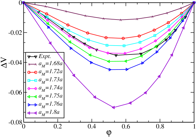
Figure 6: (color online) Dependence of the excess volume on solute volume fraction for various hard core diameter values ($a_{\rm M}$), in the monomer ($\zeta=0$) model. Simulations at $T=0.5$ and $P=0.02$. As $a_{\rm M}$ increases, $\bigtriangleup V$ becomes more negative; the maximum reduction volume fraction $\varphi_{\rm max}$ is relatively insensitive to $a_{M}$. The excess volume at $a_{\rm M}=1.74a$ is similar to experiment, but the results are less accurate than for the dimer model [see Fig. 5(b) and 5(c)].

In the dimer model, we achieve the closest agreement with the experimental data at $a_{\rm M}=1.7a$ and $\zeta=0.125a$. At this set of parameters, the hard sphere and the Jagla particle nearly overlap. The dimer model can thus be modeled as a monomer with a hard core $a_{\rm M}\approx 1.7a$, as shown in Eqs. (5) and (6). In order to achieve the closest agreement with the experimental data, we vary the single parameter, $a_{\rm M}$ in this model (Fig. 6). For all cases of $a_{\rm M}$, the reduction property can be reproduced across the entire range of volume fractions. At $a_{\rm M}=1.73a$ and $a_{\rm M}=1.75a$, the trend of the excess volume is very similar to the experimental results. For $a_{\rm M}=1.74a$, the maximum reduction volume fraction is close to the experimental data, and in the range of volume fractions smaller than the maximum reduction volume fraction, the excess volume is also quantitatively reproduced. Overall, the monomer model can reproduce the excess volume curve qualitatively but is not as accurate as the dimer model.

At $T=298$K and $P=0.1$ MPa, the methanol density is 0.78663 g/cc Mcglashan1976 , and its ratio with respect to water is 0.79. We have explored the relative density of the neat amphiphilic solutes with respect to a pure Jagla solvent when we change the parameters. The density increases when we shorten the bond length, when the diameter of the hard sphere $a_{\rm M}$ in the dimer model decreases, and when the hard core of the monomer $a_{\rm M}$ decreases. From the above-discussed results we know that when $a_{\rm M}=1.7a$ and $\zeta=0.125a$, we achieve the best agreement between our simulation results and the experimental results. However, the density ratio of the pure solute for this set of parameters is 0.66, less than the density ratio of real methanol at $T=298$ K and $P=0.1$ MPa. In the monomer model, when the hard core diameter of monomer is $a_{\rm M}=1.74a$, the density ratio is 0.64, also less than the experimental value.

III.2 Temperature and pressure dependence of the excess volume

Experimentally, when the temperature change is small, e.g., 5K, the change of the maximum reduction volume fraction is negligible and there is a small increase in $\bigtriangleup V$ as the temperature increases [Fig. 1(a)]. Over large temperature intervals, e.g., 50K, the excess volume becomes increasingly negative and the maximum reduction volume fraction increases slightly as the temperature increases [Figs. 1(b) and 1(c)]. We use our two models to check the temperature and pressure dependence of the excess volume. Choosing the parameters that can best reproduce the experimental results of the excess volume at $T=298$ K and $P=0.1$ MPa, we set $a_{\rm M}=1.7a$ and $\zeta=0.125a$ for the dimer model.

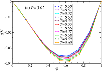
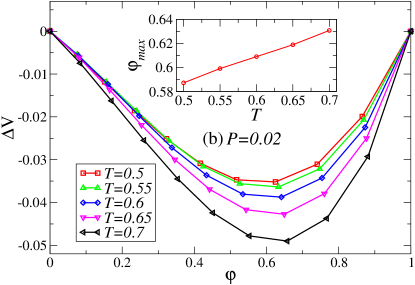
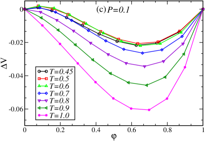
Figure 7: (color online) Dependence of the excess volume on solute volume fraction, at various temperatures and three different pressures, for the dimer model with $a_{\rm M}=1.7a$, $\zeta=0.125a$. (a) $P=0.02$, which is comparable to atmospheric pressure. The temperature difference between curves is 0.01. (b) $P=0.02$. The temperature difference between curves is 0.5. (c) $P=0.1$. As the temperature increases, the excess volume becomes more negative and the maximum reduction volume fraction increases. In (c), when the temperature is low, there is a range of dilute mixtures for which $\bigtriangleup V>0$. There are no corresponding experimental observations.

We calculate the temperature dependence of the excess volume at pressures $P=0.02$ and $P=0.1$ in the dimer model [Fig. 7]. At $P=0.02$ ($\approx 1.0$ atm), we first measure the excess volume at a series of temperatures separated by 0.01 in the range of $T=0.5$–0.6 [Fig. 7(a)]. The excess volume becomes slightly more negative and the change of the maximum reduction volume fraction is negligible as the temperature increases. When we enlarge the temperature interval to 0.05 [Fig. 7(b)], the excess volume becomes increasingly negative and the maximum reduction volume fraction increases noticeably as the temperature increases. At $P=0.1$ [Fig. 7(c)], we find approximately the same results. However, when the temperature is approximately 0.5, the excess volume of the solution with less than 15 percent of amphiphilic solutes goes to zero or becomes positive, indicating that in our model the volume does not decrease, and can even expand at these conditions. We will discuss this “bump” in the excess volume curve later. The temperature dependence at pressures $P=0.02$ and $P=0.1$ using the $a_{\rm M}=1.74a$ monomer model (not shown) are comparable to those of the dimer model.

We next compare the calculated pressure dependence of the excess volume with the experimental results. In Fig. 2, we report the experimental pressure dependence of the excess volume at two different temperatures, $T=323.15$K and $T=283.15$K, using two different pressure intervals. The results at $T=323.15$K cover pressures from $P=0.1$MPa to $P=13.5$MPa, and those at $T=283.15$K cover pressures from $P=0.1$MPa to $P=205$MPa. We can see that, as the pressure increases, the excess volume becomes less negative. Regarding the maximum reduction volume fraction of the excess volume, in Fig. 2(a), its value does not noticeably change with temperature, however in Fig. 2(b), we can clearly see that as the pressure increases, the maximum reduction volume fraction does increase.

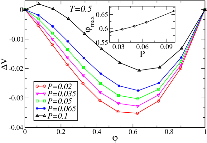
Figure 8: (color online) Dependence of the excess volume on solute volume fraction for several different pressures, at $T=0.5$, for the dimer model ($a_{\rm M}=1.7a$, $\zeta=0.125a$). As the pressure increases, the excess volume becomes more negative and the maximum reduction volume fraction increases very slightly.

In our simulation, we fix the temperature at $T=0.5$ and calculate the excess volume at pressures from $P=0.02$ to $P=0.1$. Our simulation results for the dimer model (see Fig. 8) agree with the experimental results quite well, namely, as the pressure increases the excess volume becomes less negative and the maximum reduction volume fraction increases. Regarding the positive “bump” at the small volume fraction of amphiphilic solutes, we are not aware of experimental data for this range of volume fractions, so this result is a prediction, namely that at high pressures and low temperatures, dilute methanol-water solutions have a positive excess volume. The simulation results for the best monomer model are quite similar to those for the dimer model except that the positive “bump” is smaller.

III.3 Excess enthalpy

The excess enthalpy in methanol-water solutions has been measured at $T=298$ K, and $P=0.1$ MPa LamaJCED1965 . The excess enthalpy is negative (exothermic mixing), consistent with the picture of strong association that follows from the volumetric behavior. The maximum reduction occurs at a volume fraction $\varphi_{\rm max}=42\%$, differing from that of the excess volume at these specific conditions. At pressures $P=0.1$MPa, $P=20$MPa, and $P=39$MPa, the excess enthalpy becomes less negative as the temperature increases. The maximum reduction volume fraction increases as the temperature increases. In some temperature ranges, e.g., $T=278.15$K–$T=298.15$K, the maximum reduction volume fraction actually increases as pressure increases, and the excess enthalpy becomes more negative as the pressure increases TomaszkiewiczTA1986II ; TomaszkiewiczTA1986III .

In the dimer model, when $a_{\rm M}>1.0a$, all the cases can reproduce qualitatively the enthalpy of mixing rather well. As $a_{\rm M}$ increases, the excess enthalpy becomes more negative and the maximum reduction volume fraction becomes smaller, following the same trend as in experiments. The magnitude of the excess enthalpy for $a_{\rm M}=1.7a$ and $a_{\rm M}=1.8a$ can be made close to the experimental results, but for the best model developed in Section III.A, the agreement is only qualitative.

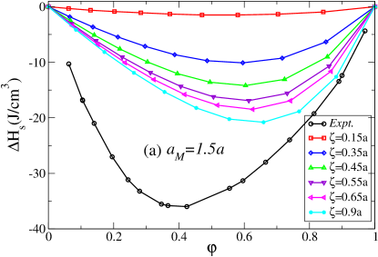
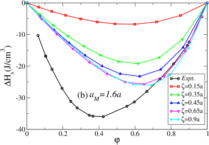
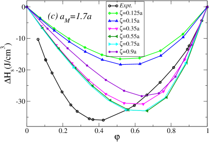
Figure 9: (color online) Dependence of the excess enthalpy on solute volume fraction for various values of the bond length, at three different hard core diameters $a_{\rm M}$, in the dimer model. The simulations are done at $P=0.02$ and $T=0.05$. (a) $a_{\rm M}=1.5a$, (b) $a_{\rm M}=1.6a$, (c) $a_{\rm M}=1.7a$. For (a) and (b), as the bond length increases, the excess enthalpy becomes more negative. For (c), the excess enthalpy exhibits a non-monotonic dependence on bond length. The maximum reduction volume fraction increases as $\zeta$ increases for all three cases.

We report the bond length dependence of the excess enthalpy at $a_{\rm HS}=1.5a$ [Fig. 9(a)], $a_{\rm M}=1.6a$ [Fig. 9(b)], and $a_{\rm M}=1.7a$ [Fig. 9(c)]. For $a_{\rm M}=1.5a$ and $a_{\rm HS}=1.6a$, as the bond length increases, the excess enthalpy becomes more negative. For $a_{\rm M}=1.7a$, the excess enthalpy first becomes more negative and then less negative as the bond length increases. For all three values of $a_{\rm M}$, the maximum reduction volume faction becomes larger as the bond length increases and the maximum enthalpy reduction is smaller than the experimental value. For the monomer model, when $a_{\rm M}>1.6a$, the excess enthalpy can also be qualitatively reproduced, and as $a_{\rm M}$ increases it becomes more negative and the maximum reduction volume fraction increases. The value of the excess enthalpy from simulations is smaller than the experimental values, but the magnitude is comparable.

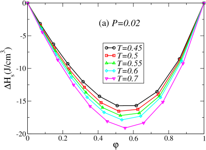
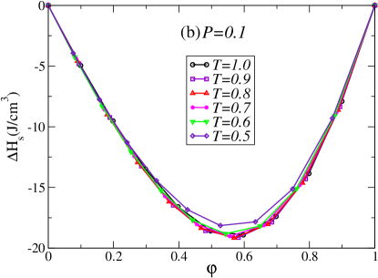
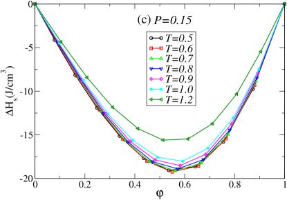
Figure 10: (color online) Dependence of the excess enthalpy on solute volume fraction for various temperatures, for the dimer model with $a_{\rm M}=1.7a$, $\zeta=0.125a$. (a) $P=0.02$. As the temperature increases, the excess enthalpy becomes more negative, in contrast to experiment, and the maximum reduction volume fraction increases TomaszkiewiczTA1986II . (b) $P=0.1$. The excess enthalpy is nearly independent of temperature. (c) $P=0.15$. When $T\geq 0.6$, the excess enthalpy decreases as the temperature increases and the volume fraction corresponding to maximum exothermicity shifts towards slightly higher values.

We return to the dimer with $a_{\rm M}=1.7a$ and $\zeta=0.125a$ and examine the temperature dependence. At $P=0.02$ [Fig. 10(a)], our simulation results contradict the experimental data: the excess enthalpy becomes increasingly negative as the temperature increases. However, the increasing maximum reduction volume fraction with increasing temperature does agree with the experimental trend. At $P=0.1$ [Fig. 10(b)], the excess enthalpy changes only very slightly with temperature, although at the highest $T$ the magnitude of the excess enthalpy decreases slightly with $T$. If we increase the pressure to $P=0.15$ [Fig. 10(c)], we can see that as the temperature increases, the magnitude of excess enthalpy decreases with $T$ and the maximum reduction volume fraction increases, in agreement with experimental trends.

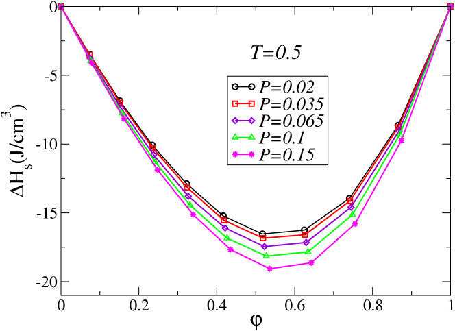
Figure 11: (color online) Dependence of the excess enthalpy on solute volume fraction for various values of the pressure, at $T=0.5$, for the dimer model with $a_{\rm M}=1.7a$, $\zeta=0.125a$. As the pressure increases, the excess enthalpy increases, and the volume fraction corresponding to maximum exothermicity increases.

In our simulation of the pressure dependence of the excess enthalpy at $T=0.5$ (Fig. 11), as the pressure increases, the excess enthalpy becomes more negative and the maximum reduction volume fraction becomes larger, which agrees well with experimental observations of methanol-water solutions.

III.4 Effect on the temperature of maximum density

At sufficiently low temperatures and pressures, the density of liquid water exhibits a maximum with respect to temperature at fixed pressure. For example, liquid water has a maximum density at $T=277$K and $P=0.1$MPa. If we add solutes to water, the temperature of the maximum density changes. According to Ref. WadaBCSJ1962 , the $T_{\rm MD}$ of a methanol solutions reaches its maximum at around $x=0.6\%$ mole fraction and then decreases slightly as the mole fraction increases, reaching 269K at $x=5\%$. This non-monotonic behavior has been explained by Chatterjee et al. using a statistical mechanical model of water DebenedettiJCP2005 .

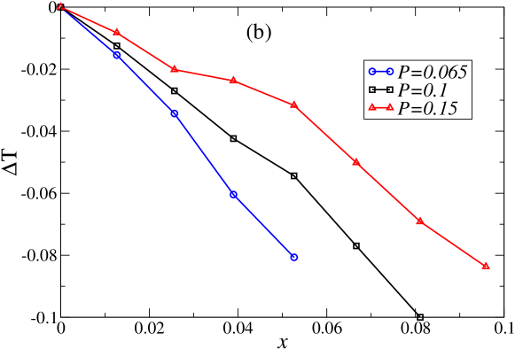
Figure 12: (color online) Effect of amphiphilic solutes on $T_{\rm MD}$ of solutions. We use the dimer with parameters of $a_{\rm M}=1.7a$, $\zeta=0.125a$. (a) The $T_{\rm MD}$ of the solutions at different solute concentrations, for $P=0.1$. (b) The shift of $T_{\rm MD}$, with respect to that of the pure solvent, $\bigtriangleup T$, as a function of solute mole fraction, $x$, at three different pressures. Note that $\bigtriangleup T$ is always negative, indicating that adding solute lowers the solution’s $T_{\rm MD}$ (lower temperatures are needed to observe negative thermal expansion). For a given mixture, the magnitude of $\bigtriangleup T$ decreases as the pressure increases.

We explore the change of the $T_{\rm MD}$ with concentration for our model. We define the change of the temperature of maximum density as $\bigtriangleup T=T_{\rm MDs}-T_{\rm MDJ}$ where $T_{\rm MDs}$ is $T_{\rm MD}$ of the solution and $T_{\rm MDJ}$ is the $T_{\rm MD}$ of the pure Jagla liquid, at the given pressure. We have carried out simulations at three different pressures for the case of dimer with $a_{\rm M}=1.7a$ and $\zeta=0.125a$. Our results are shown in Table I and Fig. 12. We find that $\bigtriangleup T$ is always negative and its absolute value increases monotonically with solute mole fraction. If we increase pressure for the same mole fraction, the change of $T_{\rm MD}$ decreases in magnitude, but it never becomes positive. Moreover, we find that the decrease of $T_{\rm MD}$ in our model is orders of magnitude stronger in methanol-water mixtures.

IV CONCLUSION

Inspired by the distinctive properties of methanol-water solutions, we construct a dimer with a hard sphere and a Jagla particle to model amphiphilic solutes. We vary the hard core diameter and the bond length to achieve the best agreement between simulations and experiment in the excess volume. We find that the best agreement occurs for the dimer with $a_{\rm M}=1.7a$ and $\zeta=0.125a$, which suggests that the dimer model can be reduced to a monomer with a large hard core and an attractive potential that coincides with the attractive part of the Jagla potential. Regarding the temperature and pressure dependence of the excess volume, our results agree qualitatively with experimental data. Our model reproduces the excess enthalpy of the methanol solutions less accurately than the excess volume. This is related to the fact that, in our simple model of amphiphilic solutes, we use the unchanged Jagla potential for the amphiphilic group. We speculate that a better agreement could be achieved if we varied the potential of the amphiphilic group. When we investigate the effect of the amphiphilic solute on the temperature of maximum density of a solution, we find that unlike in water-methanol solution, the $T_{\rm MD}$ monotonically decreases with solute concentrations. Moreover, the effect of concentration in the model is orders of magnitude stronger than in experiments.

Acknowledgments

ZS and HES thank the NSF Chemistry Division (grant CHE 0908218) for support. SVB acknowledges the partial support of this research by the Dr. Bernard W. Gamson Computational Science Center at Yeshiva College. PGD and PJR gratefully acknowledge the support of the National Science Foundation (Collaborative Research Grants CHE-0908265 and CHE-0910615). PJR also gratefully acknowledges additional support from the R. A. Welch Foundation (F-0019).

Table 1: The temperature of maximum density, $T_{\rm MD}$, and the difference between the $T_{\rm MD}$ of the solution and that of the pure solvent at the given pressure, $\bigtriangleup T$, for solutions with different mole fractions of amphiphilic solutes in Jagla solvents, at different pressures. Results are for the dimer solute model with $a_{\rm M}=1.7a$, $\zeta=0.125a$.

	P=0.065		P=0.1		P=0.15
x$\times$100	$T_{\rm MD}$	$\bigtriangleup T$	$T_{\rm MD}$	$\bigtriangleup T$	$T_{\rm MD}$	$\bigtriangleup T$
0	0.507	0	0.516	0	0.510	0
1.27	0.491	-0.016	0.504	-0.012	0.502	-0.008
2.56	0.472	-0.035	0.489	-0.027	0.490	-0.02
3.90	0.446	-0.062	0.474	-0.04	0.486	-0.024
5.26	0.426	-0.81	0.462	-0.51	0.478	-0.032
6.67	–	–	0.439	-0.77	0.46	-0.05
8.11	–	–	0.416	-0.1	0.441	-0.069
9.59	–	–	–	–	0.426	-0.0837

Figure 3: Sketch of the interaction potentials in our simulation. (a) The spherically symmetric “two-scale” Jagla ramp potential. The two length scales are the hard core diameter $r=a$, and the soft core diameter $r=b$. We study the case $U_{R}=3.56U_{0}$, $b=1.72a$ and a long range cutoff $c=3a$. (b) The interaction potential between two monomers, with contact distance $a_{\rm M}$. (c) The interaction potential between the Jagla particle and the monomer, contacting at $(a+a_{\rm M})/2$.

References

- (1) G. Akerlof, J. Am. Chem. Soc. 54, 4126 (1932).
- (2) R. E. Gibson, J. Am. Chem. Soc. 57, 1551 (1935).
- (3) H. Frank and M. Evans, J. Chem. Phys. 13, 507 (1945)
- (4) R. F. Lama and C.-Y. Lu, J. Chem. Eng. Data 10, 216 (1965).
- (5) M. L. McGlashan and A. G. Williamson, J. Chem. Eng. Data 21, 196 (1976).
- (6) G. C. Benson, and O. Kiyohara, J. Sol. Chem. 9, 791 (1980).
- (7) H. Kubota, Y. Tanaka, and T. Makita, International J. Thermophysics 9, 47 (1987).
- (8) I. Tomaszkiewicz, S. L. Randzio, and P. Gireycz, Thermochimica Acta 103, 281 (1986).
- (9) I. Tomaszkiewicz, and S. L. Randzio, Thermochimica Acta 103, 291 (1986).
- (10) C. B. Xiao, and H. Bianchi, and P. R. Tremaine, J. Chem. Therm. 29, 261 (1997).
- (11) T. Sato, A. Chiba, and R. Nozaki, J. Chem. Phys. 112, 2924 (2000).
- (12) W. L. Jorgensen, J. Phys. Chem 90, 1276 (1986).
- (13) H. J. C. Berendsen, J. R. Grigera, and T. P. Straattsma, J. Phys. Chem. 91, 6269 (1987).
- (14) W. L. Jorgensen, J. Chandrasekhar, J. D. Madura, R. W. Impey, and M. L. Klein, J. Chem. Phys. 79, 926 (1983).
- (15) W. L. Jorgensen and J. D. Madura, Mol. Phys. 56, 1381 (1985).
- (16) M. W. Mahoney and W. L. Jorgensen, J. Chem. Phys. 112, 8910 (2000).
- (17) M. Rerrario, M. Haughney, I. R. McDonald, and M. Klein, J. Chem. Phys. 93, 5156 (1990).
- (18) H. Tanaka and K. E. Gubbins, J. Chem. Phys. 97, 2626 (1992).
- (19) E. J. W. Wensink, A. C. Hoffmann, P. J. van Maaren, and D. van der Spoel, J. Chem. Phys. 119, 7308 (2003).
- (20) D. Gonzalez-Salgado and I. Nezbeda, Fluid Phase Equilibria 240, 161 (2006).
- (21) I. Bako, T. Megyes, S. Balint, T. Grosz, and V. Chihaia, Phys. Chem. Chem. Phys. 10, 5004 (2008).
- (22) Y. Zhong, G. L. Warren, and S. Patel, J. Comput. Chem. 29, 1142 (2008). (1998).
- (23) E. A. Jagla, Phys. Rev. E 63, 061501 (2001). (1999).
- (24) J. R. Errington, and P. G. Debenedetti, Nature 409, 318 (2001).
- (25) Z. Yan, S. V. Buldyrev, N. Giovambattista, and H. E. Stanley, Phys. Rev. Lett. 95, 130604 (2005).
- (26) Z. Yan, S. V. Buldyrev, N. Giovambattista, P. G. Debenedetti, and H. E. Stanley, Phys. Rev. E 73, 051204 (2006).
- (27) Z. Yan, S. V. Buldyrev, P. Kumar, N. Giovambattista, and H. E. Stanley, Phys. Rev. E 77, 042201 (2008).
- (28) L. Xu, P. Kumar, S. V. Buldyrev, S. -H. Chen, P. Poole, F. Sciortino, and H. E. Stanley, Proc. Natl. Acad. Sci. USA 102, 16807 (2005).
- (29) L. Xu, S. V. Buldyrev, C. A. Angell, and H. E. Stanley, Phys. Rev. E 74, 031108 (2006).
- (30) S. V. Buldyrev, P. Kumar, P. G. Debenedetti, P. J. Rossky, and H. E. Stanley, Proc. Natl. Acad. Sci. USA 104, 20177 (2007).
- (31) G. Wada and S. Umeda, Bull. Chem. Soc. Jpn. 35, 646 (1962).
- (32) S. Chatterjee, H. S. Ashbaugh, and P. G. Debenedetti, J. Chem. Phys. 123, 164503 (2005).