Abstract

In this proceeding we review some of our recent results for the vector meson electromagnetic form factors and structure functions in the Sakai-Sugimoto model. The latter is a string model that describes many features of the non-perturbative regime of Quantum Chromodynamics in the large $N_{c}$ limit.

1 Introduction

It was shown by ’t Hooft in 1973 [1] that considering the large $N_{c}$ limit of Quantum Chromodynamics (QCD) the amplitudes simplify and we can treat $1/N_{c}$ as a parameter for perturbative expansions. Moreover, the Feynman diagrams can be redrawn as surfaces with different topologies so that the $1/N_{c}$ expansion is interpreted as an expansion in the genus of the surfaces. The ’t Hooft approach is known as large $N_{c}$ QCD and the genus expansion is similar to the one that arises in String Theory suggesting a duality between quantum field theories and string theories.

The first concrete duality between quantum field theories and string theories was proposed by Maldacena in 1997 [2]. A careful analysis of brane embeddings in SuperString/M Theory led him to conjecture a correspondence between quantum field theories with conformal symmetry (CFT) in $D$ spacetime dimensions and Superstring/M theory compactifications on a $D+1$ Anti-de-Sitter (AdS) spacetime. The Maldacena duality, known as the AdS/CFT correspondence, relates the strong (weak) coupling regime of a quantum field theory to the weak (strong) coupling regime of a Superstring/M theory.

Inspired by the AdS/CFT correspondence, several quantum field theories that have string duals have been investigated. Of special interest is the study of string models dual to strongly coupled theories similar to QCD. This intense area of research is known as AdS/QCD (for a review see [3, 4, 5]). This is a powerful approach to non-perturbative QCD because many results do not depend on the particular string model. There is one string model, though, that has a field content very similar to large $N_{c}$ QCD in the regime of large distances and massless quarks. This is the Sakai-Sugimoto model (2004) [6] that realizes confinement and chiral symmetry breaking.

The Sakai-Sugimoto model predicts at large distances an effective four-dimensional lagrangian that includes the non-linear sigma model with a Skyrme interaction term. The latter is a very successful effective model for large $N_{c}$ QCD at large distances. On top of that, the Sakai-Sugimoto model allows the description of vector mesons which are a key ingredient in hadronic interactions. This is because of the experimentally observed vector meson dominance [7] which is the decomposition of photon-hadron interaction into vector meson exchange. All these features turn the Sakai-Sugimoto model into a good candidate for predicting scattering cross sections in non-perturbative QCD.

We review in this proceeding the calculation of vector meson electromagnetic form factors [8] and structure functions [9] in the Sakai-Sugimoto model. We begin this review recalling in section 2 the basic langauge of electromagnetic scattering of hadrons. Then we review in section 3 the Sakai-Sugimoto model and the property of vector meson dominance. In section 4 we describe the calculation of vector meson electromagnetic form factors and structure functions. For simplicity, we focus on the case where the initial state is a $\rho$ meson. We show how to extract from the Sakai-Sugimoto model a generalized electromagnetic form factor that includes elastic and non-elastic scattering. As for the structure functions, we consider only processes where one vector meson resonance is produced in the final state. We finish the review with some conclusions and perspectives of future developments.

2 Electromagnetic scattering of hadrons

Consider the electromagnetic scattering of a lepton $\ell^{-}$ with momentum $k$ and a hadron $H$ with momentum $p$ :

$$\ell^{-}(k)\,+\,H(p)\,\to\,\ell^{-}(k^{\prime})+X\,.$$ (1)

In this process the lepton and hadron exchange a virtual photon $\gamma^{*}$ with momentum $q^{\mu}\,=\,k^{\mu}-k^{\prime\mu}$. The $X$ symbol represents a hadronic final state that is (or is not ) measured when the scattering is exclusive (inclusive). We will focus on the case where $X$ represent one hadronic resonance although in general $X$ may represent two or more particles. The kinematical variables relevant for this process are

• The mass of the initial hadron :  $M=\sqrt{-p^{2}}$   ,

• The virtuality :  $q^{2}\,=\,-q_{0}^{2}+\vec{q}^{2}>0$   ,

• The Bjorken variable :  $x\,=\,-q^{2}/(2p\cdot q)$   ,

• The photon-hadron c.m. energy :  $W\,=\,\sqrt{-(p+q)^{2}}$  .

The physical region of scattering is $0<x\leq 1$ and elastic scattering corresponds to $x=1$. Note that we are working in the signature $(-,+,+,+)$.

Now consider Deep Inelastic Scattering (DIS) which is the inclusive electromagnetic scattering of a lepton and a hadron. Using the Feynman rules for the process (1), the DIS differential cross section (for the unpolarized case) can be written as

$$d^{2}\sigma\,=\,\left(\frac{1}{4ME}\right)\frac{d^{3}\vec{k}}{(2\pi)^{3}2E^{\prime}}\,\frac{e^{4}}{q^{4}}(4\pi)\,L_{\mu\nu}\,W^{\mu\nu}\,,$$ (2)

where

$$L_{\mu\nu} \,=\, \frac{1}{2}\sum_{\sigma,\sigma^{\prime}}\overline{u}(k,\sigma)\gamma_{\mu}u(k^{\prime},\sigma^{\prime})\,\overline{u}(k^{\prime},\sigma^{\prime})\gamma_{\nu}u(k,\sigma)\,,$$ (3)

$$W^{\mu\nu} \,=\, \frac{1}{4\pi(2s_{H}+1)}\sum_{\sigma_{H}}\sum_{X}(2\pi)^{4}\delta^{4}(p+q-p_{X})\langle p,\sigma_{H}|J^{\mu}(0)|X\rangle$$ (4)

$$\times \langle X|J^{\nu}(0)|p,\sigma_{H}\rangle\,.$$ (5)

The tensor $L_{\mu\nu}$ carries the information of the initial and final leptons (leptonic tensor) while the tensor $W^{\mu\nu}$ describes the response of a hadron H to an electromagnetic current $J^{\nu}(x)$ (hadronic tensor). Using current conservation and relevant QCD symmetries like parity, time reversal and Lorentz invariance we can decompose the hadronic tensor as

$$W^{\mu\nu}=F_{1}(x,q^{2})\Big{(}\eta^{\mu\nu}-\frac{q^{\mu}q^{\nu}}{q^{2}}\Big{)}\,+\,\frac{2x}{q^{2}}F_{2}(x,q^{2})\Big{(}p^{\mu}+\frac{q^{\mu}}{2x}\Big{)}\Big{(}p^{\nu}\,+\,\frac{q^{\nu}}{2x}\,\Big{)}\,,$$ (6)

where $F_{1}(x,q^{2})$ and $F_{2}(x,q^{2})$ are known as the structure functions of the hadron.

In the hadronic tensor each final state $X$ contributes through the current matrix element $\langle p,\sigma_{H}|J^{\mu}_{H}(0)|X\rangle$. In the case where the final state is one hadron with the same quantum numbers as the initial hadron but a different mass the current matrix element can be decomposed as

$$\langle p,n,\sigma_{H}|J^{\mu}(0)|p+q,n_{X},\sigma_{X}\rangle\,=\,\sum_{i}\Gamma_{i}^{\mu}(p,q)\,F^{i}_{n,n_{X}}(q^{2})\,,$$ (7)

where $n$ ($n_{X}$) is an index associated to the mass of the initial (final) hadron. The functions $F^{i}_{n,n_{X}}(q^{2})$ are the generalized electromagnetic form factors that include the elastic ($n=n_{X}$) and transition ($n\neq n_{X}$) form factors.

As a example, let’s consider the elastic $\rho$ meson form factor where $n_{X}=n=1$. In that case the current can be decomposed as

$$\langle p,\epsilon|J^{\mu}(0)|p+q,\epsilon^{\prime}\rangle = \epsilon\cdot\epsilon^{\prime}(2p+q)^{\mu}F_{1}(q^{2})+\left[\epsilon^{\mu}\epsilon^{\prime}\cdot q-{\epsilon^{\prime}}^{\mu}\epsilon\cdot q\right]\Big{[}F_{1}(q^{2})$$ (8)

$$+ F_{2}(q^{2})\Big{]}-\frac{q\cdot\epsilon^{\prime}q\cdot\epsilon}{M^{2}}(2p+q)^{\mu}F_{3}(q^{2})\,.$$ (9)

3 The Sakai-Sugimoto model

In the regime of low momentum transfer ($\sqrt{q^{2}}$ lower than some $GeVs$), soft (non-perturbative) processes become dominant in hadronic scattering. Lattice QCD (the numerical approach of substituting the continuous spacetime by a lattice of points) is not very useful here because of time dependence in scattering processes. Effective models are very useful but they don’t succeed completely when comparing with experimental results. As stressed in the introduction, the Sakai-Sugimoto model provides a new insight into the problem of hadronic scattering in the non-perturbative regime. This model consists in the introduction of $N_{f}$ D8-$\overline{\mbox{D~{}\,}}\!\!\!$8 branes into a set of $N_{c}$ D4 branes in the limit of large $N_{c}$ with fixed $N_{f}$. This limit allows a supergravity description and can be interpreted as the quenching limit in QCD. The Sakai-Sugimoto model is the first string model that realizes confinement and chiral symmetry breaking. Below we describe this model in some detail.

Consider a set of $N_{c}$ coincident D4-branes with a compact spatial direction in type IIA Supergravity [10]. They generate a background composed by a metric, dilaton and four-form :

$$ds^{2} = \frac{u^{\scriptscriptstyle 3/2}}{R^{\scriptscriptstyle 3/2}}\left[\eta_{\mu\nu}dx^{\mu}dx^{\nu}+f(u)d\tau^{2}\right]+\frac{R^{\scriptscriptstyle 3/2}}{u^{\scriptscriptstyle 3/2}}\frac{du^{2}}{f(u)}+R^{\scriptscriptstyle 3/2}u^{\scriptscriptstyle 1/2}d\Omega_{4}^{2}\,,$$ (10)

$$f(u) = 1-\frac{u_{\Lambda}^{3}}{u^{3}}\quad,\quad e^{\phi}=g_{s}\frac{u^{3/4}}{R^{3/4}}\quad,\quad F_{4}=\frac{(2\pi l_{s})^{3}N_{c}}{V_{\scriptscriptstyle S^{4}}}\epsilon_{4}\,,$$ (11)

where $R=(\pi g_{s}N_{c})^{1/3}\sqrt{\alpha^{\prime}}$. The $\tau$ coordinate is compact with period

$$\delta\tau=\frac{4\pi}{3}\frac{R^{3/2}}{u_{\Lambda}^{1/2}}\equiv\frac{2\pi}{M_{\Lambda}}\,,$$ (12)

where $M_{\Lambda}$ is a 4-d mass scale. This compactification is introduced as a mechanism of supersymmetry breaking and confinement. Imposing anti-periodic conditions for the fermionic states we get at low energies a four-dimensional non-supersymmetric strongly coupled $U(N_{c})$ theory at large $N_{c}$ with ’t Hooft constant given by

$$\lambda=g_{YM}^{2}N_{c}=(2\pi M_{\Lambda})\,g_{s}N_{c}\,l_{s}\,.$$ (13)

It is convenient to introduce use a pair of dimensionless coordinates $y$ and $z$ defined by the relations

$$u=u_{\Lambda}\left(1+y^{2}+z^{2}\right)^{1/3}\equiv u_{\Lambda}K_{y,z}^{1/3}\quad,\quad\tau=\frac{\delta\tau}{2\pi}\arctan\left(\frac{z}{y}\right)\,.$$ (14)

In terms of these coordinates the metric takes the form

$${\rm d}s^{2} = u_{\Lambda}^{3/2}R^{-3/2}K_{y,z}^{1/2}\,\eta_{\mu\nu}{\rm d}x^{\mu}{\rm d}x^{\nu}\,+\,\frac{4}{9}R^{3/2}u_{\Lambda}^{1/2}\frac{K_{y,z}^{-5/6}}{y^{2}+z^{2}}\Big{[}(z^{2}+y^{2}K_{y,z}^{1/3}){\rm d}z^{2}$$ (15)

$$+ (y^{2}+z^{2}K_{y,z}^{1/3}){\rm d}y^{2}+2yz(1-K_{y,z}^{1/3}){\rm d}y{\rm d}z\Big{]}+R^{3/2}U_{\scriptscriptstyle KK}^{1/2}K_{y,z}^{1/6}{\rm d}\Omega_{4}^{2}\,.$$ (16)

Now consider $N_{f}$ coincident D8-$\overline{\mbox{D~{}\,}}\!\!\!$8 probe branes living in the background generated by the $N_{c}$ D4-branes. The probe approximation is guaranteed by the condition $N_{f}\ll N_{c}$. The $N_{f}$ D8 branes bring quark degrees of freedom as fundamental strings extending from the D4 branes to the D8 branes. The dynamic of the D8 and $\overline{\mbox{D~{}\,}}\!\!\!$8 branes is dictated by the DBI action. It turns out that the solution to the DBI equations merge the D8 and $\overline{\mbox{D~{}\,}}\!\!\!$8 branes in the infrared region (small $u$). This is a geometrical realization of chiral symmetry breaking $U(N_{f})\times U(N_{f})\to U(N_{f})$. In the simplest case the solution is just $y=0$ (antipodal solution) and the induced D8-$\overline{\mbox{D~{}\,}}\!\!\!$8 metric takes the format

$${\rm d}s_{D8} = u_{\Lambda}^{3/2}R^{-3/2}K_{z}^{1/2}\,\eta_{\mu\nu}{\rm d}x^{\mu}{\rm d}x^{\nu}\,+\,\frac{4}{9}R^{3/2}u_{\Lambda}^{1/2}K_{z}^{-5/6}{\rm d}z^{2}$$ (17)

$$+ R^{3/2}u_{\Lambda}^{1/2}K_{z}^{1/6}{\rm d}\Omega_{4}^{2}\,,$$ (18)

where $K_{z}=1+z^{2}$. Using the DBI action we can describe 9-d gauge field fluctuations in the D8-$\overline{\mbox{D~{}\,}}\!\!\!$8 branes. Considering small gauge field fluctuations $A_{\mu},A_{z}$ depending only in $x^{\mu}$ and $z$ directions the DBI action reduces to a Yang-Mills action that can be integrated in $S^{4}$ leading to

$$S_{YM}=-\kappa\int d^{4}xdz{\rm Tr}\left[\frac{1}{2}K_{z}^{-1/3}\eta^{\mu\rho}\eta^{\nu\sigma}F_{\mu\nu}F_{\rho\sigma}+M_{\Lambda}^{2}\,K_{z}\eta^{\mu\nu}F_{\mu z}F_{\nu z}\right]$$ (19)

where $\kappa=\lambda N_{c}/(216\pi^{3})$. The gauge field $A_{\mu}$ can be expanded, in the $A_{z}=0$ gauge, as

$$A_{\mu}(x,z)=\hat{\cal V}_{\mu}(x)+\hat{\cal A}_{\mu}(x)\psi_{0}(z)+\sum_{n=1}^{\infty}\left[v_{\mu}^{n}(x)\psi_{2n-1}(z)+a_{\mu}^{n}(x)\psi_{2n}(z)\right]$$ (20)

where

$$\hat{\cal V}_{\mu}(x) = \frac{1}{2}U^{-1}\left[{\cal A}^{L}_{\mu}+\partial_{\mu}\right]U+\frac{1}{2}U\left[{\cal A}^{R}_{\mu}+\partial_{\mu}\right]U^{-1}\,,$$ (21)

$$\hat{\cal A}_{\mu}(x) = \frac{1}{2}U^{-1}\left[{\cal A}^{L}_{\mu}+\partial_{\mu}\right]U-\frac{1}{2}U\left[{\cal A}^{R}_{\mu}+\partial_{\mu}\right]U^{-1}\,,$$ (22)

$$U(x) = e^{\frac{i\pi(x)}{f_{\pi}}}\quad,\quad{\cal A}^{L(R)}_{\mu}(x)={\cal V}_{\mu}(x)\pm{\cal A}_{\mu}(x)\,,$$ (23)

and the $\psi_{n}(z)$ modes satisfy

$$\kappa\int dz\,K_{z}^{-1/3}\psi_{n}(z)\psi_{m}(z)=\delta_{nm}\quad,\quad-K_{z}^{1/3}\partial_{z}\left[K_{z}\partial_{z}\psi_{n}(z)\right]=\lambda_{n}\,\psi_{n}(z)\,.$$ (24)

Using the Kaluza-Klein expansion (20) and integrating the $z$ coordinate we get a four-dimensional effective lagrangian of mesons and external $U(1)$ fields. The vector (axial vector) mesons are represented by the fields $v_{\mu}^{n}(x)$ ($a_{\mu}^{n}(x)$) and correspond to the modes $\psi_{2n-1}(z)$ ($\psi_{2n}(z)$). The pion is represented by the field $\pi(x)$ and corresponds to the mode $\psi_{0}(z)$. In addition, we have external $U(1)$ vector (axial) fields represented by ${\cal V}_{\mu}$ (${\cal A}_{\mu}$).

In order to have a diagonal kinetic term, the vector mesons are redefined as $\tilde{v}_{\mu}^{n}=v_{\mu}^{n}+(g_{v^{n}}/M_{v^{n}}^{2}){\cal V}_{\mu}$ and the quadratic terms in the vector sector take the form [11] :

$${\cal L}_{2} = \frac{1}{2}\sum_{n}\left[{\rm Tr}\left(\partial_{\mu}\tilde{v}_{\nu}^{n}-\partial_{\nu}\tilde{v}_{\mu}^{n}\right)^{2}+2M_{v^{n}}^{2}{\rm Tr}\left(\tilde{v}_{\mu}^{n}-\frac{g_{v^{n}}}{M_{v^{n}}^{2}}{\cal V}_{\mu}\right)^{2}\right]\,,$$

where

$$M_{v^{n}}^{2}=\lambda_{\scriptscriptstyle 2n-1}M^{2}_{\Lambda}\quad,\quad g_{v^{n}}=\kappa\,M_{v^{n}}^{2}\int dz\,K_{z}^{-1/3}\psi_{\scriptscriptstyle 2n-1}(z)\,.$$

The mixed term $g_{v^{n}}\tilde{v}_{\mu}^{n}{\cal V}^{\mu}$ represents the decay of the photon into vector mesons which is a holographic realization of vector meson dominance.

4 Form factors and structure functions of vector mesons in the Sakai-Sugimoto model

In section 2 we described how the hadronic structure functions and form factors arise in the electromagnetic scattering of hadrons. The hadronic structure functions describe the inclusive interaction between a virtual photon and a hadron (Deep Inelastic Scattering). They carry information of the partonic structure of hadron through the parton distribution functions. The latter are probability densities that describe how the partons (valence quarks, gluons and sea quark-antiquark pairs) distribute inside a hadron along the longitudinal momentum. The electromagnetic form factors of hadrons describe the exclusive interaction between a photon and two hadrons. In the elastic case these quantities give information about the distribution of charge and magnetic moment inside a hadron. In the non-elastic case they describe the transition between different hadronic states and are usually written in terms of helicity amplitudes. Below we describe how to calculate electromagnetic form factors and structure functions of vector mesons in the Sakai-Sugimoto model.

4.1 Electromagnetic form factors

Electromagnetic form factors of vector mesons have been obtained previously using holographic bottom-up (phenomenological) models [12, 13] as well as top-down string models dual to supersymmetric field theories [14, 15]. Below we review the calculation of vector meson electromagnetic form factors in the Sakai-Sugimoto model [8] .

From the cubic terms in the 4-d effective meson lagrangian discussed in the previous section we can extract the vector meson interaction term

$${\cal L}_{vvv} = \sum_{n,\ell,m}g_{v^{n}v^{\ell}v^{m}}{\rm Tr}\Big{\{}\left(\partial^{\mu}{\tilde{v}}^{\nu\,n}-\partial^{\nu}{\tilde{v}}^{\mu\,n}\right)[{\tilde{v}}_{\mu}^{\ell},{\tilde{v}}_{\nu}^{m}]\Big{\}}$$ (25)

where $g_{v^{n}v^{\ell}v^{m}}$ are 4-d effective couplings given by the integral

$$g_{v^{n}v^{\ell}v^{m}}=\kappa\,\int dz\,K_{z}^{-1/3}\psi_{2n-1}(z)\psi_{2\ell-1}(z)\psi_{2m-1}(z)\,.$$ (26)

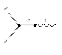
Figure 1: Exclusive scattering of a photon and two vector mesons

Now consider the exclusive scaterring of a photon with two vector mesons $v^{m}$ and $v^{\ell}$ as described in Figure 1. The photon decays into a vector meson $v^{n}$ that propagates and interact with the external vector mesons. Using the Feynman rules associated to this process we find the electromagnetic current matrix element for vector mesons states :

$$\langle v^{m}(p),\epsilon|J^{\mu}(0)|v^{\ell}(p+q),\epsilon^{\prime}\rangle=\left[\sum_{n=1}^{\infty}{g_{v^{n}}g_{v^{m}v^{n}v^{\ell}}}\Delta^{\mu\sigma}(q,m_{n}^{2})\right]$$ (27)

$$\epsilon^{\nu}{\epsilon^{\prime}}^{\rho}\Big{[}\eta_{\sigma\nu}(q-p)_{\rho}+\eta_{\nu\rho}(2p+q)_{\sigma}-\eta_{\rho\sigma}(p+2q)_{\nu}\Big{]}$$ (28)

where $\Delta^{\mu\sigma}(q,m_{n}^{2})$ is the propagator of a massive vector particle with momentum $q$ and mass $m_{n}^{2}$. Using the holographic sum rule

$$\sum_{n=1}^{\infty}\frac{g_{v^{n}}g_{v^{n}v^{m}v^{\ell}}}{M_{v^{n}}^{2}}=\delta_{m\ell}$$ (29)

and the transversality of the initial and final polarizations we get the simple expression

$$\langle v^{m}(p),\epsilon|J^{\mu}(0)|v^{\ell}(p+q),\epsilon^{\prime}\rangle = \epsilon^{\nu}{\epsilon^{\prime}}^{\rho}\Big{[}\eta_{\nu\rho}(2p+q)_{\sigma}+2(\eta_{\sigma\nu}q_{\rho}-\eta_{\rho\sigma}q_{\nu})\Big{]}$$ (30)

$$\times \left({\eta^{\mu\sigma}-\frac{q^{\mu}q^{\sigma}}{q^{2}}}\right){\cal F}_{v^{m}v^{\ell}}(q^{2})\,,$$ (31)

where

$${\cal F}_{v^{m}v^{\ell}}(q^{2})=\sum_{n=1}^{\infty}\frac{g_{v^{n}}g_{v^{n}v^{m}v^{\ell}}}{q^{2}+M_{v^{n}}^{2}}$$ (32)

is the generalized vector meson form factor. The elastic $\rho$ meson form factors can be extracted from the case $m=\ell=1$ :

$$\langle v^{1}(p),\epsilon|J^{\mu}(0)|v^{1}(p+q),\epsilon^{\prime}\rangle = \Big{\{}(\epsilon\cdot\epsilon^{\prime})(2p+q)^{\mu}$$ (33)

$$+ 2\left[\epsilon^{\mu}(\epsilon^{\prime}\cdot q)-{\epsilon^{\prime}}^{\mu}(\epsilon\cdot q)\right]\Big{\}}{\cal F}_{v^{1}v^{1}}(q^{2})\,,$$ (34)

Comparing this result with the expansion (9) we find the $\rho$ meson form factors:

$$F_{1}(q^{2})=F_{2}(q^{2})={\cal F}_{v^{1}v^{1}}(q^{2})\,\,,\,\,F_{3}(q^{2})=0\,.$$ (35)

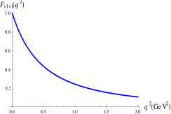
Figure 2: The $\rho$ meson form factor in the Sakai-Sugimoto model.

In Figure 2 we plot the $\rho$ meson form factor ${\cal F}_{v^{1}v^{1}}(q^{2})$. The form factor begins at ${\cal F}_{v^{1}v^{1}}(0)=1$ (as expected from charge normalization) and decreases approximately as $q^{-4}$ for large $q^{2}$ in accordance with other non-perturbative approaches to QCD (see for instance [18]) .

In order to extract some static properties of the $\rho$ meson it is useful to define the electric, magnetic, and quadrupole form factors as

$$G_{E}=F_{1}-\frac{q^{2}}{6M^{2}}\Big{[}F_{2}-(1+\frac{q^{2}}{4M^{2}})F_{3}\Big{]}\quad,\quad G_{M}=F_{1}+F_{2}\,,$$ (36)

$$G_{Q}=-F_{2}+\left(1+\frac{q^{2}}{4M^{2}}\right)F_{3}\,.$$ (37)

In the Sakai-Sugimoto model and for the $\rho$ meson they take the form

$$G_{E}=(1+\frac{q^{2}}{6M^{2}})F_{1}\quad,\quad G_{M}=2F_{1}\quad,\quad G_{Q}=-F_{1}\,.$$ (38)

From these form factors, we can extract the $\rho$ meson electric radius

$$\langle r^{2}_{\rho}\rangle=-6\frac{\mathrm{d}}{\mathrm{d}q^{2}}G_{E}(q^{2})|_{q^{2}=0}=0.5739\,,$$ (39)

and the magnetic and quadrupole moments

$$\mu=\frac{1}{2M}G_{M}(q^{2})|_{q^{2}=0}=\frac{1}{M}\quad,\quad D\,\equiv\,\frac{1}{M^{2}}G_{Q}(q^{2})|_{q^{2}=0}=-\frac{1}{M^{2}}\;.$$ (40)

4.2 Structure functions

Deep Inelastic Scattering in AdS/QCD was first investigated in a bottom-up model for the case of scalar particles [19]. Further development in bottom-up and top-down models include the large $x$ regime [20, 21, 22, 23, 24] as well as the small $x$ regime where Pomeron exchange dominates [25, 26, 27, 28, 29, 30]. Here we review the calculation of structure functions in the Sakai-Sugimoto model for the case where the initial state is a $\rho$ meson and the final state is one vector meson resonance [9].

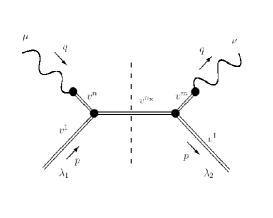
Figure 3: Diagram for a tree level contribution to Compton forward scattering

The optical theorem relates the hadronic tensor to the imaginary part of the tensor associated to the Compton forward scattering. Using the Feynman rules corresponding to the diagram of Figure 3 and the polarization vector identity

$$\sum_{\epsilon}\epsilon^{\lambda_{1}}\epsilon^{\lambda_{2}}=\eta^{\lambda_{1}\lambda_{2}}+\frac{p^{\lambda_{1}}p^{\lambda_{2}}}{M_{v^{1}}^{2}}\,,$$ (41)

we obtain

$${\rm Im}T^{\mu\nu} = \frac{N_{f}}{3}\left[\eta^{\mu\sigma_{1}}-\frac{q^{\mu}q^{\sigma_{1}}}{q^{2}}\right]\left[\eta^{\nu\sigma_{2}}-\frac{q^{\nu}q^{\sigma_{2}}}{q^{2}}\right]$$ (42)

$$\times \left[\eta^{\lambda_{1}\lambda_{2}}+\frac{p^{\lambda_{1}}p^{\lambda_{2}}}{M_{v^{1}}^{2}}\right]\left[\eta^{\rho_{1}\rho_{2}}+\frac{(p+q)^{\rho_{1}}(p+q)^{\rho_{2}}}{W^{2}}\right]$$ (44)

$$\times \left[\eta_{\sigma_{1}\lambda_{1}}(2q)_{\rho_{1}}+\eta_{\lambda_{1}\rho_{1}}(2p)_{\sigma_{1}}+\eta_{\sigma_{1}\rho_{1}}(-2q)_{\lambda_{1}}\right]$$ (45)

$$\times \left[\eta_{\sigma_{2}\lambda_{2}}(2q)_{\rho_{2}}+\eta_{\lambda_{2}\rho_{2}}(2p)_{\sigma_{2}}+\eta_{\sigma_{2}\rho_{2}}(-2q)_{\lambda_{2}}\right]$$ (46)

$$\times \sum_{n_{\bf x}}\left[{\cal F}_{v^{1}v^{n_{\bf x}}}(q^{2})\right]^{2}(2\pi)\delta[M_{v^{n_{x}}}^{2}-W^{2}]\,,$$ (47)

where ${\cal F}_{v^{1}v^{n_{\bf x}}}(q^{2})$ is given in eq.(32). We can approximate the sum over the delta functions by an integral

$$\sum_{n_{\bf x}}\delta[M_{v^{n_{x}}}^{2}-W^{2}] \equiv \sum_{n_{x}}\delta[M_{v^{n_{x}}}^{2}-M_{v^{\overline{n}}}^{2}]=\int dn_{x}\left[\left|\frac{\partial M_{v^{n_{x}}}^{2}}{\partial n_{x}}\right|\right]^{-1}\delta(n_{x}-\overline{n})$$ (48)

$$\equiv f(\overline{n})\,.$$ (49)

The structure functions, defined in eq.(6), take the form

$$F_{1}(x,q^{2}) = \frac{4N_{f}}{3}f(\overline{n})\Big{[}{\cal F}_{v^{1}v^{\overline{n}}}(q^{2})\Big{]}^{2}q^{2}\left[2+\frac{q^{2}}{4x^{2}M_{v^{1}}^{2}}+\frac{q^{2}}{W^{2}x^{2}}(x-\frac{1}{2})^{2}\right]$$ (50)

$$F_{2}(x,q^{2}) = \frac{4N_{f}}{3}f(\overline{n})\Big{[}{\cal F}_{v^{1}v^{\overline{n}}}(q^{2})\Big{]}^{2}\frac{q^{2}}{2x}\left[3+\frac{q^{2}}{M_{v^{1}}^{2}}+\frac{(q^{2})^{2}}{M_{v^{1}}^{2}W^{2}x^{2}}(x-\frac{1}{2})^{2}\right]\,.$$ (51)

In figures 4 and 5 we show the numerical results of the $\rho$ meson structure functions in the Sakai-Sugimoto model for $N_{f}=1$. The plots show $F_{1}$ and $F_{2}$ as a function of the virtuality $q^{2}$ and the Bjorken variable $x$. As expected the structure functions go to zero as $q^{2}$ goes to zero. Interestingly, the $x$ dependence of the structure functions suggest a valence quark behaviour and near $x=0.5$ we find an approximate Callan-Gross relation $F_{2}\approx 2xF_{1}$. However, in the approximation that we have considered here where the final state is composed by (only) one vector meson resonance the structure functions are very small. Further corrections may involve working with higher spin particles and $1/N_{c}$ corrections. These issues will be investigated in future works.

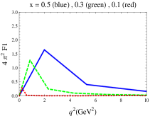
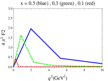
Figure 4: Structure functions as a function of the virtuality $q^{2}$

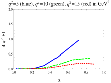
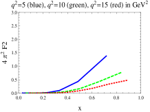
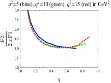
Figure 5: Structure functions as a function of the Bjorken variable $x$

5 Conclusions

The Sakai-Sugimoto model offers a new approach for the non-perturbative regime of hadronic interactions. In particular, it realizes in a simple way the property of vector meson dominance. In this proceeding we reviewed the calculation of electromagnetic form factors and structure functions of vector mesons in this model. We considered only processes where one particle is produced in the final state. Processes involving two or more particle states arise as corrections of order $1/N_{c}$ and will be the subject of future research.

The perturbative QCD approach to hadron scattering involves factorization between hard parton scattering and soft parton distribution functions. It would be interesting to understand this factorization in the AdS/QCD approach. Recently interesting models in AdS/QCD have been proposed to study the regime of high energies ($x\ll 1$) but low momentum transfer ($q^{2}\ll\Lambda$) where the soft pomeron is relevant. To develop these models in the context of the Sakai-Sugimoto model is another direction of future research.

Acknowledgment: Talk presented by C.A.B.B. at the Eleventh Workshop on Non-Perturbative Quantum Chromodynamics, Paris, June 6-10, 2011 (eConf C1106064). He thanks the organizers for the hospitality and the stimulating atmosphere. This work was sponsored by the STFC Rolling Grant ST/G000433/1 (United Kingdom) and the grants from CNPq, Capes and Faperj (Brazil).

References

- [1] G. ’t Hooft, Nucl. Phys. B72, 461 (1974).
- [2] J. M. Maldacena, Adv. Theor. Math. Phys. 2, 231 (1998) [Int. J. Theor. Phys. 38, 1113 (1999)] [arXiv:hep-th/9711200].
- [3] K. Peeters, M. Zamaklar, Eur. Phys. J. ST 152, 113-138 (2007). [arXiv:0708.1502 [hep-ph]].
- [4] J. Erdmenger, N. Evans, I. Kirsch, E. Threlfall, Eur. Phys. J. A35, 81-133 (2008). [arXiv:0711.4467 [hep-th]].
- [5] S. S. Gubser, A. Karch, Ann. Rev. Nucl. Part. Sci. 59, 145-168 (2009).
- [6] T. Sakai and S. Sugimoto, Prog. Theor. Phys. 113, 843 (2005) [arXiv:hep-th/0412141].
- [7] J. J. Sakurai, Currents and Mesons, (University of Chicago Press, Chicago, 1969)
- [8] C. A. Ballon Bayona, H. Boschi-Filho, N. R. F. Braga, M. A. C. Torres, JHEP 1001, 052 (2010). [arXiv:0911.0023 [hep-th]].
- [9] C. A. Ballon Bayona, H. Boschi-Filho, N. R. F. Braga, M. A. C. Torres, JHEP 1010, 055 (2010). [arXiv:1007.2448 [hep-th]].
- [10] E. Witten, Adv. Theor. Math. Phys. 2, 505-532 (1998). [hep-th/9803131].
- [11] T. Sakai, S. Sugimoto, Prog. Theor. Phys. 114, 1083-1118 (2005). [hep-th/0507073].
- [12] H. R. Grigoryan, A. V. Radyushkin, Phys. Lett. B650, 421-427 (2007). [hep-ph/0703069].
- [13] H. R. Grigoryan, A. V. Radyushkin, Phys. Rev. D76, 095007 (2007). [arXiv:0706.1543 [hep-ph]].
- [14] S. Hong, S. Yoon, M. J. Strassler, JHEP 0404, 046 (2004). [hep-th/0312071].
- [15] D. Rodriguez-Gomez, J. Ward, JHEP 0809, 103 (2008). [arXiv:0803.3475 [hep-th]].
- [16] C. A. B. Bayona, H. Boschi-Filho, M. Ihl, M. A. C. Torres, JHEP 1008, 122 (2010). [arXiv:1006.2363 [hep-th]].
- [17] S. Kuperstein, J. Sonnenschein, JHEP 0809, 012 (2008). [arXiv:0807.2897 [hep-th]].
- [18] B. L. Ioffe, A. V. Smilga, Nucl. Phys. B216, 373 (1983).
- [19] J. Polchinski, M. J. Strassler, JHEP 0305, 012 (2003). [hep-th/0209211].
- [20] C. A. Ballon Bayona, H. Boschi-Filho, N. R. F. Braga, JHEP 0803, 064 (2008). [arXiv:0711.0221 [hep-th]].
- [21] C. A. Ballon Bayona, H. Boschi-Filho, N. R. F. Braga, JHEP 0809, 114 (2008). [arXiv:0807.1917 [hep-th]].
- [22] B. Pire, C. Roiesnel, L. Szymanowski, S. Wallon, Phys. Lett. B670, 84-90 (2008). [arXiv:0805.4346 [hep-ph]].
- [23] C. A. B. Bayona, H. Boschi-Filho, N. R. F. Braga, M. Ihl and M. A. C. Torres, arXiv:1112.1439 [hep-ph].
- [24] E. Koile, S. Macaluso and M. Schvellinger, JHEP 1202, 103 (2012) [arXiv:1112.1459 [hep-th]].
- [25] R. C. Brower, J. Polchinski, M. J. Strassler, C. -ITan, JHEP 0712, 005 (2007). [hep-th/0603115].
- [26] Y. Hatta, E. Iancu, A. H. Mueller, JHEP 0801, 026 (2008). [arXiv:0710.2148 [hep-th]].
- [27] C. A. Ballon Bayona, H. Boschi-Filho, N. R. F. Braga, JHEP 0810, 088 (2008). [arXiv:0712.3530 [hep-th]].
- [28] L. Cornalba and M. S. Costa, Phys. Rev. D 78, 096010 (2008) [arXiv:0804.1562 [hep-ph]].
- [29] L. Cornalba, M. S. Costa, J. Penedones, JHEP 1003, 133 (2010). [arXiv:0911.0043 [hep-th]].
- [30] R. C. Brower, M. Djuric, I. Sarcevic, C. -ITan, JHEP 1011, 051 (2010). [arXiv:1007.2259 [hep-ph]].