Nonadiabatic pumping in classical and quantum chaotic scatterers

Abstract

We study directed transport in periodically forced scattering systems in the regime of fast and strong driving where the dynamics is mixed to chaotic and adiabatic approximations do not apply. The model employed is a square potential well undergoing lateral oscillations, alternatively as two- or single-parameter driving. Mechanisms of directed transport are analyzed in terms of asymmetric irregular scattering processes. Quantizing the system in the framework of Floquet scattering theory, we calculate directed currents on basis of transmission and reflection probabilities obtained by numerical wavepacket scattering. We observe classical as well as quantum transport beyond linear response, manifest in particular in a non-zero current for single-parameter driving where according to adiabatic theory, it should vanish identically.

1 Introduction

The concept of pumping in nanosystems [1] has emerged from the paradigm of peristaltic pumps, simple idealized devices moving mass and/or charge in a defined direction as two or more parameters are cycled through a closed path [2]. As long as the driving is considered slow, adiabatic approximations apply. This enormously fruitful idea allows for a very general analytical treatment involving quantum scattering theory and Berry phases [3, 4, 5, 6] and has inspired a wide range of experimental realizations, including semiconductor nanostructures, e.g., quantum dots driven by time-dependent gate voltages [7, 8] and more recently graphene sheets [9, 10]. Stimulated in turn by these developments, theoretical approaches have been extended towards quantum pumps with fast and strong driving, leaving the adiabatic regime—largely equivalent to linear response [6]—far behind [11, 12, 13, 14, 15], as well as towards including realistic many-body effects like dissipation and charge blocking.

By contrast, aspects of complex dynamics involved in directed transport in strongly driven pumps have not yet been explored in depth. From the point of view of ballistic classical motion, peristaltic pumping amounts to a trivial dynamics of the transported particles, moving phase-space volumes through the device much like a viscous liquid [4, 6, 16, 17]. As sufficiently coherent and controllable sources of ever faster drivings approaching the THz regime [18] become available, pumping in the realm of nonadiabatic and strongly nonlinear dynamics comes within reach. Scattering theory, already at the heart of quantum pumping, provides us with an appropriate theoretical framework which has developed far beyond the adiabatic regime: Irregular scattering [19] is a mature field with numerous applications from celestial mechanics [20] down to chemical reactions [21, 22, 23], comprising classical as well as quantum phenomena and approaches.

With this work, we attempt a first survey into pumps operating in the regime of chaotic scattering and to give an overview of their principal features. As concerns implications for directed transport of the nonlinear dynamics induced by fast and strong forcing, there exists a pertinent case to be followed: The concept of chaotic ratchets [24], in particular classical Hamiltonian ones amenable to direct quantization [25, 26], has stimulated important insights into conditions and mechanisms of directed transport and its quantum manifestations in this regime. Similarly, based on a comparable body of results available on scattering at strongly driven potentials [27, 28], we will point out peculiarities of pumping due to a complex dynamics, such as currents violating linear response [29] and the possibility to achieve transport with a single driven parameter [13, 15, 30]. Conversely, the field of irregular scattering gets enriched by considerations around symmetry breaking [31] and finds new applications with significant technological perspectives such as the generation of polarized (pure spin) currents [32]. Focusing on dynamical aspects, we however abstain from considering many-body effects in this work.

In the first, classical part of the paper, we devise a family of elementary one-dimensional models, consisting of square potential wells which allow for two- as well as single-parameter driving, and analyze directed transport in these systems in terms of phase-space structures. The quantum part briefly reviews Floquet scattering theory as basic theoretical tool and provides numerical evidence, obtained from wavepacket scattering, for directed currents largely owing to the complex underlying classical motion. The concluding section provides an outlook to a number of questions left open by our work.

2 Classical chaotic pumps

2.1 Models

We seek models that (i) show irregular scattering, (ii) exhibit directed currents yet (iii) remain simple enough to permit an efficient numerical or even an analytical treatment, and (iv) are amenable to experimental realizations. Square potential wells and combinations of them almost ideally meet these conditions [27, 28, 29]: They allow for different types of external driving to induce chaotic behaviour and break symmetries as is necessary to achieve directed transport, and they closely resemble the potentials of semiconductor superlattices in the transverse direction.

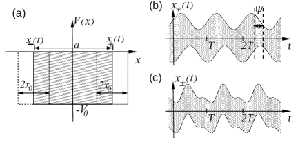
Figure 1: Models for single- and two-parameter driving. Panel a: Laterally driven square potential well as in eq. (1); b: position of the potential well (shaded) as a function of time for two-parameter driving, eq. (2); c: same for single-parameter driving, eqs. (3,4).

We consider a square well with constant depth but lateral driving, i.e., with the positions of its walls depending on time in some arbitrary periodic manner (fig. 1a),

$$V(x,t)=-V_{0}\Big{[}\Theta\big{(}x-x_{-}(t)\big{)}-\Theta\big{(}x-x_{+}(t)\big{)}\Big{]},$$ (1)

where $\Theta(x)$ denotes the Heaviside step function and the wall positions $x_{\pm}(t)$ are periodic functions with the same period $T$. A lateral driving arises naturally from an AC voltage through a Kramers-Henneberger gauge transformation [33, 34]. A phase shift between the walls, equivalent to an oscillating width of the well, can be motivated, e.g., by a finite propagation time across the well of time-dependent perturbations or by a superposed gate voltage. Mass is set $m=1$ throughout.

We assume either two independent harmonic driving forces (“two-parameter driving”) with phase offset $\psi$ (fig. 1b),

$$x_{\pm}(t)=\pm\frac{a}{2}+x_{0}\cos(\omega t\pm\psi/2),\quad\omega=2\pi/T,$$ (2)

where $a$ is the width of the well (in all that follows, $a=2$), or alternatively (“single-parameter driving”) a synchronous motion of both walls (fig. 1c) with the same periodic but otherwise arbitrary time dependence $f(t)$,

$$x_{\pm}(t)=\pm\frac{a}{2}+x_{0}f(t),\quad f(t+T)=f(t).$$ (3)

2.2 Symmetries

In periodically driven scattering, the phase of an incoming trajectory relative to the driving constitutes an additional scattering parameter [19], besides the incoming momentum $p_{\rm in}=\lim_{t\to-\infty}m\dot{x}(t)$. It can be defined, e.g., as $\theta=\omega t_{\rm in}\,{\rm mod}\,2\pi$, with $t_{\rm in}$ the arrival time of the scattered particle, measured by extrapolating its asymptotic incoming trajectory till the origin $x=0$ [29]. As $\theta$ is typically beyond experimental control, directed transport is considered relevant only averaged over $\theta$. In order to avoid a systematic cancellation due to counterpropagating trajectory pairs related by $\mathsf{P}$: ${\bf r}\to-{\bf r}$, ${\bf r}=(p,x)$, $\theta\to-\theta$ (equivalent to $\omega\to-\omega$ or $t\to-t$ for harmonic drivings like (2)), we have to break time-reversal invariance (TRI) of the potential. For eq. (2), this is achieved if $\psi\neq 0$, $\pi$. In eq. (3), it requires a function $f(t)$ without any symmetry or antisymmetry, $f(t_{\pm}-t)\neq\pm f(t)$ for reference times $t_{\pm}$, which excludes in particular harmonic forces. In the sequel, we choose (cf. fig. 1c)

$$f(t)=\cos(\omega t)+\gamma\cos(2\omega t-\phi),\quad\gamma\neq 0,\quad\phi\neq 0\,{\rm mod}\,\pi/2.$$ (4)

For a two-parameter driving, even $\psi$ could be difficult to control. To make sure that currents do not even vanish upon averaging over $\psi$, we prevent the systematic pairing of trajectories related by $\mathsf{P}$ and $\psi\to-\psi$ [29], e.g., by choosing functions for $x_{\pm}(t)$ not connected by any symmetry. For an asymmetric single-parameter driving such as (4), this problem does not arise in the first place.

A relevant issue in the context of symmetry is the energy distribution of incoming and outgoing trajectories. In order to analyze deterministic transport processes based on irregular scattering, it would suffice to consider individual scattering events at a given energy, without assuming specific distributions in the asymptotic regions or reservoirs to keep them constant. The strongly inelastic scattering envisaged here, however, together with symmetry breaking suggest to have a closer look at this aspect.

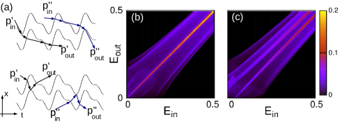
Figure 2: Symmetry and inelastic scattering. Panel a: Systematic pairing of transmitted (above) and reflected (below) trajectories for single-parameter driving with antisymmetric time dependence $f(\pi/2-t)=-f(\pi/2+t)$, eqs. (1,3,4) with $\phi=\pi/2$, see text and fig. 1c. b,c: Probability density distributions $\langle d(E_{\rm in},E_{\rm out})\rangle_{\theta}$ (color code) of outgoing vs. incoming energies for (b) antisymmetric driving as in (a) and (c) asymmetric driving, $\phi=\pi/4$. Other parameter values are $V_{0}=0.75$, $x_{0}=0.1$, $\gamma=0.2$, $\omega=1.0$.

If, for example, we set $\phi=\pi/2\,\hbox{mod}\,\pi$ in eq. (4) (such that $f(\pi/2\omega-t)=-f(\pi/2\omega+t)$), trajectories come in pairs ${\bf r}^{\prime\prime}(t^{\prime\prime})=\mathsf{C}{\bf r}^{\prime}(t^{\prime})$, $\mathsf{C}$: $(p,x,t)\to(p,-x,-t)$ (fig. 2a). As a consequence, incoming and outgoing momenta are interchanged, $p^{\prime\prime}_{\rm in(out)}=p^{\prime}_{\rm out(in)}$, as are the energies $E_{\rm in(out)}$. We illustrate the spread of $E_{\rm out}$ vs. $E_{\rm in}$ in fig. 2b,c in terms of the probability density $\langle d(E_{\rm in},E_{\rm out})\rangle_{\theta}$. In panel (b), the trajectory pairing is reflected in a symmetry of the distribution with respect to the diagonal (the ridge along the diagonal corresponds to elastic processes $E_{\rm in}=E_{\rm out}$). It is absent (c) if the antisymmetry of the driving is broken choosing, e.g., $\phi=\pi/4$ in eq. (4).

Therefore, if $E_{\rm in}$ and $E_{\rm out}$ obey, say, Fermi statistics with the same chemical potential $\mu$ and $E^{\prime}_{\rm in}<\mu<E^{\prime}_{\rm out}$, the process $E^{\prime\prime}_{\rm in}(=E^{\prime}_{\rm out})\to E^{\prime\prime}_{\rm out}(=E^{\prime}_{\rm in})$ is less probable than $E^{\prime}_{\rm in}\to E^{\prime}_{\rm out}$ and a symmetry-induced balance in the reflection probabilities (fig. 2a, lower panel) from either side is broken for inelastic processes, so that they now contribute to the current. More generally, inhomogeneities in the energy distribution, even if they occur identically on both sides, can well enable a finite contribution to transport of processes which otherwise would be suppressed by some symmetry.

We show quantum results for Fermion reservoirs below (fig.8) but mainly consider transport, in classical as well as quantum calculations, as a function of $E_{\rm in}$ without averaging over this quantity.

2.3 Phase-space structures

In the context of Hamiltonian ratchets, the optimal condition to obtain directed currents is not hard chaos but a mixed dynamics with chaotic and regular regions coexisting in an intricately structured phase space [25, 26]. Pumps are no exception to this rule. We therefore focus on systems which pertain only marginally to the regime of chaotic scattering (defined through (i) the existence of a chaotic repeller in phase space, (ii) self-similar deflection functions, and (iii) exponential dwell-time distributions [19]).

Figure 3: Poincaré surfaces of section (PSS, defined by $x=0$, $p>0$). a,b: two-parameter driving, eqs. (1,2), c,d: single-parameter driving, eqs. (1,3,4); a: with TRI, harmonic driving as in eq. (2) with $\psi=0$, inset: periodic orbit underlying the prominent regular island, tracing the position $x(t)$ (short dashed) between $x_{-}(t)$ and $x_{+}(t)$ (full lines); b,c,d: TRI broken with $\psi=\pi/2$ (b), $\gamma=0.1$ (c,d), $\phi=0$ (c), $\pi/2$ (d). Other parameter values as in fig. 2. Large void areas correspond to trajectories not contained in the initial ensemble or intersecting the PSS only a few times.

In fig. 3 we show a set of Poincaré surfaces of section, for two-parameter, eq. (2) (panels a,b) as well as for single-parameter driving, eqs. (3,4) (c,d). In all plots, we observe chaotic regions interspersed with regular islands, characteristic of the KAM scenario [35]. Typically, these islands surround periodic orbits bound in the scattering region and not accessible from outside (see, e.g., the inset in panel a). The phase-space structures clearly reflect the presence or absence of spatiotemporal symmetries of the underlying dynamics, as is evident comparing panels (a) (TR invariant driving) with (b),(c),(d) (TRI broken).

2.4 Directed transport

Moving stepwise from phase-space structures to currents, we analyze the relation between scattering and directed transport on two levels: (i) locally, the outcome of individual scattering processes in terms of asymmetries in reflection and transmission from either side, and (ii) globally, mean currents as functions of scattering parameters like $E_{\rm in}$. They are obtained by averaging discrete outcomes (transmission vs. reflection) over, for example, the phase $\theta$ (see subs. 2.2),

$$\langle I\rangle_{\theta}=\frac{1}{2\pi}\int_{0}^{2\pi}{\rm d}\theta\,([T^{-+}(\theta)+R^{++}(\theta)]-[T^{+-}(\theta)+R^{--}(\theta)]),$$ (5)

where $T^{\pm\mp}$, $R^{\pm\pm}$, denote transmission and reflection probabilities, resp., between the asymptotic regions $x\to\pm\infty$. Their familiar left-right symmetry is generally broken in the absence of a corresponding $\mathsf{P}$-invariance of the Hamiltonian, so that, e.g., reflection from left to left can coexist with transmission from right to left at otherwise identical parameter values.

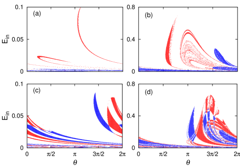
Figure 4: Directed transport in terms of individual scattering processes in parameter space, weak (panels a,c) vs. strong driving (b,d) for two-parameter, eqs. (1,2), (panels a,b) and single-parameter driving, eqs. (1,3,4) (c,d). Parameter values are $V_{0}=0.75$, $x_{0}=0.05$ (a,c), $0.4$ (b,d), $\omega=1.0$, $\psi=\pi/2$ (a,b), $\gamma=0.1$, $\phi=\pi/4$ (c,d). Color code: transmission ${\rm l}\to{\rm r}$ and reflection ${\rm r}\to{\rm r}$ blue, transmission ${\rm r}\to{\rm l}$ and reflection ${\rm l}\to{\rm l}$ red, else white.

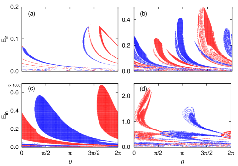
Figure 5: Directed transport in terms of individual scattering processes in parameter space, weak vs. strong symmetry breaking (panels a,b) and slow vs. fast driving (c,d) for single-parameter driving, eqs. (1,3,4). Panel a: weakly broken symmetry, $\gamma=0.01$, b: strongly broken symmetry, $\gamma=1.0$, c: low frequency, $\omega=0.05$, d: high frequency, $\omega=10$. Other parameter values are $x_{0}=0.1$, $\omega=1.0$ (a,b), $\gamma=0.1$ (c,d), $\phi=\pi/2$. Color code as in fig. 4.

We analyze the resulting directed transport “locally in phase space” in figs. 4, 5, contrasting low with high driving amplitude (fig. 4), weak with strong symmetry breaking (5a,b). and slow with fast driving (5c,d). Asymmetric scattering that contributes to directed currents, i.e., exit to the left (right), irrespective of the incoming direction, is labeled red (blue), neutral scattering (same outcome from both sides) white. The emerging structures reflect the relative amount of asymmetric scattering processes in terms of their total area as well as the complexity of the underlying phase space by forming fractals whiich resemble self-similar attraction basins [35].

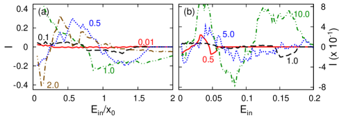
Figure 6: Average currents as functions of various parameters. Single-parameter driving, eqs. (1,3,4). Panel a: current vs. initial energy for different driving amplitudes, $x_{0}=0.01$ (full red line), $0.1$ (dashed, black), $0.5$ (dotted, blue), $1.0$ (dash-double dotted, green), $2.0$ (dash-dotted, brown). Other parameter values are $\gamma=0.1\times x_{0}$, $\phi=\pi/2$, $\omega=1.0$. Panel b: current vs. initial energy for different driving frequencies $\omega=0.5$ (full line, red), $1.0$ (dashed, black), $5.0$ (dotted, blue), $10.0$ (dash-double-dotted, green). Other parameters are $V_{0}=0.75$, $x_{0}=0.1$, $\gamma=0.1$, $\phi=\pi/2$.

Global evidence for directed transport is provided in fig. 6, comparing the dependence of the current on the incoming energy for various values of strength (panel a) and frequency $\omega$ (b) of the driving. As a general tendency, it increases with both parameters but saturates as $\omega$ approaches the inverse time of ballistic flight through the scattering region, confirming our expectation that the mixed character of the dynamics is crucial for current generation. This is also consistent with the fact that currents vanish towards high energy: For $E_{\rm in}\gg V_{0}$, trajectories belong to the regular part of phase space corresponding to quasi-free motion, cf. fig. 3, hence are always transmitted. At lower energies, current sets in as the first trajectories are reflected for only one of the incoming directions and reduces again as the same begins to occur also for the other direction. Superposed on these main trends, we observe frequent sign changes. The corresponding sensitive dependence on the parameters [29, 32] allows for a fine tuning of the current.

As is evident from figs. 4, 5a,b, and 6a, even relatively weak driving or symmetry breaking suffices to achieve considerable transport. Conversely, this indicates that currents due to small unintended asymmetries will be hard to avoid in a real laboratory setup.

3 Quantizing chaotic pumps

3.1 Floquet scattering theory

Scattering at time-dependent potentials is generally inelastic so that standard quantum scattering theory no longer applies. If the driving is periodic, however, large parts of that familiar setting remain intact. A rigorous framework for the treatment of periodically time-dependent quantum systems is provided by Floquet theory [36, 37, 38], worked out for scattering systems in Refs. [39, 40] and applied to quantum pumps in [5]. We here only summarize a few facts directly relevant for us:

• In periodically driven scattering, energy remains conserved ${\rm mod}\,\hbar\omega$, the photon energy associated to the periodic driving. For incoming and outgoing asymptotic energies this means

  $$E_{\rm in/out}(\alpha,n_{\rm in/out})=\epsilon_{\alpha}+n_{\rm in/out}\hbar\omega,$$ (6)

  where $\epsilon_{\alpha}$ is the quasienergy pertaining to a Floquet eigenstate $\alpha$ and $n_{\rm in(out)}$ enumerate incoming (outgoing) discrete Floquet channels. As a consequence, the total energy difference $E_{l}\equiv E_{\rm out}-E_{\rm in}=l\hbar\omega$ is quantized, $l=n_{\rm out}-n_{\rm in}$ counting the total number of photons exchanged with the field.

• The time evolution can be composed as a concatenation of discrete steps of duration $T$ generated by the unitary Floquet operator

  $$\hat{U}_{\rm F}={\cal{T}}\exp\left[-\frac{\rm i}{\hbar}\int_{0}^{T}{\rm d}t\,\hat{H}(t)\right],$$ (7)

  where $\hat{H}(t)$ is the Hamiltonian and $\cal{T}$ effects time ordering. They give rise to a discrete dynamical group and reduce numerical simulations of wavepacket scattering to repeated applications of $\hat{U}_{\rm F}$ [39, 40].

• The “on-quasienergy-shell” scattering matrix $S_{n_{\rm in},n_{\rm out}}(\epsilon)$ [39, 40] is also organized in terms of Floquet channels $n_{\rm in}$, $n_{\rm out}$. For one-dimensional scattering systems, it consists of four blocks $S^{\sigma\tau}$, $\sigma,\tau=-(+)$ denoting the left (right) asymptotic region. We define partial transmission and reflection probabilities as

  $$T_{l}^{\sigma,-\sigma}(E_{\rm in}+E_{l})=|S_{n_{\rm in},n_{\rm out}}^{\sigma,-\sigma}(E_{\rm in})|^{2},\;R_{l}^{\sigma,\sigma}(E_{\rm in}+E_{l})=|S_{n_{\rm in},n_{\rm out}}^{\sigma,\sigma}(E_{\rm in})|^{2},$$ (8)

  and the associated total quantities as

  $$T_{\rm tot}^{\sigma,-\sigma}(E_{\rm in})=\sum_{l=-\infty}^{\infty}T_{l}^{\sigma,-\sigma}(E_{\rm in}),\;R_{\rm tot}^{\sigma,\sigma}(E_{\rm in})=\sum_{l=-\infty}^{\infty}R_{l}^{\sigma,\sigma}(E_{\rm in}).$$ (9)

• In terms of eqs. (9), the pumped probability current from left to right for fixed $E$ is obtained in analogy to the classical probability flow (5) as

  $$I(E_{\rm in})=T_{\rm tot}^{-+}(E_{\rm in})+R_{\rm tot}^{++}(E_{\rm in})-T_{\rm tot}^{+-}(E_{\rm in})-R_{\rm tot}^{--}(E_{\rm in}).$$ (10)

  If we assume the left and right leads to connect to reservoirs, the charge current is given as an average weighted by respective energy distributions $f^{\sigma}(E)$ [5],

  $$\langle I\rangle_{E}=\frac{e}{\hbar}\sum_{l=-\infty}^{\infty}\int_{\max(0,-E_{l})}^{\infty}{\rm d}E\,[T_{l}^{-+}(E)f^{-}(E)-T_{l}^{+-}(E)f^{+}(E+E_{l})].$$ (11)

  For Fermi distributed electrons at zero temperature and identical chemical potentials $\mu=E_{\rm F}$, this means

  $$\langle I\rangle_{E}=\frac{e}{\hbar}\sum_{l=-\infty}^{\infty}\int_{\max(0,-E_{l})}^{\min(E_{\rm F},E_{\rm F}-E_{l})}{\rm d}E\,[T_{l}^{-+}(E)-T_{l}^{+-}(E+E_{l})].$$ (12)

3.2 Numerical methods

The matrix elements $S_{n_{\rm in},n_{\rm out}}^{\sigma,\tau}(\epsilon)$ as basic input to further evaluation of currents (10,11,12) etc. are determined numerically by wavepacket scattering: An initially free wavepacket $|\psi^{\sigma}_{\rm in}\rangle$ at a well-defined wavenumber $k_{0}(\epsilon)=\sqrt{2m\epsilon}/\hbar$ is propagated stroboscopically through the scattering region by repeated application of $\hat{U}_{\rm F}$. Once a suitable termination criterion is met (e.g. when the occupation probability within the interaction region, cf. the integral on the r.h.s. of eq.(15), has decayed to below some threshold value), the final wavepackets $|\psi^{\sigma}_{\rm out}\rangle$ are decomposed into Floquet channels at $k_{l}(E_{\rm in})=\sqrt{2m(E_{\rm in}+E_{l})}/\hbar$, cf. eq. (6), to determine the scattering matrix elements $S_{0,l}^{\sigma,\tau}=k_{0}(E_{\rm in})\psi^{\tau}_{\rm out}\big{(}k_{l}(E_{\rm in})\big{)}/k_{l}(E_{\rm in})\psi^{\sigma}_{\rm in}\big{(}k_{0}(E_{\rm in})\big{)}$. The Floquet operator is efficiently calculated by the $(t,t^{\prime})$-method [41].

Spurious interferences between the reflected and the transmitted wavepacket can occur if periodic boundary conditions are imposed at the ends of the finite spatial box underlying the propagation procedure. To prevent them, we employ absorbing boundaries instead. Specifically, the so-called Smooth Exterior Scaling Complex Absorbing Potentials (SES-CAPs [42]), while cumbersome to handle numerically, keep complications due to the corresponding non-Hermitian terms in the Hamiltonian at a minimum, as they are energy independent and leave the physical potential unscaled.

3.3 Quantum transport

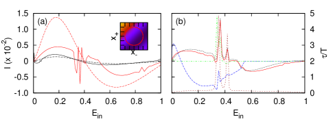
Figure 7: Quantum current as a function of the initial energy. Panel a: Floquet approach, eq. (10) (full lines), compared with adiabatic theory, eqs. (13,14) (dashed), for slow (black, $\omega=0.1$) vs. fast (red, $\omega=1.0$) two-parameter driving, eqs. (1,2). Inset: parameter cycle in $(x_{-},x_{+})$-space (bold red line) and fictitious magnetic field $B(x_{-},x_{+})$, eq. (14) at $E=0.45$, underlying the adiabatic approximation (color code: from black, $B<0$, through red, $B=0$, through yellow, $B>0$). Panel b: Total current for single-parameter driving, eqs. (1,3,4), with $\omega=1.0$, $\phi=\pi/2$ (full line, red), Floquet currents in the elastic and first and second inelastic channels, $n=0,1,2$ (dotted black, dot-dashed green, and dashed blue lines, resp., the latter two amplified by factors $10$ and $5\times 10^{2}$, resp.), and dwell time, eq. (15) (short-dashed brown, rightmost ordinate). Other parameters are $V_{0}=0.75$, $x_{0}=0.1$, $\hbar=0.5$.

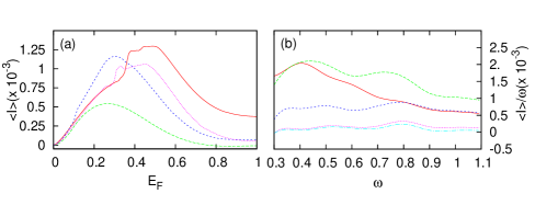
Figure 8: Fermi-averaged quantum current (12) for single-parameter driving, eqs. (1,3,4). Panel a: Mean current vs. Fermi energy $E_{\rm F}$ for frequencies $\omega=0.1$ (full line, red), 0.3 (dashed green), 0.6 (dashed blue), 1.0 (dotted pink). Panel b: Scaled mean current $I/\omega$ vs. frequency $\omega$ at Fermi levels $E_{\rm F}=0.2$ (full line, red), 0.4 (dashed green), 0.6 (dashed blue), 0.8 (dotted pink), 1.0 (dash-dotted bright blue). Other parameters are$V_{0}=0.75$, $x_{0}=0.1$, $\hbar=0.5$.

In order to make contact with the adiabatic approach to pumping and to demonstrate the strongly nonadiabatic character of chaotic pumps, we compare in fig. 7a numerical results for the two-parameter model (2) in the Floquet approach (full lines) with the predictions of the adiabatic scattering approach based on the Berry phase [3] (broken): For a system with a single degree of freedom, two contacts (left, right), and two independently driven parameters $\xi_{1}(t)$, $\xi_{2}(t)$, the probability current through the device is

$$I_{\rm tot}(E)=\frac{-{\rm i}\omega}{4\pi^{2}}\int_{A}{\rm d}^{2}\xi\,B(\boldsymbol{\xi},E).$$ (13)

The area $A$ in parameter space enclosed by the path $\boldsymbol{\xi}(t)=(\xi_{1}(t),\xi_{2}(t))$ (cf. inset in fig. 6a) is penetrated by the “magnetic field”

$$B(\boldsymbol{\xi},E)\!\!=\!\!\left[\partial_{2}S_{\rm tot}^{\sigma\tau}(E)\partial_{1}S_{\rm tot}^{\sigma\tau\dagger}(E)-\partial_{1}S_{\rm tot}^{\sigma\tau}(E)(E)\partial_{2}S_{\rm tot}^{\sigma\tau\dagger}(E)\right]^{++},$$ (14)

with $S_{\rm tot}^{\sigma\tau}(E)=\sum_{n,n^{\prime}}S_{n,n^{\prime}}^{\sigma\tau}(E)$, and $\partial_{i}=\partial/\partial\xi_{i}$. While for slow driving (black, $\omega=0.1$), we find appreciable agreement, the results deviate drastically for fast driving (red, $\omega=1.0$), indicating that strongly nonlinear transport mechanisms are involved.

Adiabatic theory fails for single-parameter pumps, featured in fig. 7b. We decompose the total current (full line) in Floquet channels (dashed). Although the main contribution comes from the elastic channel ($n=0$), inelastic scattering ($n=1,2$) is also present. Sharp resonances in the partial and total currents coincide largely with peaks in the dwell time (dotted brown), measured as the fraction of the wavepacket inside the interaction region summed over stroboscopic time [28],

$$\tau=T\sum_{j=-\infty}^{\infty}\int_{-a/2-x_{0}}^{a/2+x_{0}}{\rm d}x\,|\psi(x,jT)|^{2}.$$ (15)

Sign changes are observed as well. The current even persists upon Fermi averaging (12) (fig. 8). As in the classical case (fig. 5b), it increases with frequency as with energy but saturates for $\omega\approx 1$ and $E_{\rm F}\approx 1$. Scaling the current as $\langle I\rangle_{E}/\omega$ (fig. 8b) reveals this systematic deviation from the proportionality $I\sim\omega$, expected from linear response, for $\omega\gtrsim 1$.

4 Conclusion

Pumping in the non-adiabatic regime of fast and strong driving where nonlinear classical dynamics becomes relevant, remains largely unexplored. As a first survey into this realm, on the classical as well as on the quantum level, we have studied directed transport induced by irregular scattering. In particular, we have pointed out and provided evidence for the possibility of generating currents by driving just a single parameter, which manifestly goes beyond the adiabatic approximation. Their sensitive parameter dependence reflects the underlying chaotic dynamics and suggests to be harnished for control purposes. The classical nonlinearity induces similar nonadiabatic quantum transport: According to quantum adiabatic transport theory [3], single-parameter current generation is impossible. Hence its occurrence for sufficiently strong and/or fast driving cannot be explained by the mere breaking of TRI alone. Analyzing this quantum-classical relation in the numerically very demanding regime of small effective Planck’s constant where semiclassical methods apply [43] remains as a future task.

Our model has been kept utterly simple, focused on the analysis of chaotic scattering and its impact on directed transport. Several options are conceivable to include more realistic details: Many-particle phenomena like charge blocking, dissipation, decoherence, and finite-temperature energy distributions in the reservoirs are obviously relevant. To be adequately treated, they require sophisticated nonequilibrium methods such as the Keldysh Green function technique [10, 44, 45]. Other tempting perspectives to pursue are incorporating internal degrees of freedom, such as in particular spin [32], as well as pumping against a potential gradient [26] and the rectification of noisy input forces.

References

- [1] D.J. Thouless. Phys. Rev. B, 27:6083, 1983.
- [2] B.L. Altshuler and L.I. Glazman. Science, 283:1864, 1999.
- [3] P. Brouwer. Phys. Rev. B, 58:R10135, 1998.
- [4] J. Avron, A. Elgart, G. Graf, and L. Sadun. Phys. Rev. B, 62:R10618, 2000.
- [5] M. Moskalets and M. Büttiker. Phys. Rev. B, 66:205320, 2002.
- [6] D. Cohen. Phys. Rev. B, 68:155303, 2003.
- [7] T.H. Oosterkamp, L.P. Kouwenhoven, A.E.A. Koolen, N.C. van der Vaart, and C.J.P.M. Harmans. Phys. Rev. Lett., 78:1536, 1997.
- [8] R.H. Blick, D.W. van der Weide, R.J. Haug, and K. Eberl. Phys. Rev. Lett., 81:689, 1998.
- [9] E. Prada, P. San-Jose, and H. Schomerus. Phys. Rev. B, 80:245414, 2009.
- [10] Y. Gu, Y. H. Yang, J. Wang, and K. S. Chan. J. Phys.: Cond. Mat., 21:405301, 2009.
- [11] L. E. F. Foa Torres. Phys. Rev. B, 72:245339, 2005.
- [12] M. M. Mahmoodian, L. S. Braginsky, and M. V. Entin. Phys. Rev. B, 74:125317, 2006.
- [13] A. Agarwal and D. Sen. Phys. Rev. B, 76:235316, 2007.
- [14] M. Moskalets and M. Büttiker. Phys. Rev. B, 78:035301, 2008.
- [15] N. Rohling and F. Großmann. Phys. Rev. B, 83:205310, 2011.
- [16] D. Cohen, T. Kottos, and H. Schanz. Phys. Rev. E, 71:035202(R), 2005.
- [17] I. Sela and D. Cohen. J. Phys. A: Math. Gen., 39:3575, 2006.
- [18] S. Hoffmann, M. Hofmann, M. Kira, and S.W. Koch. Semicond. Sci. Technol., 20:S205, 2005.
- [19] U. Smilansky. In M.-J. Giannoni, A. Voros, and J. Zinn-Justin, editors, Chaos and Quantum Physics, volume LII of Les Houches Lectures, page 371. North-Holland–Elsevier, Amsterdam, 1992.
- [20] L. Benet, D. Trautmann, and T.H. Seligman. Cel. Mech. Dyn. Astron., 66:203, 1997.
- [21] D.W. Noid, S.K. Gray, and S.A. Rice. J. Chem. Phys., 84:2649, 1986.
- [22] P. Brumer and M. Shapiro. Adv. Chem. Phys., 70:365, 1988.
- [23] P. Gaspard and S.A. Rice. J. Chem. Phys., 90:2225; ibid. 2242; ibid. 2255, 1989.
- [24] P. Reimann. Phys. Rep., 361:57, 2002.
- [25] H. Schanz, M.-F. Otto, R. Ketzmerick, and T. Dittrich. Phys. Rev. Lett., 87:070601, 2001.
- [26] H. Schanz, T. Dittrich, and R. Ketzmerick. Phys. Rev. E, 71:026228, 2005.
- [27] M. Henseler, T. Dittrich, and K. Richter. Europhys. Lett., 49:289, 2000.
- [28] M. Henseler, T. Dittrich, and K. Richter. Phys. Rev. E, 64:046218, 2001.
- [29] T. Dittrich, M. Gutiérrez, and G. Sinuco. Physica A, 327:145, 2003.
- [30] P. San-Jose, E. Prada, S. Kohler, and H. Schomerus. Phys. Rev. B, 84:155408, 2011.
- [31] S. Flach, O. Yevtushenko, and Y. Zolotaryuk. Phys. Rev. Lett., 84:2358, 2000.
- [32] T. Dittrich and F. Dubeibe. J. Phys. A: Math. Theor., 41:265102, 2008.
- [33] H.A. Kramers. Collected Scientific Papers. North-Holland, Amsterdam, 1956.
- [34] W.C. Henneberger. Phys. Rev. Lett., 21:838, 1958.
- [35] E. Ott. Chaos in dynamical systems. Cambridge University Press, Cambridge (UK), 1993.
- [36] H. Sambe. Phys. Rev. A, 7:2203, 1973.
- [37] J.S. Howland. Indiana Univ. Math. J., 28:471, 1979.
- [38] K. Yajima. J. Math. Soc. Jpn., 29:729, 1979.
- [39] P. Šeba. Phys. Rev. E, 47:3870, 1993.
- [40] P. Šeba and P. Gerwinski. Phys. Rev. E, 50:3615, 1994.
- [41] U. Peskin and N. Moiseyev. J. Chem. Phys., 99:4590, 1993.
- [42] O. Shemer, D. Brisker, and N. Moiseyev. Phys. Rev. A, 71:032716, 2005.
- [43] K. Richter and M. Sieber. Phys. Rev. Lett., 89:206801, 2002.
- [44] B. Wang, J. Wang, and H. Guo. Phys. Rev. B, 65:073306, 2002.
- [45] L. Arrachea and M. Moskalets. Phys. Rev. B, 74:245322, 2006.