Improved Smoothed Analysis of Multiobjective Optimization††thanks: The paper appeared in a preliminary version in the proceedings of STOC 2012 and will appear in JACM.
University of Bonn, Germany
{brunsch,roeglin}@cs.uni-bonn.de )
Abstract
We present several new results about smoothed analysis of multiobjective optimization problems. Motivated by the discrepancy between worst-case analysis and practical experience, this line of research has gained a lot of attention in the last decade. We consider problems in which linear and one arbitrary objective function are to be optimized over a set of feasible solutions. We improve the previously best known bound for the smoothed number of Pareto-optimal solutions to , where denotes the perturbation parameter. Additionally, we show that for any constant the moment of the smoothed number of Pareto-optimal solutions is bounded by . This improves the previously best known bounds significantly.
Furthermore, we address the criticism that the perturbations in smoothed analysis destroy the zero-structure of problems by showing that the smoothed number of Pareto-optimal solutions remains polynomially bounded even for zero-preserving perturbations. This broadens the class of problems captured by smoothed analysis and it has consequences for non-linear objective functions. One corollary of our result is that the smoothed number of Pareto-optimal solutions is polynomially bounded for polynomial objective functions. Our results also extend to integer optimization problems.
1 Introduction
In most real-life decision-making problems there is more than one objective to be optimized. For example, when booking a train ticket, one wishes to minimize the travel time, the fare, and the number of train changes. As different objectives are often conflicting, usually no solution is simultaneously optimal in all criteria and one has to make a trade-off between different objectives. The most common way to filter out unreasonable trade-offs and to reduce the number of solutions the decision maker has to choose from is to determine the set of Pareto-optimal solutions, where a solution is called Pareto-optimal if no other solution is simultaneously better in all criteria.
Multiobjective optimization problems have been studied extensively in operations research and theoretical computer science (see, e.g., [10] for a comprehensive survey). In particular, many algorithms for generating the set of Pareto-optimal solutions for various optimization problems such as the (bounded) knapsack problem [17, 13], the multiobjective shortest path problem [8, 12, 20], and the multiobjective network flow problem [9, 16] have been proposed. Enumerating the set of Pareto-optimal solutions is not only used as a preprocessing step to eliminate unreasonable trade-offs, but often it is also used as an intermediate step in algorithms for solving optimization problems. For example, the Nemhauser–Ullmann algorithm [17] treats the single-criterion knapsack problem as a bicriteria optimization problem in which a solution with small weight and large profit is sought, and it generates the set of Pareto-optimal solutions, ignoring the given capacity of the knapsack. After this set has been generated, the algorithm returns the solution with the highest profit among all Pareto-optimal solutions with weight not exceeding the knapsack capacity. This solution is optimal for the given instance of the knapsack problem.
Generating the set of Pareto-optimal solutions (a.k.a. the Pareto set) only makes sense if few solutions are Pareto-optimal. Otherwise, it is too costly and it does not provide enough guidance to the decision maker. While, in many applications, it has been observed that the Pareto set is indeed usually small (see, e.g., [15] for an experimental study of the multiobjective shortest path problem), one can, for almost every problem with more than one objective function, find instances with an exponential number of Pareto-optimal solutions (see, e.g., [10]).
Motivated by the discrepancy between worst-case analysis and practical observations, smoothed analysis of multiobjective optimization problems has gained a lot of attention in the last decade. Smoothed analysis is a framework for judging the performance of algorithms that has been proposed in 2001 by Spielman and Teng [21] in order to explain why the simplex algorithm is efficient in practice even though it has an exponential worst-case running time. In this framework, inputs are generated in two steps: first, an adversary chooses an arbitrary instance, and then this instance is slightly perturbed at random. The smoothed performance of an algorithm is defined to be the worst expected performance the adversary can achieve. This model can be viewed as a less pessimistic worst-case analysis, in which the randomness rules out pathological worst-case instances that are rarely observed in practice but dominate the worst-case analysis. If the smoothed running time of an algorithm is low and inputs are subject to a small amount of random noise then it is unlikely to encounter an instance on which the algorithm performs poorly. In practice, random noise can stem from measurement errors, numerical imprecision or rounding errors. It can also model arbitrary influences, which we cannot quantify exactly, but for which there is also no reason to believe that they are adversarial.
After its invention in 2001, smoothed analysis has been successfully applied in a variety of contexts, e.g., to explain the practical success of local search methods, heuristics for the knapsack problem, online algorithms, and clustering. A recent survey by Spielman and Teng [22] summarizes some of these results. One of the areas in which smoothed analysis has been applied extensively is multiobjective optimization. In 2003 Beier and Vöcking [3] initiated this line of research by showing that the smoothed number of Pareto-optimal solutions is polynomially bounded for all linear binary optimization problems with two objective functions. This was the first rigorous explanation why heuristics for generating the set of Pareto-optimal solutions are successful in practice despite their bad worst-case behavior. In the last years, Beier and Vöcking’s original result has been improved and extended significantly in a series of papers. A discussion of this work follows in the next section after the formal description of the model.
1.1 Model and Previous Work
We consider a very general model of multiobjective optimization problems. An instance of such a problem consists of objective functions that are to be optimized over a set of feasible solutions for some integer . While the set and the last objective function can be arbitrary, the first objective functions have to be linear of the form for and . We assume without loss of generality that all objectives are to be minimized and we call a solution Pareto-optimal if there is no solution which is at least as good as in all of the objectives and even better than in at least one. We will introduce this notion formally in Section 2. The set of Pareto-optimal solutions is called the Pareto set. We are interested in the size of this set. As a convention, we count distinct Pareto-optimal solutions that coincide in all objective values only once. Since we compare solutions based on their objective values, there is no need to consider more than one solution with exactly the same values.
If one is allowed to choose the set , the objective function , and the coefficients of the linear objective functions arbitrarily, then even for , one can construct instances with an exponential number of Pareto-optimal solutions. For this reason Beier and Vöcking introduced the model of -smooth instances [3], in which an adversary can choose the set and the objective function arbitrarily while he can only specify a probability density function for each coefficient according to which it is chosen independently of the other coefficients. This model is more general than Spielman and Teng’s original two-step model in which the adversary first chooses coefficients which are afterwards subject to Gaussian perturbations. In -smooth instances the adversary can additionally determine the type of noise. He could, for example, specify for each coefficient an interval of length from which it is chosen uniformly at random. The parameter can be seen as a measure for the power of the adversary: the larger the more precisely he can specify the coefficients of the linear objective functions. The aforementioned example of uniform distributions in intervals of length shows that for smoothed analysis becomes a worst-case analysis.
The smoothed number of Pareto-optimal solutions depends on the number of integer variables, the maximum integer , and the perturbation parameter . It is defined to be the largest expected number of Pareto-optimal solutions the adversary can achieve by any choice of , , and the densities . In the following we assume that the adversary has made arbitrary fixed choices for these entities. Then we can associate with every matrix the number of Pareto-optimal solutions in when the coefficients of the linear objective functions take the values given in . Assuming that the adversary has made worst-case choices for , , and the densities , the smoothed number of Pareto-optimal solutions is the expected value , where the coefficients in are chosen according to the densities . For , we call the -th moment of the smoothed number of Pareto-optimal solutions. Here we assume that the adversary has made worst-case choices for , , and the densities that maximize (in general, these are different from the choices that maximize ).
Beier and Vöcking [3] showed that for the binary bicriteria case (i.e., ) the smoothed number of Pareto-optimal solutions is and . The upper bound was later simplified and improved by Beier et al. [2] to . In his PhD thesis [1], Beier conjectured that the smoothed number of Pareto-optimal solutions is polynomially bounded in and for and every constant . This conjecture was proven by Röglin and Teng [18], who showed that for binary solutions and for any fixed , the smoothed number of Pareto-optimal solutions is , where the function is roughly . They also proved that for any constant the -th moment of the smoothed number of Pareto-optimal solutions is bounded by . Moitra and O’Donnell [14] improved the bound for the smoothed number of Pareto-optimal solutions significantly to . However, it remained unclear how to improve the bound for the moments by their methods. Recently a lower bound of for the smoothed number of Pareto-optimal solutions was proven [6].
1.2 Our Results
In this article, we present several new results about smoothed analysis of multiobjective binary and integer optimization problems. Besides general -smooth instances, we additionally consider the special case of quasiconcave density functions. This means that we assume that every coefficient is chosen independently according to its own density function with the additional requirement that for every density there is a value such that is non-decreasing in the interval and non-increasing in the interval . We do not think that this is a severe restriction because all natural perturbation models, like Gaussian or uniform perturbations, use quasiconcave density functions. Furthermore, quasiconcave densities capture the essence of a perturbation: each coefficient has an unperturbed value and the probability that the perturbed coefficient takes a value becomes smaller with increasing distance . We will call these instances quasiconcave -smooth instances in the following.
Beier and Vöcking originally only considered -smooth instances for binary bicriteria optimization problems (i.e., for the case ). The above described canonical generalization of this model to binary multiobjective optimization problems, on which Röglin and Teng’s [18] and Moitra and O’Donnell’s results [14] are based, appears to be very general and flexible at the first glance. However, one aspect limits its applicability severely and makes it impossible to formulate certain multiobjective linear optimization problems in this model. The weak point of the model is that it assumes that every binary variable appears in every linear objective function as it is not possible to set some coefficients deterministically to .
Already Spielman and Teng [21] and Beier and Vöcking [4] observed that the zeros often encode an essential part of the combinatorial structure of a problem and they suggested to analyze zero-preserving perturbations in which it is possible to either choose a density according to which the coefficient is chosen or to set it deterministically to . Zero-preserving perturbations have been studied in [19] and [4] for analyzing smoothed condition numbers of matrices and the smoothed complexity of binary optimization problems. For the smoothed number of Pareto-optimal solutions no upper bounds are known that are valid for zero-preserving perturbations (except trivial worst-case bounds), and in particular the bounds proven in [18] and [14] do not seem to generalize easily to zero-preserving perturbations. In this article, we develop new techniques for analyzing the smoothed number of Pareto-optimal solutions that can also be used for analyzing zero-preserving perturbations.
Theorem 1.
For any , the smoothed number of Pareto-optimal solutions is for quasiconcave -smooth instances with zero-preserving perturbations and for general -smooth instances with zero-preserving perturbations.
Let us remark that the bounds stated in Theorem 1 hold for any and not only for sufficiently large values of . This is why the factor is outside of the -notation. The -notation only refers to the parameters and . For constant like in the binary case the factor is a constant for fixed . In Section 1.3 we will present some applications of zero-preserving perturbations. We will see that they allow us not only to extend the smoothed analysis to linear multiobjective optimization problems that are not captured by the previous model without zero-preserving perturbations, but that they also enable us to bound the smoothed number of Pareto-optimal solutions in problems with non-linear objective functions. In particular, the number of Pareto-optimal solutions for multivariate polynomial objective functions can be bounded by Theorem 1. We say that a -smooth instance has polynomial objective functions if every objective function , , is the weighted sum of monomials, where the adversary can specify a -bounded density on for every weight according to which it is chosen. Denote the total number of monomials by and let denote the maximum degree of the monomials. Then the following corollary holds.
Corollary 2.
For any , the smoothed number of Pareto-optimal solutions is for quasiconcave -smooth instances with polynomial objective functions. For general -smooth instances with polynomial objective functions the smoothed number of Pareto-optimal solutions is .
In addition to zero-preserving perturbations we also study the standard model of -smooth instances. We present significantly improved bounds for the smoothed number of Pareto-optimal solutions and the moments, answering two questions posed by Moitra and O’Donnell [14].
Theorem 3.
For any , the smoothed number of Pareto-optimal solutions is for quasiconcave -smooth instances and for general -smooth instances.
The bound of Theorem 3 for quasiconcave -smooth instances improves the previously best known bound of in the binary case (which is, however, valid also for non-quasiconcave densities) and it answers a question posed by Moitra and O’Donnell whether it is possible to improve the factor of in their bound [14]. Together with the recent lower bound of [6], which is also valid for quasiconcave density functions, this shows that the exponents of both and are linear in .
Theorem 4.
For any and any constant , the -th moment of the smoothed number of Pareto-optimal solutions is for quasiconcave -smooth instances and for general -smooth instances.
This answers a question in [14] whether it is possible to improve the bounds for the moments in [18] and it yields better concentration bounds for the smoothed number of Pareto-optimal solutions. Our results also have immediate consequences for the expected running times of various algorithms because most heuristics for generating the Pareto set of some problem (including the ones mentioned at the beginning of the introduction) have a running time that depends linearly or quadratically on the size of the Pareto set.
The straightforward extension of the Nemhauser-Ullmann algorithm [17] to the multiobjective knapsack problem has, for example, a running time of on instances with items where denotes the Pareto set of the instance that consists only of the first items. (For the running time can be made linear in if the sets are stored in sorted order.) Other examples are the extensions of the Bellman-Ford algorithm and the Floyd-Warshall algorithm to multiobjective shortest path problems (see, e.g., [11]) whose running times depend linearly (for ) or quadratically (for ) on the number of Pareto-optimal solutions in certain subproblems. The improved bounds on the smoothed number of Pareto-optimal solutions and the second moment of this number yield improved bounds on the smoothed running times of these and various other algorithms.
Note that our analysis also covers the general case when the set is an arbitrary subset of . In this case, consider the shifted set for and the functions , defined as for and . The Pareto set with respect to and and the Pareto set with respect to and are identical except for a shift of in the image space. Hence, the sizes of both sets are equal. All aforementioned results can be applied for and , so they also hold for and if one replaces by .
1.3 Applications of Zero-preserving Perturbations
Let us first of all remark that we can assume that the adversarial objective is injective. If not, then let be the values taken by and let . Now, consider an arbitrary injective function and define the new adversarial objective as . Obviously, this function is injective and it preserves the order of the solutions in . This means that if for , then also . Let be a Pareto optimum with respect to and and let , , be all the other solutions for which for all . These are all Pareto optima but, due to our convention, we only count them once. Without loss of generality let be the solution that minimizes among these solutions. Then is also Pareto-optimal with respect to and .
Before we give some applications of zero-preserving perturbations let us remark that in the bicriteria case, which was studied in [3], zero-preserving perturbations are not more powerful than other perturbations because they can be simulated by the right choice of and the objective function .
Assume, for example, that the adversary has chosen and and has decided that the first coefficient of the first objective function should be deterministically set to . Also assume without loss of generality that is injective. We can partition the set into classes of solutions that agree in all components except for the first one. This means that two solutions and belong to the same class if for all . All solutions in the same class have the same value in the first objective as they differ only in the binary variable , whose coefficient has been set to . We construct a new set of solutions that contains for every class only the solution with smallest value in . One can verify that the number of Pareto-optimal solutions is the same with respect to and with respect to because all solutions in are dominated by solutions in . Then we transform the set into a set by dropping the first component of every solution. Furthermore, we define a function that assigns to every solution the same value that assigns to the corresponding solution in . One can verify that the Pareto set with respect to and is identical with the Pareto set with respect to and . The only difference is that in the latter problem we have eliminated the coefficient that is deterministically set to . Such an easy reduction of zero-preserving perturbations to other perturbations does not seem to be possible for anymore.
Path Trading
Berger et al. [5] study a model for routing in networks. In their model there is a graph whose vertex set is partitioned into mutually disjoint sets . We can think of as the Internet graph whose vertices are owned and controlled by different autonomous systems (ASs). We denote by the set of edges inside . The graph is undirected, and each edge has a length . The traffic is modeled by a set of requests, where each request is characterized by its source node and its target node . The Border Gateway Protocol (BGP) determines for each request the order in which it has to be routed through the ASs. We say that a path from to is valid if it connects to and visits the ASs in the order specified by the BGP protocol. This means that the first AS has to choose a path inside from to some node in that is connected to some node . Then the second AS has to choose a path inside from to some node in that is connected to some node and so on. For simplicity, the costs of routing a packet between two ASs are assumed to be , whereas AS incurs costs of for routing the packet inside along path . In the common hot-potato routing, every AS is only interested in minimizing its own costs for each request. To model this, there are objective functions that map each valid path to a cost vector , where

In [5] the problem of path trading is considered. If there is only one request, then no AS has an incentive to deviate from the hot-potato strategy. The problem becomes more interesting if there are multiple requests that have to be satisfied. Consider, for example, the three ASs depicted in Figure 1 and assume that there are three requests , , and . Moreover, assume that the BGP specifies that all requests from to shall be routed directly from AS to AS . If all ASs follow the hot-potato strategy, then they decide for the routes , , and . Each AS incurs costs of for the request and costs of for the request for which .
Now assume that AS routes request from to . Then it incurs costs of (instead of ) for this route, which is worse than if it had chosen the hot-potato route. However, if all ASs agree on this new strategy, then each AS only incurs costs of (instead of ) for the request for which . Hence, the total costs of each AS for satisfying the three requests is instead of .
The path trading problem asks whether there exist routes for given requests such that the total costs of each involved AS is less than or equal to the total costs it would incur if all would follow the hot-potato strategy. Such routes are called feasible path trades.
Consider requests and --paths that comply with the BGP. For an edge let be the number of paths that contain . We can encode the routes by an integer vector consisting of the values . Let denote the set of encodings of all valid routes . The question whether there is a feasible path trade for the requests reduces to the question whether the vector that encodes the hot-potato routes is not Pareto-optimal with respect to and , where the objectives ,
describe the total costs of AS for the routes encoded by . As the Pareto set can be exponentially large in the worst case, Berger et al. [5] proposed to study -smooth instances in which an adversary chooses the graph and a density for every edge length according to which it is chosen. It seems as if we could easily apply the results in [18] and [14] to bound the smoothed number of Pareto-optimal paths because all objective functions are linear in the binary variables , . However, note that different objective functions contain different variables because the coefficients of all with are set to in . This is an important combinatorial property of the path trading problem that has to be obeyed. In the model in [18] and [14] it is not possible to set coefficients deterministically to . In their model, an AS would, with a probability of , incur positive costs for all edges and not only for its own edges that are used, which does not resemble the structure of the problem. Theorem 1, which allows zero-preserving perturbations, yields immediately the following result.
Corollary 5.
The smoothed number of Pareto-optimal valid paths is polynomially bounded in , , and for any constant .
Non-linear Objective Functions
Even though we assumed above that the objective functions are linear, we can also extend the smoothed analysis to non-linear objective functions. We consider first the bicriteria case . As above, we assume that the adversary has chosen an arbitrary set of feasible solutions and an arbitrary injective objective function . In addition to that the adversary can choose arbitrary functions , . The objective function is defined to be a weighted sum of the functions :
where each weight is randomly chosen according to a density given by the adversary. There is a wide variety of functions that can be expressed in this way. We can, for example, express every polynomial if we let be its monomials. Note that the value then depends on the set and the maximum degree of the monomials.
We can linearize the problem by introducing a binary variable for every function . Using the function , defined by , the set of feasible solutions becomes . For this set of feasible solutions we define and as follows:
The problem defined by , , and and the problem defined by , , and are equivalent and have the same number of Pareto-optimal solutions. The latter problem is linear and hence we can apply the result by Beier et al. [2], which yields that the smoothed number of Pareto-optimal solutions is bounded by . This shows in particular that the smoothed number of Pareto-optimal solutions is polynomially bounded in the number of monomials, the maximum integer in the monomials’ ranges, and the density parameter for every polynomial objective function .
We can easily extend these considerations to multiobjective problems with . For these problems the adversary chooses an arbitrary set , numbers , and an arbitrary injective objective function . In addition to that he chooses arbitrary functions for and . Every objective function is a weighted sum
of the functions , where each weight is randomly chosen according to a density chosen by the adversary. Similar to the bicriteria case, also this problem can be linearized. However, the previous results about the smoothed number of Pareto-optimal solutions can only be applied if every objective function is composed of exactly the same functions . Theorem 1 implies that the smoothed number of Pareto-optimal solutions is polynomially bounded in , , and , for any choice of the .
Outline
After introducing some notation in the next section, we present an outline of our approach and our methods in Section 3. In our analysis we will frequently draw upon fundamental properties of Pareto-optimal solutions. These are stated and proven in Section 4. In Section 5 we prove Theorems 3 and 4. In Section 6 we consider zero-preserving perturbations and prove Theorem 1. We conclude the article with some open questions.
2 Notation
For the sake of simplicity we write instead of , even for the adversarial objective . With we refer to the vector . In our analysis, we will shift the solutions by a certain vector and consider the values . For the linear objectives we mean the value , where is well-defined even for a shift vector . For the adversarial objective, however, we define . It should not be confused with for . Note that for Pareto-optimality only the ordering of the solutions with respect to and not the values themselves are of interest. By the definition of , the ordering of the vectors , , equals the ordering of the vectors when considering .
In the whole article let be an arbitrary real for which is integral. Our analyses are valid for all such choices of , but to obtain our results we will consider the limit . Thus, think of as a very small real. Let be a vector such that is an integral multiple of for all . We will call the set an -box and the corner of . For a vector the expression denotes the unique -box for which . We call the -box of and say that lies in . With we denote the set of all -boxes having corners for which . Hence, . If all coefficients of are from , which is true for all models considered in this article, and if for all there is an index such that , which holds with probability in all of our models, then the -box of any vector belongs to . Note that all vectors constructed in this article are from . Hence, without any further explanation we will assume that .
In this article we extensively use tuples instead of sets. The reason for this is that we are not only interested in certain components of a vector or matrix, but we also want to describe in which order they are considered. This will be clear after the introduction of the following notation. Let be positive integers and let , be arbitrary and not necessarily pairwise distinct reals. We define , , and . By and we denote the tuples we obtain by removing all occurrences of elements from that do/do not belong to . We write if and if can be obtained from by removing elements.
Let be a vector and let be a matrix. By we denote the column vector , by we denote the matrix consisting of the rows of matrix (in this order).
For an index set and a vector let denote the set of all solutions such that for all indices . For the sake of simplicity we also use the notation to describe the set for a vector when the components of are labeled by where .
With we refer to the -identity matrix and with to the -matrix whose entries are all . If the number of rows and columns are clear, then we drop the indices.
For a set and a vector we define , the Minkowski sum of and .
Definition 6.
Let be a set of solutions and let be functions.
-
1.
Let be vectors. We say that dominates (with respect to ), if for all and for at least one . We say that dominates strongly (with respect to ), if for all .
-
2.
Let be a vector. We call Pareto-optimal or a Pareto-optimum (with respect to and ), if is an element of and if no solution dominates . We call weakly Pareto-optimal or a weak Pareto-optimum (with respect to and ), if is an element of and if no solution dominates strongly.
We focus on Pareto-optimal solutions. The notions of strong dominance and weak Pareto-optimality are merely used for zero-preserving perturbations.
3 Outline of our Approach
To prove our results we adapt and improve methods from the previous analyses by Moitra and O’Donnell [14] and by Röglin and Teng [18] and combine them in a novel way. Since all coefficients of the linear objective functions lie in the interval , for every solution the vector lies in the hypercube . The first step is to partition this hypercube into -boxes. If is very small (exponentially small in ), then it is unlikely that there are two different solutions and that lie in the same -box unless and differ only in positions that are not perturbed in any of the objective functions, in which case we consider them as the same solution. In the remainder of this section we assume that no two solutions lie in the same -box. Then, in order to bound the number of Pareto-optimal solutions, it suffices to count the number of non-empty -boxes.
In order to prove Theorem 3 we show that for each fixed -box the probability that it contains a Pareto-optimal solution is bounded by for the constant that is hidden in the -notation. This implies the theorem as the number of -boxes is and the exponent of is . Fix an arbitrary -box . In the following we will call a solution a candidate if there is a realization of such that is Pareto-optimal and lies in . If there was only a single candidate , then we could bound the probability that there is a Pareto-optimal solution in by the probability that this particular solution lies in . This probability can easily be bounded from above by in the non-zero-preserving case. However, in principle, every solution can be a candidate and a union bound over all of them leads to a factor of in the bound, which we have to avoid.
Following ideas of Moitra and O’Donnell, we divide the draw of the random matrix into two steps. In the first step some information about is revealed that suffices to limit the set of candidates to a single solution . The exact position of this solution is determined in the second step. If the information that is revealed in these two steps is chosen carefully, then there is enough randomness left in the second step to bound the probability that lies in the -box . In Moitra and O’Donnell’s analysis the coefficients in the matrix are partitioned into two groups. In the first step the first group of coefficients is drawn, which suffices to determine the unique candidate , and in the second step the remaining coefficients are drawn, which suffices to bound the probability that lies in . The second part consists essentially of coefficients, which causes the factor of in their bound.
We improve the analysis by a different choice of how to break the draw of into two parts. As in the previous analysis, most coefficients are drawn in the first step. Only coefficients of are drawn in the second step. However, these coefficients are not left completely random as in [14] because after the other coefficients have been drawn there can still be multiple candidates for Pareto-optimal solutions in . Instead, the randomness is reduced further by drawing linear combinations of these random variables in the first step. These linear combinations have the property that, after they have been drawn, there is a unique candidate whose position can be described by linear combinations that are linearly independent of the linear combinations already drawn in the first step. In [18] it was observed that linearly independent linear combinations of independent random variables behave in some respect similar to independent random variables. With this insight one can argue that in the second step there is still enough randomness to bound the probability that lies in . While the analysis in [18] yields only a bound proportional to , we prove an improved result for quasiconcave densities that yields the desired bound proportional to (see Theorem 40).
In order to bound the moment, we sum the probability that all -boxes simultaneously contain a Pareto-optimal solution over all -tuples of -boxes. We bound this probability from above by for the constant that is hidden in the -notation. Since there are different -tuples of -boxes and the exponent of is , this implies the bound of for the smoothed moment of the number of Pareto-optimal solutions.
Let us fix a -tuple of -boxes. The approach to bound the probability that all of these -boxes contain simultaneously a Pareto-optimal solution is similar to the approach for the first moment. We divide the draw of into two steps. In the first step enough information is revealed to identify for each of the -boxes a unique candidate for a Pareto-optimal solution in . If we do this carefully, then there is enough randomness left in the second step to bound the probability that for every . Again most coefficients are drawn in the first step and some linear combinations of the other coefficients are also drawn in the first step. However, we cannot simply repeat the construction for the first moment independently times because then there might be dependencies between the events for different . In order to bound the probability that in the second step all lie in their corresponding -boxes , we need to ensure that the events are (almost) independent after the information from the first step has been revealed.
The general approach to handle zero-preserving perturbations is closely related to the approach for bounding the first moment for non-zero-preserving perturbations. However, additional complications have to be handled. The main problem is that we cannot easily guarantee anymore that the linear combinations in the second step are linearly independent of the linear combinations revealed in the first step. Essentially, the revealed linear combinations describe the positions of some solutions, which we will call auxiliary solutions in the following. For non-zero-preserving perturbations revealing this information is not critical as no solution has in any objective function exactly the same value as . For zero-preserving solutions it can, however, happen that the auxiliary solutions take exactly the same value as in one of the objective functions. Then there is not enough randomness left in the second step anymore to bound the probability that lies in this objective in the -interval described by the -box .
In the remainder of this section we will present some more details on our analysis. We first present a simplified argument to bound the smoothed number of Pareto-optimal solutions. Afterwards we will briefly discuss which changes to this argument are necessary to bound higher moments and to analyze zero-preserving perturbations.
Smoothed Number of Pareto-optimal Solutions
As an important building block in the proof of Theorem 3 we use an insight from [14] about how to test whether a given -box contains a Pareto-optimal solution. Let us fix an -box with corner . The following algorithm takes as parameters the matrix and the -box and it returns a solution .
The actual function that we use in the proof of Theorem 3 is more complex because it has to deal with some technicalities. In particular, the case that some set is empty, in which and would be undefined in the function above, has to be handled. For the purpose of illustration we ignore these technicalities here and assume that is never empty. The crucial observation that has been made by Moitra and O’Donnell is that if there is a Pareto-optimal solution that lies in , then (assuming that no two solutions lie in the same -box). Hence, the solution returned by the function is the only candidate for a Pareto-optimal solution in . Our goal is to execute the function and to obtain the solution without revealing the entire matrix . We will see that it is indeed possible to divide the draw of into two steps such that in the first step enough information is revealed to execute the function and such that in the second step there is still enough randomness left to bound the probability that lies in .
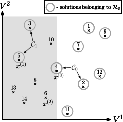
We want to illustrate the case , in which there are one adversarial and two linear objective functions (even though the following reasoning is true for all ). For this, assume that contains a single solution which is Pareto-optimal and that is very close to the corner of which can be assumed if is very small. Then is equivalent to for each .
Consider the situation depicted in Figure 2a. The first and the second objective value of each solution determine a point in the Euclidean plane. The additional value depicted next to this point represents the third objective value of each solution. Let us consider the situation before entering the loop. All points in Figure 2a are encircled meaning that contains all solutions, i.e., . Now let us analyze the loop. The set contains all solutions that have smaller first and second objective values than (gray area in Figure 2b). Among these solutions we pick the one with the smallest third objective value and denote it by . Set contains all solutions with a smaller third objective value (encircled points in Figure 2c). Note that in particular no solution of the gray region is considered anymore. On the other hand, belongs to due to Pareto-optimality.
The set contains all solutions from that have a smaller first objective value than (encircled points in the gray area in Figure 2d). Among these solutions is the one with the smallest second objective value. Set contains all solutions from with a smaller second objective value (encircled points in Figure 2e). This set still contains , but no points from the gray region.
In the final iteration we obtain since there is no restriction in the construction of anymore and since . Solution is among the remaining solutions the one with the smallest first objective value (Figure 2f). This solution equals and is now returned.


Let us now discuss how the draw of can be divided into two steps such that in the first step enough information is revealed to execute the function and such that in the second step there is still enough randomness left to bound the probability that lies in . For this let be a set of indices and assume that we know in advance which values the solutions take at these indices, i.e., assume that we know before executing the function. Then we can reconstruct without having to reveal the entire matrix . This can be done by the following algorithm, which gets as additional parameters the set and the matrix .
The additional restriction of the set does not change the outcome of the function as all solutions generated by the first function are contained in the set defined in line 1 of the second function. Similarly one can argue that the additional restrictions in lines 3 and 5 do not change the outcome of the algorithm because all solutions generated by the first function satisfy the restrictions that are made in the second function. Hence, if , then both functions generate the same .
We will now discuss how much information about needs to be revealed in order to execute the second function, assuming that the additional parameters and are given. We assume that the coefficients are revealed for every and . For the remaining coefficients only certain linear combinations need to be known in order to be able to execute the function. By carefully looking at the function, one can deduce that for only the following linear combinations need to be known:
These terms can be viewed as linear combinations of the random variables , , , with coefficients from . In addition to the already fixed random variables , , , the following linear combinations determine the position of :
An important observation on which our analysis is based is that if the vectors are linearly independent, then also all of the above mentioned linear combinations are linearly independent. In particular, the linear combinations that determine the position of cannot be expressed by the other linear combinations. Usually, however, it is not possible to find a tuple of indices such that the vectors are linearly independent. By certain technical modifications of the function we will ensure that there always exists such a tuple with and that the last index of is determined by the other indices. Since we do not know the tuple and the matrix in advance, we apply a union bound over all valid choices for these parameters, which yields a factor of in the bound for the probability that there exists a Pareto-optimal solution in .
Röglin and Teng [18] observed that the linear independence of the linear combinations implies that even if the linear combinations needed to execute the function are revealed in the first step, there is still enough randomness in the second step to prove an upper bound on the probability that lies in a fixed -box that is proportional to . The bound proven in [18] is, however, not strong enough to improve Moitra and O’Donnell’s result [14] because the dependence on is in the order of which is worse than the dependence of proven by Moitra and O’Donnell. We show that for quasiconcave density functions the dependence in [18] can be improved significantly to , which yields the improved bound of in Theorem 3 for the binary case.
Higher Moments
The analysis of higher moments is based on running the function multiple times. Let us fix a -tuple of -boxes. As described above, we bound the probability that all of them contain a Pareto-optimal solution. For this, we run the function times. In this way, we get for every a sequence of solutions such that is the unique candidate for a Pareto-optimal solution in .
As above, we would like to execute the calls of the function without having to reveal the entire matrix . Again if we know for a subset the values that the solutions , , , take at these positions, then we do not need to reveal the coefficients with to be able to execute the calls of the function. As in the case of the first moment, it suffices to reveal some linear combinations of these coefficients.
In order to guarantee that these linear combinations are linearly independent of the linear combinations that determine the positions of the solutions , , we need to coordinate the calls of the function. Otherwise it might happen that, for example, the linear combinations revealed for executing the first call of the witness function determine already the position of , the candidate for a Pareto-optimal solution in . Assume that the first call of the function returns a sequence of solutions and that is a set of indices that satisfies the desired property that are linearly independent. In order to achieve that all solutions generated in the following calls of the function are linearly independent of these linear combinations, we do not start a second independent call of the function, but we restrict the set of feasible solutions first. Instead of choosing among all solutions from , we restrict the set of feasible solutions for the second call of the function to . Although we do not know in advance, we can assume to know some of its entries due to a technical trick. Essentially, all solutions generated in call of the function have to coincide with in all positions that have been selected in one of the previous calls.
This and some additional tricks allow us to ensure that in the end there is a set with such that all vectors , , are linearly independent. Then we can again use the bound proven in [18] to bound the probability that simultaneously for every from above by a term proportional to . With our improved bound for quasiconcave density functions, we obtain a bound proportional to . Together with a union bound over all valid choices for and the values , , , we obtain a bound of on the probability that all candidates lie in their corresponding -boxes for the constant that is hidden in the -notation. Together with the bound of for the number of -tuples this implies Theorem 4 as the exponent of is .
Zero-preserving Perturbations
If we use the same function as above also for zero-preserving perturbations, then it can happen that there is a Pareto-optimal solution in the -box that does not coincide with the solution returned by the function. This problem occurs, for example, if , which we cannot exclude if we allow zero-preserving perturbations. We recommend to visualize this case for . On the other hand if we knew in advance that , then we could bound the probability of already after the solution has been generated. Hence, if we were only interested in bounding this probability, we could terminate the function already after has been generated. Instead of terminating the function at this point entirely, we keep in mind that has already been determined and we restart the function with the remaining objective functions only.
Let us make this a bit more precise. As long as the solutions generated by the function differ in all objective functions from , we execute the function without any modification. Only if a solution is generated that agrees with in some objective functions, we deviate from the original function. Let denote the objective functions in which coincides with . At this point we can bound the probability that simultaneously for all . In order to also deal with the other objectives , we restart the function. In this restart, we ignore all objective functions in and we execute the function as if only objectives were present. Additionally we restrict in the restart the set of feasible solutions to those that coincide in the objectives with , i.e., to . With similar techniques as in the analysis of higher moments we ensure that different restarts lead to linearly independent linear combinations.
This exploits that every Pareto-optimal solution is also Pareto-optimal with respect to only the objective functions with if the set is restricted to solutions that agree with in all objective functions with . This property guarantees that whenever the function is restarted, is still a Pareto-optimal solution with respect to the restricted solution set and the remaining objective functions.
It can happen that we have to restart the function times before a unique candidate for a Pareto-optimal solution in is identified. As in each of these restarts at most solutions are generated, the total number of solutions that is generated can increase from , as in the case of non-zero-preserving perturbations, to roughly . The set of indices restricted to which these solutions are linearly independent has a cardinality of at most . The reason for this increase is that we have to choose more indices to obtain linear independence due to the fixed zeros. Taking a union bound over all valid choices of , of the values that the generated solutions take at these positions, and of the possibilities when and due to which objectives the restarts occur, yields Theorem 1. This theorem relies again on the result about linearly independent linear combinations of independent random variables from [18] and its improved version for quasiconcave densities that we show in this article.
4 Properties of (Weak) Pareto-optimal Solutions
In this section we will identify the main properties of (weakly) Pareto-optimal solutions that lay the foundation for all variants of the function. In the model without zero-preserving perturbations we only need properties of Pareto optima. In the model with zero-preserving perturbations, however, much more work has to be done and there we need the notion of weak Pareto optimality.
We start with an observation that is valid for both Pareto-optimal solutions and weak Pareto-optimal solutions.
Proposition 7.
Let be a set of solutions, let be functions, let be a (weak) Pareto optimum with respect to and , and let be a subset of solutions that contains . Then is (weakly) Pareto-optimal with respect to and .
The core idea of the functions is given by the following lemma and Corollary 9. It implies that if is Pareto-optimal with respect to and , then is also Pareto-optimal with respect to and (cf. function described in Section 3). Given this as the induction step, it yields that is Pareto-optimal with respect to and . This means that in iteration we obtain because .
Lemma 8.
Let be a set of solutions, let , , be functions, and let be a weak Pareto optimum with respect to and . We consider the set of solutions that dominate strongly with respect to .
-
(I)
If , then is weakly Pareto-optimal with respect to and .
-
(II)
If , then let . Then . Furthermore, if , then is weakly Pareto-optimal with respect to and .
Proof.
Claim (I) holds due to the definition of weak Pareto optimality. Let us consider Claim (II). If the inequality does not hold, then dominates strongly with respect to . This is a contradiction since is weakly Pareto-optimal with respect to and .
Now let us show that is weakly Pareto-optimal with respect to and if . The condition ensures that . Assume to the contrary that there exists a that dominates strongly with respect to . Since , this implies . Due to we obtain the contradiction , where the second inequality follows from the definition of and . ∎
If the functions in Lemma 8 are injective, we can also obtain a statement about Pareto optima.
Corollary 9.
Let be a set of solutions, let , , be functions, where are injective, and let be a Pareto optimum with respect to and . We consider the set of solutions that dominate strongly with respect to .
-
(I)
If , then is Pareto-optimal with respect to and .
-
(II)
If , then let . Then . Furthermore, is Pareto-optimal with respect to and .
Proof.
First of all we observe that a solution dominates with respect to if and only if dominates strongly with respect to . This is due to the injectivity of the functions . Consequently, Claim (I) follows from the definition of Pareto optimality. Let us consider Claim (II). Assume to the contrary that . In this case, the solution would dominate with respect to contradicting the assumption that is Pareto-optimal. Hence, .
Due to Lemma 8, is weakly Pareto-optimal with respect to and because every Pareto optimum is also a weak Pareto optimum. As these functions are injective, is even Pareto-optimal with respect to and . ∎
For the model with zero-preserving perturbations we need one more lemma that allows us to handle non-injectivity appropriately.
Lemma 10.
Let be a set of solutions, let , , be functions, and let be a Pareto optimum with respect to and . Furthermore, let be a tuple of indices and let be a subset of . Then is Pareto-optimal with respect to and .
Proof.
Assume to the contrary that is not Pareto-optimal. Then there exists a solution such that dominates with respect to . Since for all , solution also dominates with respect to . This contradicts the assumption that is Pareto-optimal. ∎
5 Non-zero-preserving Perturbations
5.1 Smoothed Number of Pareto-optimal Solutions
To prove Theorem 3 we assume without loss of generality that and consider the function given as Algorithm 1 which we call the function. It is very similar to the one suggested by Moitra and O’Donnell, but with an additional parameter . This parameter is a tuple of forbidden indices: it restricts the set of indices we are allowed to choose from. For the analysis of the smoothed number of Pareto-optimal solutions we will set . The parameter becomes important in the next section when we analyze higher moments.
Let us give some remarks about the function. Note that since is no restriction if . In Line 1 ties are broken by taking the lexicographically first solution . For the index in Line 1 exists because which implies .
Unless stated otherwise, we assume that the following OK-event occurs. This event occurs if for every and for arbitrary two distinct solutions and if for all there is an index for which . Amongst others, the first property ensures that there is a unique in Line 1 and that the functions are injective. The latter property, which holds with probability , ensures that for all vectors . Later we will see that the OK-event occurs with sufficiently high probability.
Before we start to analyze the function, let us discuss the differences between the function described in Section 3 and the function given as Algorithm 1. As described in Section 3 for the illustrative case , the parameters and play exactly the same role if assuming that the OK-event holds. As stated earlier, the additional parameter in the function has no meaning for the analysis of the first moment. To prove Theorem 3, we simply set it to the empty tuple. The case (Line 1) is the interesting case, which is also captured by the function . The case (Line 1) is the technical case. Here it is only important that we choose an index that is not an element of and that the vector is defined such that coincides with in all components and that it does not coincide with in component . Note that the vector as we define it in Line 1 is not necessarily a solution from .
In the remainder of this section we only consider the case that is Pareto-optimal, that is an arbitrary index tuple with pairwise distinct indices, and that the number of indices contained in is at most . This ensures that the indices exist.
Lemma 11.
The call returns the vector .
Proof.
We show the following claim by induction on .
Claim 1.
For all , solution is Pareto-optimal with respect to and .
Proof of Claim 1.
Note that the functions are injective due to the assumption that the OK-event occurs. This allows us to apply Corollary 9. Recalling that for every index tuple , Claim 1 is true for by assumption and due to Proposition 7.
Now let us assume that the claim holds for some value and consider set . We distinguish between two cases. If , then and the claim follows from the induction hypothesis, from Corollary 9 (I), and from Proposition 7. If , then for . Hence, the claim follows from the induction hypothesis, from Corollary 9 (II), and from Proposition 7. ∎
In accordance with Claim 1, we obtain for that is Pareto-optimal with respect to and . In particular, , i.e., . This solution will be returned in iteration . ∎∎
At a first glance it seems odd to compute a solution by calling a function with as parameter. However, we will see that not all information about is required to execute the call . To be a bit more precise, the indices and the entries at the positions of the vectors constructed during the execution of the function suffice to simulate the execution of without knowing completely (see Lemma 14). We will call these information a certificate (see Definition 12). For technical reasons we will assume that we also know the entries of the vectors at position and, for the analyis of higher moments, also at further positions.
For our purpose it is not necessary to know how to obtain the required information about to reconstruct it. It suffices to know that the set of possible certificates is sufficiently small (see Lemma 17) and that for at least one of them the simulation of the execution of returns (see Lemma 14). This is one crucial property which will help us to bound the expected number of Pareto-optimal solutions.
Definition 12.
Let be the vectors and be the index tuple constructed during the call and set and . We call the pair for the -certificate of . The pair for is called the restricted -certificate of . We call a pair a (restricted) -certificate, if there exist a realization such that the OK-event occurs and a Pareto-optimal solution such that is the (restricted) -certificate of . By we denote the set of all restricted -certificates.
The notation used in this section is summarized in Table 1.
| set of feasible solutions | |
|---|---|
| linear objective functions | |
| adversarial objective function | |
| coefficients of for | |
| probability density of for and | |
| matrix of coefficients of | |
| number of Pareto-optimal solutions for | |
| event that for every and for arbitrary two distinct solutions and that for all there is an index for which | |
| set of all -boxes having corners for which | |
| -box for which | |
| vectors constructed during the call of Algorithm 1 | |
| sets constructed during the call of Algorithm 1 | |
| sets constructed during the call of Algorithm 1 | |
| index tuple constructed during the call of Algorithm 1 | |
| -certificate of where | |
| restricted -certificate of where | |
| (restricted) -certificate, i.e., there exist a realization such that the OK-event occurs and a Pareto-optimal solution such that is the (restricted) -certificate of | |
| set of all restricted -certificates | |
| shift vector used in Algorithm 2 |
For the analysis of the first moment we only need restricted -certificates. Our analysis of higher moments requires more knowledge about the vectors than just the values for . The additional indices are, however, depending on further calls of the function which we do not know a priori. This is why we have to define two types of certificates. For the sake of reusability we formulate some statements more general than necessary for this section.
Lemma 13.
Let be an arbitrary realization for which the OK-event occurs, let be a Pareto-optimal solution with respect to and , and let be the restricted -certificate of . Then consists of pairwise distinct indices and
where each ‘’ can be an arbitrary value from (different ‘’-entries can represent different values) and where for a value can be an arbitrary value from .
Proof.
Lemma 11 implies that the last column of equals . Hence, we just have to consider the first columns of . Note that and . The construction of the sets yields (see Lines 1, 1, and 1). Index is always chosen such that : If it is constructed in Line 1, then . Since in this case we have
index cannot be an element of . In Line 1, index is explicitely constructed such that . The same argument holds for index . Hence, the indices of are pairwise distinct.
Now, consider the column of corresponding to vector for . If , then the form of the column follows directly from the construction of in Line 1 and from the fact that the indices of are pairwise distinct. If , then
i.e., coincides with in all indices . By the choice of in Line 1 we get . This concludes the proof. ∎
Let be the -certificate of and let be a tuple of pairwise distinct indices. As mentioned before, our goal is to execute the function without revealing the entire matrix . For this we consider the following variant of the function given as Algorithm 2 that uses information about given by the index tuple , the matrix with columns , a shift vector and the -box instead of vector itself. The meaning of the shift vector will become clear when we analyze the probability of certain events. We will see that not all information about needs to be revealed to execute the new function, i.e., we have some randomness left which we can use later. With the choice of the shift vector we can control which information has to be revealed for executing the function.
Lemma 14.
Let be the -certificate of , let be an arbitrary tuple of pairwise distinct indices, let , let be an arbitrary vector, and let . Then the call returns vector .
Before we give a formal proof of Lemma 14 we try to give some intuition for it. Instead of considering the whole set of solutions we restrict it to vectors that look like the vectors we want to reconstruct in the next iterations, i.e., we intersect the current set with the set in iteration . In this way we only deal with subsets of the original sets, but we do not lose the vectors we want to reconstruct since . This restriction to the essential candidates of solutions allows us to execute this variant of the function with only partial information about .
Proof.
Let , , and denote the sets and vectors constructed during the execution of the call and let , , and denote the sets and vectors constructed during the execution of call . We prove the following claims simultaneously by induction.
Claim 2.
for all .
Claim 3.
for all for which .
Claim 4.
for all and all for which .
Proof of Claim 2, Claim 3, and Claim 4.
Let us first focus on the shift vector and compare Line 1 of the first function (Algorithm 1) with Line 2 of the second function (Algorithm 2). The main difference is that in the first version we have the restriction , whereas in the second version we seek for solutions such that . As is the corner of the -box , those restrictions are equivalent for solutions since
The first inequality is due to the occurrence of the OK-event.
Now we prove the statements by downward induction over . Let . Lemma 13 yields for all , i.e., because . Consequently, (Claim 2). Consider an arbitrary index for which . Then
For the induction step let . By the observation above we have
Since , we obtain . We first consider the case which implies and in accordance with Lemma 11 since . Then
According to Lemma 13, all vectors coincide with on the indices as . Thus, . As due to Claim 2 of the induction hypothesis, we obtain (Claim 2). For Claim 3 nothing has to be shown here. Let be an index for which . Then by Claim 4 of the induction hypothesis, , and consequently (Claim 4).
Finally, let us consider the case . Claim 4 of the induction hypothesis yields . Since and , also and, thus, . Hence, as (Claim 3). The remaining claims have only to be validated if . Then
because , and
With the same argument used for the case we obtain and, hence, (Claim 2). Consider an arbitrary index for which . Then
In particular, (see Line 1) and, hence, because . Furthermore, due to the induction hypothesis, Claim 4, and . Consequently, (Claim 4). ∎
As mentioned earlier, with the shift vector we control which information of has to be revealed to execute the call . While Lemma 14 holds for every vector , we have to choose carefully for our probabilistic analysis to work. We will see that the choice , given by
| (1) |
is appropriate since for all and (cf. Lemma 19). Recall that is the index that has been added to in the definition of the -certificate to obtain and note that . Moreover, for every index the value is given in the last column of (see Lemma 13). Hence, if is the -certificate of , then vector can be defined when a tuple and the matrix are known; we do not have to know the solution itself.
For bounding the number of Pareto-optimal solutions consider the functions parameterized by an arbitrary restricted -certificate , and an arbitrary -box , defined as follows: if the call returns a solution for which , and otherwise.
Corollary 15.
Assume that the OK-event occurs. Then the number of Pareto-optimal solutions is at most
Proof.
Let be a Pareto-optimal solution, let be the restricted -certificate of , and let . Due to Lemma 14, returns vector . Hence, . It remains to show that the assignment given in the previous lines is injective. Otherwise we would count the occurence of two distinct Pareto-optimal solutions and only once in the sum stated in Corollary 15.
Let and be distinct Pareto-optimal solutions and let and be the restricted -certificates of and , respectively. If , then and are mapped to distinct triplets. Otherwise, and, hence, because of the OK-event and . Consequently, also in this case and are mapped to distinct triplets. ∎
Corollary 15 immediately implies a bound on the expected number of Pareto-optimal solutions.
Corollary 16.
The expected number of Pareto-optimal solutions is bounded by
where denotes the event that the call returns a vector such that .
Proof.
By applying Corollary 15, we obtain
We will see that the first term of the sum in Corollary 16 can be bounded independently of and that the limit of the second term tends to for . First of all, we analyze the size of the restricted certificate space.
Lemma 17.
The size of the restricted certificate space for is bounded by
Proof.
Exactly indices are created during the execution of the call if the OK-event occurs and if is Pareto-optimal with respect to . The index is determined deterministically depending on the indices . Matrix of every restricted -certificate is a -matrix with entries from . Hence, the number of possible restricted -certificates is bounded by . ∎
Let us now fix an arbitrary -certificate , a tuple , and an -box . We want to analyze the probability where . By and we denote the part of the matrix that belongs to the indices and to the indices , respectively. We apply the principle of deferred decisions and assume that is fixed as well, i.e., we will only exploit the randomness of .
As motivated above, the call can be executed without the full knowledge of . To formalize this, we introduce matrices that describe the linear combinations of that suffice to be known:
| (2) |
for where are the columns of matrix and . Note that the matrices depend on the pair and on the vector .
Lemma 18.
Let be an arbitrary shift vector and let and be two realizations of such that and for all indices and all columns of the matrix . Then the calls and return the same result.
Lemma 18 states that for different realizations and of the modified function outputs the same result. Actually, in the proof we will even see that the complete execution of both calls is identical. This means that solution is already determined if these realizations are known. However, there is still randomness left in the objective values which allows us to bound the probability that falls into box (see Corollary 21).
Proof.
We fix an index and analyze which information of is required for the execution of the call . For the execution of Line 2 we need to know for solutions in all iterations . Since we assume to be known, this means that
must be revealed. For vector is a column of . The execution of Line 2 does not require further information about : The only iteration where we might need information about is iteration . However, as , we obtain
because all solutions agree on the entries with indices . Since is known, can be determined without any further information. Note that this does not imply that is already specified.
It remains to consider Line 2. Only in iteration we need information about . In that iteration it suffices to know for every solution . Hence, for , , the linear combinations
must be revealed. For , vector is a column of .
As and agree on all necessary information, both calls return the same result. ∎
We will now see why defined in Equation (1) is a good shift vector.
Lemma 19.
Let where . Then
where denotes the matrix for which . Each ‘’-entry can be an arbitrary value from and each ‘’-entry can be an arbitrary value from . Different ‘’-entries as well as different ‘’-entries can represent different values.
Proof.
Lemma 20.
For all the columns of the matrix and the vector are linearly independent.
Proof.
Let for all . It suffices to show that the columns of the submatrix and the vector are linearly independent. Consider the matrix . Due to Lemma 19 the last rows of form a lower triangular matrix and the entries on the principal diagonal are from the set . Consequently, the vectors are linearly independent. As these vectors are the same as the columns of matrix plus vector (see Equation 2), the claim holds for . Now let . We consider an arbitrary linear combination of the columns of and the vector and show that it is if and only if all coefficients are .
As the vectors are linearly independent, we first get for , which yields due to and, finally, because of . This concludes the proof. ∎
Corollary 21.
Let . For an arbitrary restricted -certificate the probability of the event is bounded by
and by
if all densities are quasiconcave.
Proof.
Event occurs if the output of the call is a vector for which . We apply the principle of deferred decisions and assume that is fixed arbitrarily. Now let us further assume that the linear combinations of given by the columns of matrix are known for all . This means that for some fixed values we consider all realizations of for which the linear combinations of given by the columns of equal these values. In accordance with Lemma 18, vector is therefore already determined, i.e., it is the same for all realizations of that are still under consideration.
The equality holds if and only if
holds for all , where is the corner of . Since
for the vector , this is equivalent to the event that
where is an interval of length depending on and hence on the linear combinations of given by the matrices . By we denote the -dimensional hypercube with side length defined by the intervals .
For all let be the matrix consisting of the columns of and the vector . These matrices form the diagonal blocks of the matrix
Lemma 20, applied for , implies that matrix has full rank. We permute the columns of to obtain a matrix whose last columns belong to the last column of one of the matrices . This means that the last columns of are . Let the rows of be labeled by assuming that . We introduce random variables , , , labeled in the same fashion as the rows of . Event holds if and only if the linear combinations of the variables given by the last columns of fall into the -dimensional hypercube depending on the linear combinations of the variables given by the remaining columns of . The claim follows by applying Theorem 40 for the matrix and and due to the fact that the number of columns of is . Hence,
in general and
if all densities are quasiconcave. The different bounds for general densities and quasiconcave densities come solely from Theorem 40. ∎
Proof of Theorem 3.
We begin the proof by showing that the OK-event is likely to happen. For all indices and all solutions the probability that is bounded by . To see this, choose one index such that and apply the principle of deferred decisions by fixing all coefficients for . Then the value must fall into an interval of length . The probability for this is bounded from above by . A union bound over all indices and over all pairs for which yields .
Let . We set
With we obtain
The first inequality is due to Corollary 16. The second inequality is due to Corollary 21. The third inequality stems from Lemma 17. Since this bound is true for every for which is integral, it also holds for the limit . Hence, we obtain
Substituting and by their definitions yields
for general densities and
for quasiconcave densities. ∎
5.2 Higher Moments
The basic idea behind our analysis of higher moments is the following: If the OK-event occurs, then we can count the power of the number of Pareto-optimal solutions by counting all -tuples of -boxes where each -box contains a Pareto-optimal solution . We can bound this value as follows: First, call to obtain a vector and consider the index tuple that contains all indices created in this call and one additional index. In the second step, call to obtain a vector and consider the tuple consisting of the indices of , the indices created in this call, and one additional index. Now, call and so on. For the call to be well-defined, in Section 5.1 we assumed . Consequently, here we have to ensure that , i.e., . We can assume this for fixed integers and because all of our results are presented in -notation.
If is a tuple of Pareto-optimal solutions with for , then due to Lemma 11. As in the analysis of the first moment, we use the variant of the function that uses certificates of the vectors instead of the vectors itself to simulate the calls. Hence we can reuse several statements of Section 5.1.
Let us remark that for bounding the moment of the smoothed number of Pareto-optimal solutions we also have to consider -tuples of -boxes for which for some indices . This might seem critical as both boxes contain the same Pareto-optimal solution (if such a solution exists) which could cause problems due to dependencies. We resolve this problem by using different shift vectors and for reconstructing the vectors and with the function.
Unless stated otherwise, let be a realization such that the OK-event occurs and fix arbitrary solutions with for that are Pareto-optimal with respect to .
Definition 22.
Let and let be the -certificate of defined in Definition 12, . We call the pair for , , and , the (restricted) -certificate of . We call a pair a -certificate, if there is a realization such that the OK-event occurs and if there are Pareto-optimal solutions such that is the -certificate of . By we denote the set of all -certificates.
Note that and for .
We now consider the functions , parameterized by an arbitrary -certificate and a vector of -boxes, which is defined as follows: if for all the call returns a solutions such that , and otherwise. Recall that the vector is defined in Equation 1.
Corollary 23.
Assume that the OK-event occurs. Then the power of the number of Pareto-optimal solutions is at most
Proof.
The power of the number of Pareto-optimal solutions equals the number of -tuples of Pareto-optimal solutions. Let be such a -tuple, let be the -certificate of , and let . Due to Lemma 14, returns vector for all . Hence, for . As in the proof of Corollary 15 we have to show that this assignment is injective.
Let and be distinct -tuples of Pareto-optimal solutions, i.e., there is an index such that , and let and be their -certificates. If , then both tuples are mapped to distinct triplets. Otherwise, and, thus, because of the OK-event and . Consequently, also in this case and are mapped to distinct triplets. ∎
Corollary 23 immediately implies a bound on the moment of the number of Pareto-optimal solutions.
Corollary 24.
The moment of the number of Pareto-optimal solutions is bounded by
where denotes the event that .
We omit the proof since it is exactly the same as the one of Corollary 16.
Lemma 25.
The size of the certificate space is bounded by
Proof.
Let be an arbitrary -certificate. Each matrix is a -matrix with entries from . The tuple can be written as
created by successive calls of the function, where the indices are chosen deterministically in Definition 12. Since the claim follows. ∎
Corollary 26.
Let . For an arbitrary -certificate and an arbitrary vector of -boxes the probability of the event is bounded by
and by
if all densities are quasiconcave.
Proof.
For and consider the matrices for defined in Equation (2). Due to Lemma 18 the output of the call is determined if and the linear combinations for all indices and all columns of the matrix are given. With the same argument as in the proof of Corollary 26 event occurs if and only if falls into some -dimensional hypercube with side length depending on the linear combinations . In this notation, is short for .
Now, consider the matrix
Note that . Due to Lemma 19, is a lower block triangular matrix, due to Lemma 20 the columns of are linearly independent. Hence, matrix is an invertible matrix and the same holds for the block diagonal matrix
We permute the columns of to obtain a matrix where the last columns belong to the columns . We assume the rows of to be labeled by where and introduce random variables , , , indexed the same way as the rows of . Event holds if and only if the linear combinations of the variables given by the last columns of fall into the -dimensional hypercube with side length depending on the linear combinations of the variables given by the remaining columns of . The claim follows by applying Theorem 40 for the matrix and and due to the fact that the number of columns of is . ∎
Proof of Theorem 4.
In the proof of Theorem 3 we showed that the probability that the OK-event does not hold is bounded by . Let . We set
Then we obtain
The first inequality is due to Corollary 24. The second inequality is due to Corollary 26. The third inequality stems from Lemma 25. Since this bound is true for every for which is integral, it also holds for the limit . Hence, we obtain
Substituting and by their definitions yields
for general densities and
for quasiconcave densities. ∎
The proof of Theorem 4 yields that for
where
With the following Corollary we bound the probability that exceeds a certain multiple of . We obtain a significantly better concentration bound than the one we would obtain by applying Markov’s inequality for the first moment.
Corollary 27.
The probability that the number of Pareto-optimal solutions is at least for some is bounded by
Proof.
Let be the real for which , i.e.,
Observing that for all and setting yields
The first inequality is Markov’s inequality. The second inequality only holds if . However, for the inequality is trivially true. ∎
6 Zero-preserving Perturbations
Our analysis of Theorem 1 holds for instances with the following property: There exists a partition of such that, for all and for all , the coefficient is not deterministically set to if and only if . This means that exactly of the coefficients are perturbed and that the value only depends on the entries of for which . All other objective functions do not depend on these entries. Furthermore, we require for all .
With the next two lemmas we show that if Theorem 1 holds for instances that have the form described above, then it also holds for all other instances with a slightly larger constant that is hidden in the -notation.
Lemma 28.
Without loss of generality in each objective function except for the adversarial one there are more than perturbed coefficients, i.e., coefficients that are not deterministically set to .
Proof.
For an index let be the tuple of indices for which is a perturbed coefficient, i.e., a coefficient which is not set to deterministically. Let be the tuple of indices for which , let , and consider the decomposition of into subsets of solutions , . Let be an arbitrary solution. If is Pareto-optimal with respect to and , then is also Pareto-optimal with respect to and due to Lemma 10. As all remaining objective functions , , have more than perturbed coefficients, the instance with these objective functions and as set of feasible solutions has the desired form and we can apply Theorem 1 for each of these instances. Since we now have instances, each having linear and one adversarial objective, we can bound the number of Pareto-optimal solutions by
where and denote the exponents of and in the bound stated in Theorem 1. These exponents depend on the number of non-adversarial objectives and whether the densities are quasiconcave or not. Since they are monotonically increasing, which particularly implies and , we can bound the number of Pareto-optima simply by
Hence, it suffices to show that
as the additional factor can be hidden in the -notation. This inequality is equivalent to showing that for and . Note that . By a chain of equivalences we obtain
Applying the inequality yields
This concludes the proof. ∎
Lemma 29.
Without loss of generality for every exactly one of the coefficients is perturbed, whereas the others are deterministically set to .
Let us remark that we can transform every instance that has not the form stated in Lemma 29 into an instance with this form. We will show that this transformation does not increase the size of the Pareto-set for any realization of the coefficients. Hence, the bound from Theorem 1 that applies for the modified instance also applies for the original instance. However, our transformation increases the dimension of the set from to . Hence, we lose a factor of in the bound which we can hide in the -notation since we have to apply this transformation only once.
Proof.
We first show how to decrease the number of indices for which is perturbed to at most one. For this, let
be the set of feasible solutions that contains for every the solution that consists of copies of . For we define a linear objective function in which all coefficients with are deterministically set to . The coefficients are chosen as the coefficients , i.e., either randomly according to a density or deterministically. The objective function maps every solution to . The instance consisting of and the objective functions has the desired property that every variable appears in at most one of the objective functions and it has the same smoothed number of Pareto-optimal solutions as the instance consisting of and the objective functions . For every for which none of the coefficients is perturbed we can eliminate the corresponding variable from .
This shows that every -smooth instance with can be transformed into another -smooth instance with with in which every variable appears in exactly one objective function and that has the same smoothed number of Pareto-optimal solutions. As the bound proven in Theorem 1 depends polynomially on the number of variables, we lose only a constant factor (with respect to , , and ) by going from to . This constant is hidden in the -notation. ∎
In the remainder of this chapter we focus on instances having the structure described in Lemma 28 and Lemma 29. Then is a partition of , where denotes the tuple of indices for which is perturbed.
We consider the variant of the function given as Algorithm 3, referred to as the function, which gets as parameters besides the usual , , and , a set of indices of objective functions and a call number . In a call of the function only the adversarial objective function and the objective functions with are considered. The set of solutions is restricted to solutions that agree with in all positions with . Additionally, as in the function, only solutions are considered that agree with in all positions . By the right choice of , we can avoid choosing an index multiple times in different calls of the function. The parameter simply corresponds to the number of the current call of the function. The function always returns some subset of .
Let us give some remarks about the function. As a convention we set (cf. Line 3). This is only important in the case where , i.e., in the first call.
As in the function, if iteration is reached in a certain call (this does not have to be the case), then we obtain since (see Line 3) is no restriction for . For the definition of in Line 3, ties are broken by taking the lexicographically first solution. Though we did the same in the function, it is much more important here. In the model without zero-preserving perturbations the functions are injective with probability . If this is the case, then no ties have to be broken. In the model with zero-preserving perturbations, the functions can be non-injective with probability : If there are two distinct solutions for which , then .
The index defined in Line 3 is the number of the last call in which the objective function has been considered. The index defined in Line 3 is the number of the iteration in call number of in which the next recursive call of was made. We will see that, if the last call of the function is the call with number , then for each and there is at least one index for which , i.e., the objective function has been considered until the end. Furthermore, the indices are defined for . For the simulation of the function information about the solutions and the indices are required. For the simulation of the function we additionally need the values and to know when to make a new recursive call (in iteration in the call with number ) and which objectives to consider (objective will be considered in the call with number if and only if ).
In Line 3 it is always possible to find an index on which the current vector and disagree because this line is only reached if , i.e., if . In order for Line 3 to be feasible, we have to guarantee that . This follows since we assumed in accordance with Lemma 28 and because there are at most calls of with non-empty with at most iterations each, and in each iteration at most one index from is added to . Note that it would be more precise to introduce the notation rather than (cf. Line 3 and Line 3). Furthermore, we could also write instead of . For the sake of readability we decided to drop these additional indices and refer to index and tuple of iteration of call in our proofs.
Before we analyze the function, let us discuss similarities and differences to the function. The initial calls and are very similar. All objectives are considered. Furthermore, and . Line 3 can be ignored in this call since . Also the loop of the function is very similar to the loop of the function. The sets and and the solution are defined the same way as the sets and and the solution in the function.
However, there are two main differences to the function in the body of the loop that are due to the two additional issues we have to deal with when considering zero-preserving perturbations. First it is possible that for some of the indices . This happens if (otherwise, it happens with probability ) and is a fundamental issue. If we would proceed running the loop as we do it in the function, then we might lose the crucial property that the function returns if is Pareto-optimal. The tuple contains the problematic indices for which . If , then we proceed more or less as we did in the function (see Line 3 and Line 3). As discussed above, the case has to be treated differently. In this case we make use of Lemma 10 which implies that, if is Pareto-optimal, then it is also Pareto-optimal with respect to and (cf. Line 3 of the current call and Line 3 of the next call).
The second difference due to another issue with zero-preserving perturbations can be sketched as follows. In each iteration of the function one index is chosen. Since in the model without zero-preserving perturbations all coefficients are perturbed, we can then exploit the randomness in the coefficients . In the model with zero-preserving perturbations under the assumption given by Lemma 29, for each index exactly one of the coefficients is perturbed while the others are . Hence, we choose one index for each objective to ensure that we have one perturbed coefficient per objective. These indices are chosen only for (see Line 3). This is due to the fact that for our analysis to work we need the additional property that which is impossible for by the definition of and the requirement . However, as from now on we do not consider the objectives for anymore, we do not have to choose indices for .
In the remainder of this section we only consider the case that is Pareto-optimal. Unless stated otherwise, we assume that the following -event occurs. This event occurs if for every and for every two solutions for which . We will later see that the -event occurs with sufficiently high probability.
Lemma 30.
The call returns the set , where .
Lemma 30 was also stated in the conference version ([7], Lemma 25) but Claim 1 of the proof was not correct. Here, we rely on the concept of weak Pareto-optimality (see Definition 6) and its properties (Lemma 8) since we cannot guarantee to be Pareto-optimal in every iteration. However, the Pareto-optimality holds at the beginning of every call to the function.
Proof.
Let us consider an arbitrary call for . First we show the following claim by induction on .
Claim 5.
In every iteration that is reached, is weakly Pareto-optimal with respect to and .
Proof of Claim 5.
To begin with, consider . As is Pareto-optimal with respect to and , is also Pareto-optimal with respect to and
due to Lemma 10. Consequently, is also Pareto-optimal with respect to and due to Proposition 7. Note that this property is even stronger than weak Pareto-optimality. We will need this strong version in the induction step when .
Now consider a iteration that is reached and assume that the induction hypothesis is true for . We consider iteration where is defined, and distinguish between two cases. If , then is weakly Pareto-optimal with respect to and due to the induction hypothesis, Lemma 8 (I), and Proposition 7.
Let us consider the more interesting case . Since iteration is reached, there is no call of the function in iteration , i.e., in iteration . The induction hypothesis and Lemma 8 (II) yield .
We will show that even . For this, we assume to the contrary that and distinguish between the cases and .
-
1.
If , then we obtain and since . Hence, dominates with respect to which contradicts the fact that is Pareto-optimal with respect to and .
-
2.
If , then implies as we assume that the -event occurs. Consequently, in iteration , which contradicts the previous observation that in that iteration.
This concludes the proof of Claim 5. ∎
With Claim 5 we are now able to show that a call terminates without a further call to the function if and only if . Note that one direction is trivial.
Claim 6.
Consider an arbitrary call . If , then this call results in another call to the function (and does not terminate in Line 3).
Proof of Claim 6.
Let us assume that there is no further call to the function until iteration , i.e., we reach iteration . In accordance with Claim 5, is weakly Pareto-optimal with respect to and . Now let us consider iteration . We obtain since there are no restrictions in this iteration. Consequently, because . The solution minimizes among all solutions from . On the other hand, cannot dominate strongly. Hence, , i.e., as we assumed that the -event occurs. Therefore, , i.e., , and thus, the function is called in Line 3. ∎
According to Claim 6 there will be recursive calls until a call of the form . This call immediately returns the set in Line 3. Since , we obtain
Now consider call number and the iteration in this call in which has been called. In this iteration, since Line 3 is reached. Hence, there is at least one index , and for these indices, is set to in Line 3. Now, as the next call is of the form , this implies , i.e., all values for have been set by now and, thus,
i.e., the number of the call we currently consider.
Consider the solution defined in Line 3 and let be the tuple of call . Since this implies . Hence, for all by definition of in Line 3. On the other hand,
The first inclusion is due to the definition of in Line 3. The second inclusion is due to the observation that always due to the construction of the sets in Line 3 and Line 3. The construction of in Line 3 yields the third inclusion. Hence, for all , and according to the previous observations, even for all . Consequently, . Summarizing the previous results, we obtain that the call ends up in the call for some index tuple which immediately returns the set . ∎∎
Like for the simple function, we show that it is enough to know some information about the run of the function to reconstruct the solution . As before, we call this data the certificate of .
Definition 31.
Let and for be the indices and be the vectors constructed during the execution of . Furthermore, consider the tuple at the moment when the last call to the function terminates. The pair for , , and , is called the -certificate of . We label the columns of by . Moreover, we call a pair a certificate if there is some realization such that the -events occurs and if there exists a Pareto-optimal solution such that is the -certificate of . By we denote the set of all certificates.
We assume that the indices and (and hence also the indices ) are implicitly encoded in a given certificate. Later we will take these indices into consideration again when we count the number of possible certificates.
Lemma 32.
Let be a realization for which the -event occurs and let be a -certificate of some Pareto-optimal solution . Let be of the form
For a fixed index let
where . Then is of the form
where each ‘’ can be an arbitrary value from (different ‘’-entries can represent different values) and where for a value can be an arbitrary value from .
Proof.
Consider the call and all subsequent calls . By definition of we have (see Line 3, Line 3, and Line 3). In each call where one vector is constructed in each iteration . Also, in each iteration except for the last iteration of the call, when for the first and the last time, one index is chosen and added to . Since consists of the chosen indices and the additional index , matrix is a square matrix.
We first consider the last column of . As is the last vector constructed before is removed from , index must be an element of in iteration of call , i.e., . Hence, the last column of has the claimed form because .
Now consider the remaining columns of . Due to the construction of the set in Line 3, Line 3, and Line 3, all vectors coincide with in the previously chosen indices . As in the case vector is an element of and in the case vector is constructed appropriately, the upper triangle of , excluding the principal diagonal, has the claimed form. The form of the principal diagonal follows from the choice of index : In Line 3 we chose such that , in Line 3 we construct explicitely such that . ∎
Like in the model without zero-preserving perturbations, our goal is to execute the function without revealing the entire matrix . For this we now consider a variant of the function given as Algorithm 4 which gets as additional parameters the -certificate of , a shift vector , the -box , and a set of solutions that are still under consideration. Recall that at the beginning of every call to the original function the set of solutions that have still to be considered is restricted to a subset of (see Line 3). The huge amount of information that is necessary to restrict the current set of solutions to those that still have to be considered is not given by the -certificate of . Thus, we keep track of this set of remaining solutions by passing it as a parameter. We will see how to update this set without too much knowledge about (cf. Line 4 of Algorithm 4).
It is important to break ties in Line 4 the same way as we did in the original function, i.e., we take the lexicographically first solution.
Lemma 33.
Let be the -certificate of , let be an arbitrary vector, and let . Then the call returns .
Before we give a formal proof of Lemma 33 we try to give some intuition for it. As for the simple variant of the function we restrict the set of solutions to vectors that look like the vectors we want to reconstruct in the next iterations of the current call, i.e., we intersect the current set with the set in iteration . In this way we only deal with subsets of the original sets, but we do not lose the vectors we want to reconstruct. In order to reconstruct the vectors, we need more information than in the simple variant: we need to know in which iterations the recursive calls of are made, in each call we need to know which objective functions must not be considered anymore, and for each of these objective functions we need to know the vector . The information when the recursive calls are made and which objective functions must not be considered anymore is given in the certificate: The variable contains the iteration number when the recursive call is made. The index contains the number of the call where index has to be removed from . Hence, index is removed in the iteration of call . If we can reconstruct and the vector in the iteration where we make the recursive call, then we can also reconstruct the bits of at indices for all indices because for these indices (cf. Line 4).
Proof.
We compare the executions of and and show the following claim by induction on .
Claim 7.
If there is a call of the form during the execution of the call , then there is also a call of the form for during the execution of the call .
Proof of Claim 7.
For the case it is true if we recall the convention that . Now let us consider an arbitrary call and assume that Claim 7 holds for . Hence, we can assume that there are calls of the form and for . We now show that both calls are executed essentially the same way. Formally, we prove the following claims by induction on , where , , , , and refer to the sets, vectors, and tuples from the call .
Claim 8.
for all .
Claim 9.
for all for which .
Claim 10.
for all and all for which .
Proof of Claim 8, Claim 9, and Claim 10.
We apply a downward induction on . For the beginning, consider . We have
Due to the construction of the vectors and the definition of ,
for all (see Lemma 32). The inclusion yields
for all . Consequently, . For Claim 9 nothing has to be shown in the initial step of the induction. Let us consider Claim 10 and let be an arbitrary index for which . Then
Furthermore, for every index tuple due to the definition of . Consequently, .
For the induction step let . Due to the occurence of the -event and the fact that , we obtain
Since , we obtain . First, we consider the case which implies and . The inequality follows from the fact that in iteration the function is called (Line 3 of Algorithm 3) which implies . In this case,
where is the updated index tuple . Due to the construction of the vectors (see Lemma 32) and the definition of the vectors , we know that
for all . As , this implies
As in accordance with the induction hypothesis, Claim 8, we obtain . For Claim 9 nothing has to be shown here. Let be an arbitrary index for which . Then by Claim 10 of the induction hypothesis, , and consequently .
Let us finally consider the case . Claim 10 of the induction hypothesis yields . Since and , also and, thus, . Hence, as . Claim 8 and Claim 10 have only to be validated if , i.e., we can assume that . Then
because , and
With the same argument used for the case we obtain
and, hence, . Consider an arbitrary index for which . Then
In particular, (see Line 3) and, hence, because . Furthermore, due to the induction hypothesis, Claim 10, and . Consequently, . ∎
The induction step of the proof of Claim 7 follows from the three claims above: Let us assume that there is a call of the form . By the definition of , this call is executed in iteration of call . Consequently, . Applying Claim 10 for and , we obtain . As , the inequalities hold, which are equivalent to due to the occurence of the -event. Furthermore, by the definition of . Hence, (see Line 4), i.e., . Moreover, in accordance with Claim 9. In iteration of the call Line 4 is reached. By the definition of the values we obtain , and hence, for all due to the definition of . In Line 4, there is a call of the form . The correctness of Claim 7 follows because
where is the parameter from the call , and because
∎
By the choice of the vector we can control which information about has to be known in order to be able to execute the call . While Lemma 33 is correct for every choice of , we have to choose carefully in order for the following probabilistic analysis to work. Later we will see that , given by
| (3) |
is well-suited for our purpose. Recall that are the indices that have been added to in the definition of the -certificate to obtain . Furthermore, is given by the last column of for every index (cf. Lemma 30). Hence, vector can be defined with the information that is contained in the -certificate of ; we do not have to know the vector itself.
In the next step, we bound the number of Pareto-optimal solutions. For this, consider the following function , parameterized by an arbitrary certificate and an arbitrary -box , that is defined as follows: if returns a set such that , and otherwise.
Corollary 34.
Assume that the -event occurs. Then the number of Pareto-optimal solutions is at most
Proof.
Let be a Pareto-optimal solution, let be the -certificate of , and let . Due to Lemma 33, returns . Hence, . It remains to show that this function defined within the previous lines is injective. Let and be distinct Pareto-optimal solutions and let and be the -certificates of and , respectively. If , then and are mapped to distinct triplets. Otherwise, and, hence, because of the -event. Consequently, also in this case and are mapped to distinct triplets. ∎
Corollary 34 immediately implies a bound on the expected number of Pareto-optimal solutions.
Corollary 35.
The expected number of Pareto-optimal solutions is bounded by
where denotes the event that the call returns a set such that .
Proof.
By applying Corollary 34, we obtain
We will see that the first term of the sum in Corollary 35 can be bounded independently of and that the second term tends to for . First of all, we analyze the size of the certificate space.
Lemma 36.
The size of the certificate space is bounded by
Proof.
Consider the execution of the call and let be the maximum of the values . Including this call with number , there can be at most calls to the function except for the call with number that terminates due to . This is because in each of the other calls at least one index is removed from the tuple . Hence, . Consequently, there are at most possibilities for these numbers. In the call, the iteration number is an element of , and hence, there are at most possibilities to choose iteration numbers . In each iteration, at most indices are added to the tuple . As there are at most calls and at most iterations each call, tuple contains at most indices in total. Hence, there are at most
choices for . Once is fixed, also the indices in are fixed because the indices added to in Definition 31 are determined by . The tuple contains indices. In each call , at most vectors are generated. Hence, matrix has at most columns and at most rows. This yields the claimed bound
In the next step we analyze how much information of is required in order to perform the call for a fixed certificate . We will see that does not need to be revealed completely and that some randomness remains even after the necessary information to perform the call has been revealed. This is the key observation for analyzing the probability . For this, let be an arbitrary realization, i.e., we do not condition on the -event anymore. Let for . We apply the principle of deferred decisions and assume that for every the coefficients of belonging to indices are fixed arbitrarily. We denote this part of by and concentrate on the remaining part of which we denote by .
As in the model with non-zero-preserving perturbations, the call can be executed without the full knowledge of . We write the linear combinations of of the calls and of call that suffice to be known into the following matrices and , respectively:
for , where are the columns of matrix . The index denotes the index for which in the call of the function, i.e., is the objective function in in the call and it is not considered anymore in iterations .
Note that the matrices and depend, among others, on the choice of . Furthermore, the indices are determined by the certificate . To be precise, the indices , which are implicitely given by the certificate , contain the information which objectives are still under consideration in a certain call of the function: These are all objectives for which .
Observe that matrix has
columns and matrix has
columns. The last equation is due to the fact that in each call in each iteration one index is chosen. In call one index is chosen in each iteration . The equation follows since contains one index more than the number of indices that are chosen during the execution of the function (see Definition 31). Moreover, observe that all entries of and are from .
Lemma 37.
Let be an arbitrary shift vector, let be an arbitrary certificate, and let and be two realizations for which and for all indices and all columns of one of the matrices and . Then for every -box the calls and return the same result.
Proof.
We fix an index and analyze which information of is required for the execution of the call . By the construction of index we know that only in the calls information about the function must be available as in all subsequent calls this function is not considered anymore.
Since in call we consider only vectors that coincide with one of the vectors (see Line 4) in the indices , it suffices to know all linear combinations
For all call numbers and all iterations in these calls the vector is a column of matrix .
It remains to analyze which information of is required in the call of the function. First, we observe that . This is due to the fact that , i.e., , since this is the iteration when is removed from tuple . On the other hand, , which means that for all indices , where denote the indices tuple consists of in call . Hence, as .
There are only three lines where information about is required: Line 4, Line 4, and Line 4. For Line 4 the values
from iteration down to iteration are needed. The vectors are columns of matrix . In Line 4 no additional information about is required since all considered vectors agree on indices with each other. For Line 4 only in iteration the values
for are required. Observe that the vectors
for are columns of matrix .
As and agree on all necessary information, both calls return the same result. ∎
In the remainder of this section we assume that and the -box are fixed. In accordance with Lemma 37, the output of the call is determined if the linear combinations of given by the columns of the matrices and are fixed arbitrarily, i.e., it does not depend on the remaining randomness in the coefficients. We are interested in the event , i.e., in the event that the output is a set such that . Since is a -certificate of for some and , the output is always of the form due to Lemma 33. Hence, event occurs if and only if for all indices the relation holds for some interval of length that depends on the linear combinations of given by and for all indices .
Lemma 38.
For every fixed index the columns of matrix , of matrix , and the vector are linearly independent.
Proof.
Consider the square matrix consisting of the vectors , for and . Matrix can be obtained from the matrix of Lemma 32 by subtracting the vector from all of its columns. Due to Lemma 32 and due to the construction of (see Equation 3) matrix is a lower triangular matrix and the elements of the principal diagonal are from the set . This is because for and for all , where for represents an arbitrary value from not equal to . Hence, the vectors are linearly independent.
The columns of and are linear combinations of the vectors , whereas the columns of matrix are the remaining columns of matrix . As the vectors are linearly independent, it suffices to show that the columns of matrix and vector are linearly independent. For this, we consider an arbitrary linear combination of the columns of matrix and vector and show that it is if and only if all coefficients are . For sake of simplicity, we drop the index in the remainder of this proof and write , , and instead of , , and , respectively.
If , then this equation is equivalent to
Therefore, all coefficients are due to the linear independence of the vectors . If , which is the only case remaining due to previous observations, then the equation is equivalent to
The linear independence of the vectors implies for , , and . Consequently, also and, thus, . This means that all coefficients are . In both cases, the linear independence of the columns of and the vector follows. ∎
Corollary 39.
Let . For an arbitrary certificate the probability of the event is bounded by
and by
if all densities are quasiconcave.
Proof.
For a fixed index we write the columns of matrix , of matrix , and vector into one matrix (the number of columns is
due to previous observations) and consider the matrix
This matrix has full rank due to Lemma 38. Now we permute the columns of to obtain a matrix whose last columns belong to the last column of one of the matrices . This means that the last columns are
For all and every index let be the coefficient of . Event holds if and only if the linear combinations of the variables given by the last columns of fall into a -dimensional hypercube depending on the linear combinations of the variables given by the remaining columns. The claim follows by applying Theorem 40 for matrix and due to the fact that (see proof of Lemma 36). ∎
Proof of Theorem 1.
We begin the proof by showing that the -event is likely to happen. For all indices and all solutions for which the probability that is bounded by . To see this, choose one index for which and apply the principle of deferred decisions by fixing all coefficients for arbitrarily. Then the value must fall into an interval of length . The probability for this is bounded by . A union bound over all indices and over all pairs for which yields
Let . We set
Then we obtain
The first inequality is due to Corollary 35. The second inequality is due to Corollary 39. The third inequality stems from Lemma 36. Since this bound holds for any for which is integral, it also holds for the limit . Hence, we obtain
Substituting and by their definitions yields
for general densities and
for quasiconcave densities. ∎
7 Some Probability Theory
In this chapter we lay the probabilistic foundation of this article. We consider linearly independent linear combinations of independent random variables and show that they behave to some extent like independent random variables.
Let be independent random variables with densities for all and let be an integer matrix. Furthermore, let be an -dimensional random vector whose entries are linear combinations of the random variables , and let be an arbitrary function that maps every tuple to a -dimensional hypercube with side length . We want to bound the probability that the random vector falls into the random hypercube from above.
Before we state the main theorem of this section, let us discuss two special cases. One simple case is when the matrix is of the form . In this case, the random variables , , and , , are independent. In order to bound the probability , we can apply the principle of deferred decisions and assume that the outcome of the variables has been revealed by an adversary, say for . Hence, the hypercube is fixed and not random anymore. However, we still have not revealed the outcome of the random variables . As the random variables are independent, we obtain
Observe that we used the simple structure of twice: First, we obtained independence which is why the first equation holds. Second, the event can be directly translated into the event that only depends on the random variables and the hypercube . In general, all random variables and a more complex set that depends on the last rows of have to be considered.
Now let us consider a second special case in which each of the last rows of is a linear combination of the first rows . In particular, for every index we can write as
for appropriate coefficients . As the function we consider the function that maps a tuple to the hypercube , where is defined as
With this choice and the notation we obtain
for all . Hence, falls into the hypercube for every realization of the random variables . Consequently, . The reason why we can define a function with such a property is that the outcome of the random variables is determined when the outcome of the random variables has been revealed since the last rows of can be expressed as linear combinations of the first rows of . Hence, in this special case we cannot obtain any non-trivial bound.
The following theorem claims a non-trivial bound for the probability that the random vector falls into the hypercube for the case when the rows of matrix are linearly independent. The first inequality of Theorem 40 has been shown for binary matrices by Röglin and Teng [18] (see Lemma 3.3). Their proof can be easily generalized to arbitrary integer matrices. For the sake of completeness we state it here.
Theorem 40.
Let be integers and let be independent random variables, each with a probability density function , let be a matrix of rank , let be an integer, let
be the linear combinations of given by , and let be a function mapping a tuple to a hypercube with side length . Then
If all densities are quasiconcave, then even the stronger bound
holds.
Theorem 40 states that, for quasiconcave densities, linearly independent linear combinations of independent random variables almost behave like independent random variables when considering the event with respect to and : The bound in Theorem 40 deviates from the bound derived for the special case for and for (see beginning of this section) only by a factor of .
Proof.
First of all we show that we can assume w.l.o.g. that . Otherwise, we can choose indices for which the matrix is a full-rank square submatrix of . For the sake of simplicity let us assume that for . We apply the principle of deferred decisions and assume that are fixed arbitrarily to some values .
Let , , , and . Let us further introduce the random vector
and the function
Observing that
we obtain
The probability of the last event can be bounded by applying Theorem 40 for the -matrix .
In the remainder of this proof we assume that . As matrix is a full-rank square matrix, its inverse exists and we can write
where denotes the common density of the variables and denotes the common density of the variables . The second equality is due to a change of variables, the first inequality stems from the fact that since is an integer matrix.
In general, we can bound the integral in the formula above by
where the first inequality is due to the fact that all variables can only take values in the interval as all entries of matrix are from and as all variables can only take values in the interval .
To prove the statement about quasiconcave functions we first consider arbitrary rectangular functions, i.e., functions that are constant on a given interval, and otherwise. This will be the main part of our analysis. Afterwards, we analyze sums of rectangular functions and, finally, we show that quasiconcave functions can be approximated by such sums.
Lemma 41.
For let , let be an interval of length , and let be the function
Moreover, let be the function and let be an invertible matrix. Then
where and where the sum runs over all tuples for which .
Proof.
Function takes the value on the -dimensional box and is otherwise. Hence,
for
where is the projection matrix that removes the last entries from a vector of length . In the remainder of this proof we bound the volume of where . Let and be the left and the right bound of interval , respectively. For an index tuple , , and a bit tuple , let
be one of the -dimensional faces of . We show that . Let , i.e., there is a vector such that . Now, consider the polytope
where and for and . This polytope is bounded and non-empty because . Consequently, there exists a basic feasible solution . As there are variables and constraints, this solution has at least zero-entries, i.e., there are indices such that either (in that case set ) or (in that case set ) for all . Now, consider the vector . We obtain and for all . Hence, for and , and thus .
Due to this observation we can bound the volume of by . It remains to show how to bound the volume . For the sake of simplicity we only consider in the following analysis. Let be the function , where and . Using function is the canonical way to describe the affine subspace defined by face : it adds the fixed coordinates of to a given vector of length . Hence, function , restricted to the domain , is bijective. With we obtain
In general, the second equality only holds if is injective. If is not injective, then is not full-dimensional, i.e., , and since is affine linear. Hence, the second equality also holds in the case when is not injective.
Matrix is an -submatrix of . Thus, , and we obtain the bound
In the next step we generalize the statement of Lemma 41 to sums of rectangular functions.
Corollary 42.
Let be positive integers, let be a non-negative real, let be an interval of length , and let be the function
, . Furthermore, let be the function , let be the function , and let be an invertible matrix. Then
where and and where the first sum runs over all tuples for which .
Proof.
For indices let . This function is of the form assumed in Lemma 41 and takes only values and . We can write function as
For the sake of simplicity we write instead of and instead of . We can bound the integral as follows:
where the second inequality is due to Lemma 41. Now,
which completes the proof of Corollary 42. ∎
To finish the proof of Theorem 40 we round the probability densities as follows: For an arbitrarily small positive real let , i.e., we round up to the next integral multiple of . As the densities are quasiconcave, there is a decomposition of such that where
where are intervals of length and are positive reals. The second property is the interesting one and stems from the quasiconcaveness of . Informally speaking the two-dimensional shape bounded by the horizontal axis and the graph of is a stack of rectangles aligned with axes (see Figure 3). Therefore, the sum of the rectangles’ heights which appears in the formula of Corollary 42 is approximately . Without the quasiconcaveness might be unbounded.
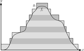
Applying Corollary 42, we obtain
Since and , this implies
As this bound is true for arbitrarily small reals , we obtain the desired bound of
8 Conclusions and Open Problems
With the techniques developed in this article we settled two questions posed by Moitra and O’Donnell [14]: For quasiconcave densities we showed that the exponent of in the bound for the smoothed number of Pareto-optimal solutions is exactly . Moreover, we significantly improved on the previously best known bound for higher moments of the smoothed number of Pareto-optima by Röglin and Teng [18].
Maybe even more interesting are our results for the model of zero-preserving perturbations suggested by Spielman and Teng [21] and Beier and Vöcking [4]. For this model we proved the first non-trivial bound on the smoothed number of Pareto-optimal solutions. We showed that this result can be used to analyze multiobjective optimization problems with polynomial and even more general objective functions. Furthermore, our result implies that the smoothed running time of the algorithm proposed by Berger et al. [5] to compute a path trade in a routing network is polynomially bounded for every constant number of autonomous systems. We believe that there are many more such applications of our result in the area of multiobjective optimization.
There are several interesting open questions. First of all it would be interesting to find asymptotically tight bounds for the smoothed number of Pareto-optimal solutions. There is still a gap between our upper bound of for quasiconcave -smooth instances and the best lower bound of [6]. Only for the case we can show that the upper bound is tight [6].
Especially for zero-preserving perturbations there is still a lot of work to do. We conjecture that our techniques can be extended to also bound higher moments of the smoothed number of Pareto-optima for -smooth instances with zero-preserving perturbations. However, we feel that even our bound for the first moment is too pessimistic as we do not have a lower bound showing that setting coefficients to can lead to larger Pareto sets. It would be very interesting to either prove a lower bound that shows that zero-preserving perturbations can lead to larger Pareto-sets than non-zero-preserving perturbations or to prove a better upper bound for zero-preserving perturbations.
References
- [1] René Beier. Probabilistic Analysis of Discrete Optimization Problems. PhD thesis, Universität des Saarlandes, 2004.
- [2] René Beier, Heiko Röglin, and Berthold Vöcking. The smoothed number of Pareto optimal solutions in bicriteria integer optimization. In Proceedings of the 12th International Conference on Integer Programming and Combinatorial Optimization (IPCO), pages 53–67, 2007.
- [3] René Beier and Berthold Vöcking. Random knapsack in expected polynomial time. Journal of Computer and System Sciences, 69(3):306–329, 2004.
- [4] René Beier and Berthold Vöcking. Typical properties of winners and losers in discrete optimization. SIAM Journal on Computing, 35(4):855–881, 2006.
- [5] André Berger, Heiko Röglin, and Ruben van der Zwaan. Path trading: Fast algorithms, smoothed analysis, and hardness results. In Proceedings of the 10th International Symposium on Experimental Algorithms (SEA), pages 43–53, 2011.
- [6] Tobias Brunsch, Navin Goyal, Luis Rademacher, and Heiko Röglin. Lower bounds for the average and smoothed number of pareto-optima. Theory of Computing, 2014. to appear.
- [7] Tobias Brunsch and Heiko Röglin. Improved smoothed analysis of multiobjective optimization. In Proceedings of the 44th Annual ACM Symposium on Theory of Computing (STOC), pages 407–426, 2012.
- [8] H. William Corley and I. Douglas Moon. Shortest paths in networks with vector weights. Journal of Optimization Theory and Application, 46(1):79–86, 1985.
- [9] Matthias Ehrgott. Integer solutions of multicriteria network flow problems. Investigacao Operacional, 19:229–243, 1999.
- [10] Matthias Ehrgott. Multicriteria Optimization. Springer, 2005.
- [11] Matthias Ehrgott and Xavier Gandibleux. Multiobjective combinatorial optimization. In Matthias Ehrgott and Xavier Gandibleux, editors, Multiple Criteria Optimization – State of the Art Annotated Bibliographic Surveys, pages 369–444. Kluwer Academic Publishers, 2002.
- [12] Pierre Hansen. Bicriterion path problems. In Multiple Criteria Decision Making: Theory and Applications, volume 177 of Lecture Notes in Economics and Mathematical Systems, pages 109–127, 1980.
- [13] Kathrin Klamroth and Margaret M. Wiecek. Dynamic programming approaches to the multiple criteria knapsack problem. Naval Research Logistics, 47(1):57–76, 2000.
- [14] Ankur Moitra and Ryan O’Donnell. Pareto optimal solutions for smoothed analysts. SIAM Journal on Computing, 41(5):1266–1284, 2012.
- [15] Matthias Müller-Hannemann and Karsten Weihe. Pareto shortest paths is often feasible in practice. In Proceedings of the 5th International Workshop on Algorithm Engineering (WAE), pages 185–198, 2001.
- [16] Adli Mustafa and Mark Goh. Finding integer efficient solutions for bicriteria and tricriteria network flow problems using dinas. Computers & Operations Research, 25(2):139–157, 1998.
- [17] George L. Nemhauser and Zev Ullmann. Discrete dynamic programming and capital allocation. Management Science, 15(9):494–505, 1969.
- [18] Heiko Röglin and Shang-Hua Teng. Smoothed analysis of multiobjective optimization. In Proceedings of the 50th Annual IEEE Symposium on Foundations of Computer Science (FOCS), pages 681–690, 2009.
- [19] Arvind Sankar, Daniel A. Spielman, and Shang-Hua Teng. Smoothed analysis of the condition numbers and growth factors of matrices. SIAM Journal on Matrix Analysis Applications, 28(2):446–476, 2006.
- [20] Anders J. V. Skriver and Kim Allan Andersen. A label correcting approach for solving bicriterion shortest-path problems. Computers & Operations Research, 27(6):507–524, 2000.
- [21] Daniel A. Spielman and Shang-Hua Teng. Smoothed analysis of algorithms: Why the simplex algorithm usually takes polynomial time. Journal of the ACM, 51(3):385–463, 2004.
- [22] Daniel A. Spielman and Shang-Hua Teng. Smoothed analysis: an attempt to explain the behavior of algorithms in practice. Communications of the ACM, 52(10):76–84, 2009.