Optical polarization angle and VLBI jet direction in the binary black hole model of OJ287

Abstract

We study the variation of the optical polarization angle in the blazar OJ287 and compare it with the precessing binary black hole model with a ’live’ accretion disk. First, a model of the variation of the jet direction is calculated, and the main parameters of the model are fixed by the long term optical brightness evolution. Then this model is compared with the variation of the parsec scale radio jet position angle in the sky. Finally, the variation of the polarization angle is calculated using the same model, but using a magnetic field configuration which is at a constant angle relative to the optical jet. It is found that the model fits the data reasonably well if the field is almost parallel to the jet axis. This may imply a steady magnetic field geometry, such as a large-scale helical field.

1 Introduction

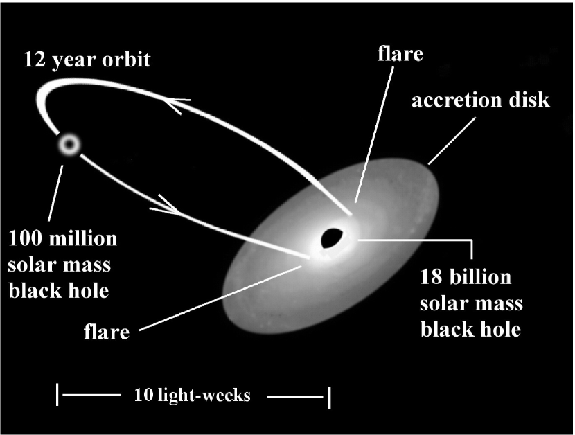
The blazar OJ287 shows an interesting light curve where optical outbursts follow each other in roughly a 12 yr sequence (Sillanpää et al. 1988). The light curve has two significant periodicities, the 12 yr period as well as a 60 yr period (Valtonen et al. 2006a). The simplest explanation of such a doubly periodic system is that it is a binary black hole (BBH) system (Katz 1997) where the accretion disk of the primary is perturbed by a companion on a 12 yr orbit, while the larger period represents a precession cycle. Sundelius et al. (1997) presented a detailed study of this case, and noted that the disk is tidally perturbed during the close encounters. It is reasonable to assume that the tidal perturbations affect the accretion flow, and thus create a 12 yr pattern of increased brightness. The model of Sundelius et al. (1997) is illustrated in Figure 1. The massive central black hole lies in the centre of the accretion disc. The jet emanating from the black hole (not drawn in the figure) is taken to be perpendicular to the disc.

In the BBH model the primary is a massive black hole belonging to the upper end of the black hole mass function (Ghisellini et al. 2009, Sijacki et al. 2009, Kelly et al. 2010, Trakhtenbrot et al. 2011). The host galaxy of OJ287 is bright, $M_{K}\sim-28.9$ (Wright et al. 1998). The primary mass of $1.8\times 10^{10}$ solar mass places OJ287 almost exactly on the black hole mass - host galaxy magnitude relation extended from smaller galaxies and black holes (Kormendy & Bender 2011). The secondary moves in an eccentric orbit of eccentricity $e\sim 0.7$, and it impacts the accretion disc of the primary twice during its 12 yr orbit. The impact points vary from orbit to orbit, and by studying this variation one may determine the rate of the relativistic precession and other parameters of the orbit (Valtonen 2007). The flares arising from disc impacts are easily recognised by the sudden rise of the optical flux and by their generally short duration in comparison with tidal outbursts (Valtonen et al. 2008a, 2009). The mass of the secondary black hole is $\sim 10^{8}$ solar mass, small enough that the accretion disc remains stable in spite of the repeated impacts. The accretion disc is modeled as a magnetic $\alpha_{g}$ disc of Sakimoto & Coroniti (1981). The binary orbit is taken to be nearly perpendicular to the plane of the disc; therefore the jet (not illustrated in Figure 1) lies close to the binary plane.

The future optical light curve of OJ287 was predicted from 1996 to 2030; during the first fifteen years OJ287 has followed the prediction with amazing accuracy, producing five outbursts at expected times, of expected light curve profile and size (Valtonen et al. 2011). In this theory the orbit solution of Lehto $\&$ Valtonen (1996) was used, but because Sundelius et al. (1997) use a ’live’ disc model, the disk is lifted up by the approaching secondary (Ivanov et al. 1998), and the outbursts related to impacts happen earlier than expected in a ’rigid’ disc model. For example, in the ’live’ disc model the 2005 disk impact is about 6 months ahead of the impact in the ’rigid’ disc model, and thus the 2006 April outburst is shifted to 2005 October, as was subsequently observed (Valtonen et al. 2006b,2008b).

In this paper we calculate another property of a ’live’ accretion disc, the change of its orientation as a function of the phase of the binary orbit. Since the changes in the disc orientation are small, Sundelius et al. (1997) did not make an effort to calculate them. The model calculations are then compared with the historical VLBI data of the parsec scale jet orientation as well as with the optical polarization data collected by Villforth et al. (2010), as it is possible that the changing disc orientation is reflected in the orientation of the jet. The jet orientation, in turn, may affect the direction of polarization in the optical emission of the jet.

Figure 1: An illustration of the Sundelius et al. (1997) model. The jet is not shown, but it is taken to lie along the rotation axis of the accretion disc.

2 Optical polarization

In this paper we concentrate on the variation of the position angle of polarization in OJ287, as this is a quantity which may be modeled in the Sundelius et al. (1997) framework. The data have been published and are illustrated in Figure 14 of Villforth et al. (2010). They include data points both from the authors’ own campaign from 2005 to 2009, and earlier measurements. From the point of view of our theory, we are interested in the long term behaviour of the mean polarization angle. Therefore we take averages per each calendar year. They are listed in column 2 of Table 1, together with the standard deviation of the scatter per calendar year in column 3. The last two columns give the number of observations used and the standard error of the mean (Columns 4 and 5, respectively).

Table 1: Mean optical polarization angle and its uncertainty.

Year	Circ PA	STD	N	STD/sqrt(N)
1971	12	22	11	7
1972	87	23	95	2
1973	100	10	33	2
1974	75	7	21	2
1975	85	9	36	1
1976	81	9	20	2
1977	100	10	21	2
1978	78	4	9	1
1979	88	8	23	2
1980	78	3	6	1
1981	134	12	11	4
1982	62	14	35	2
1983	101	17	218	1
1984	145	26	101	3
1985	160	17	14	5
1986	29	26	18	6
1987	100	11	13	3
1988	65	20	33	3
1989	127	7	64	1
1990	114	8	174	1
1991	93	13	129	1
1992	106	3	48	1
1993	62	6	29	1
1994	137	25	105	2
1995	157	22	75	3
1996	176	18	155	1
1997	169	8	95	1
2005	174	15	15	4
2006	171	16	120	1
2007	164	16	129	1
2008	166	21	104	2
2009	170	16	31	3

A few specific points should be noted about the calculation of the average. First, calculating means and standard deviations for directional data can be challenging, especially if the scatter is large. To avoid problems, we use directional statistics for all directional data (Mardia 1975). This is implemented by use of the SciPy module scipy.stats.morestats (www.scipy.org). Second, the individual measurement errors are generally much smaller than the rms scatter. Thus the scatter reflects a genuine variation of the polarization angle, but since our model does not handle short time scale variations, we will not try to model them. Figure 2 shows the resulting mean values as squares and the circular standard deviation as error bars.

Figure 2: The evolution of optical polarization angle in OJ287 together with the circular standard deviation (error bars). Annual mean values are shown.

3 Dynamical model

Our model is the same as in Sundelius et al. (1997) except that the error bars in the orbit model have been recently narrowed down after new outburst timings have been included in the solution (Valtonen et al. 2010a). However, for the purposes of this paper the increased accuracy is of no consequence since the Sundelius et al. (1997) model was already quite accurate. Similarly to Sundelius et al. (1997), the disc of the primary is modeled by non-interacting particles. This limitation is not as bad as it may seem; Sundelius et al. began their simulations with a self-interacting disc, as reported e.g. in Sillanpää et al. (1988), but they soon found out that for the kind of binary orbit considered here, where the disc plane and the orbit plane are perpendicular to each other, the inclusion of self-interaction only increases calculation time greatly without producing significantly different results.

In the present simulation the number of disc particles is 37200. They are placed in circular orbits around the primary, with orbital radii ranging from 8 Schwarzschild radii to 20 Schwarzschild radii of the primary. Varying the inner and outer radii of the disc was not found to influence the result significantly. For every particle, and for every time step, we calculate the orbital elements of the orbits with respect to the primary. The elements are averaged per calendar year. As there are many integration steps per year, typically each annual mean is based on the average of between 2 million and 10 million values. By varying the number of particles it was found that the mean values generated in this way are very robust.

We are interested primarily in the mean orientation of the disc, in the region affected by the secondary. Thus only two orbital elements are of consequence, the inclination of the mean disc $i$ and the corresponding ascending node $\Omega$. The fundamental plane is taken to be the plane of the binary (x-y -plane) at the beginning of the calculation, in year 1856. In the latest orbit model which includes the spin of the primary black hole this plane evolves slowly (Valtonen et al. 2010a). However, the evolution is so slow in the time scale that we are considering that it may be viewed as an invariable plane. The disc is initialized such that the inclinations are typically around $\sim 90^{\circ}$, i.e. particles move in the x-z -plane. For the convenience of discussion, we show in the following figures the quantity $i-\frac{\pi}{2}$ instead of the inclination $i$. The ascending node is measured from a fundamental line (x-axis) in the plane of the binary. The disc is initially loaded such that $\Omega=\pi$, i.e. particles cross the x-y -plane from the underside (negative z-axis) to the upperside (positive z-axis) at the negative x-axis. Figure 3 shows the evolution of these two orbital elements. Here and in the following, $\Omega$ is replaced by $\Omega-\pi$. In practice, the variation of the inclination is very small in comparison with $\Omega$. Why this is so will become clear below (Eqs. 1 & 2).

At this point a free parameter enters our calculation. The sound crossing time of the accretion disc (the region we are considering) is about 10 years. Thus it takes about 10 years to generate physically significant mean values; we do this by taking a sliding average of the surrounding (future and past) values at each annual point. The number of years used in the average is left as a free parameter. In practice we have noticed that taking a sliding mean between 7 and 11 years gives us enough information to see how this free parameter influences our results (see Figure 3).

Figure 3: The evolution of the mean disk in the binary model. The lines with the larger amplitude refer to the ascending node $\Omega-\pi$, with a 7 yr (solid line) and a 10 yr (dashed line) average. The almost constant lines refer to the complement of the inclination $i-\frac{\pi}{2}$.

Figure 3 shows two cycles: a 120 yr precession cycle and the twelve year ’nodding’ cycle. With the sliding mean of 10 years, the 120 yr precession cycle dominates, while going towards the 7 yr sliding average the 12 yr nodding cycle becomes more pronounced. Katz (1997) explained these two frequencies in a physical model. In analogy to Hercules X-1 and SS 433, the precession was attributed to the torque exerted by a companion mass on an accretion disc. Our model is exactly the same, except Katz (1997) chose 12 years and 1.2 years as the periods of the two cycles. However, as mentioned above, in the power spectrum analysis of the light curve of OJ287 the dominant peaks occur at 60 yr and 12 yr (Valtonen et al. 2006a). The observed 60 yr cycle may be only half of the full cycle since Doppler boosting is increased twice during each 120 yr cycle if the viewing angle is small. The model of Katz (1997) is therefore easily applied to the present system. For the increase of cyclic periods by a factor of ten over Katz (1997), and keeping the gravitational radiation lifetime the same, the masses have to be increased by more than an order of magnitude from the $10^{9}$ solar mass scaling by Katz (1997). This fits nicely with the mass scale used in our model where the primary mass is $\sim 1.8\times 10^{10}$ solar mass and the secondary $\sim 1.4\times 10^{8}$ solar mass.

These cycles are also well known in three-body orbit dynamics. In the twice orbit-averaged hierarchical three-body problem the first order equations for the evolution of inclination $i$ and the ascending node $\Omega$ are written

$$\frac{\mathrm{d}i}{\mathrm{d}\tau}=0$$ (1)

$$\frac{\mathrm{d}\Omega}{\mathrm{d}\tau}=-\frac{3}{4}\cos i$$ (2)

(Valtonen & Karttunen 2006) where $\tau$ is the normalized time coordinate,

$$\tau\sim\frac{P}{P_{e}}\frac{t}{P_{e}}$$ (3)

and $t$ is time, and $P$ and $P_{e}$ are the inner and outer periods, respectively. The actual motions are cyclical: the cycle is called the Kozai cycle and its period is $P_{Kozai}\sim 2P_{e}^{2}/P$. For our case $P_{e}\sim 12$ yr, $P\sim P_{e}/5$, and $P_{Kozai}\sim 120$ yr. For inclinations close to $90^{\circ}$, $\cos i\sim\frac{\pi}{2}-i$. The amplitude of the $\Omega$ cycle may be estimated by putting $\mathrm{d}\tau\sim 1$ in Eq. 2; thus the maximal $\mathrm{d}\Omega\sim\frac{\pi}{2}-i$, i.e. it is of the order of one degree in models where the inclination is also within one degree of $90^{\circ}$. Note that the averaging which is done numerically in our simulations is analogous to the analytical orbit averaging in the dynamical theory.

4 The jet

4.1 Modeling the orientation of the optical jet

Presumably the optical emission of OJ287 arises at most times in its jet. Therefore we need to make further assumptions about the disk/jet connection. The disk/jet connection is very much an open problem, and therefore we make a simple assumption: let the jet lie exactly along the rotation axis of the disk and let any bending of the jet be negligible up to parsec scale, i.e. the effect of jet instabilities is omitted here. With this assumption we generate a time sequence of jet orientations from Figure 3. The jet orientation shows up in observations in several ways. First, Doppler boosting generates the base level of optical brightness for OJ287. The 60 yr cycle mentioned earlier may be related to this variation. Thus we take observations from the historical light curve (see e.g. Valtonen et al. 2010b) and remove the well known outburst peaks. The resulting base level light curve is shown in Figure 4. In generating this light curve the highest optical V-magnitude was selected from each 0.1 yr interval of time.

Figure 4: The variation of the base level brightness in OJ287. The V-magnitudes are the minimum measured values per 0.1 yr time interval. Curves represent the effects of Doppler boosting on the base level magnitude.

Figure 4 has also two lines representing the effect of the Doppler boosting on the optical brightness, vertically displaced by about two magnitudes, which are generated using the data in Figure 3. In order to carry out the transformation from Figure 3 to Figure 4 it is necessary to adopt four free parameters: two parameters of the viewing angle of the observer, the Lorentz factor $\Gamma$ in the jet, and the time delay between the instantaneous change of the disk plane and the transmission of this information to the central axis and the jet. The values for the parameters are obtained by fitting the curves to the range of data points in Figure 4.

In order to calculate the viewing angle, we parameterize the plane perpendicular to the line of sight by the same two angles, inclination $i_{0}$ and ascending node $\Omega_{0}$, as those used to describe the disk plane. Thus the direction to the observer is represented by two horizontal lines in Figure 3. For any moment of time we measure the vertical distance between the line $\Omega_{0}-\pi$ and the $\Omega-\pi$ curve as well as the distance of the $i_{0}-\frac{\pi}{2}$ line and the $i-\frac{\pi}{2}$ curve. This gives us the two components of the viewing angle as a function of time. The $i-\frac{\pi}{2}$ component of the viewing angle is practically constant. In this way we generate sets of viewing angles as a function of time, and shift them forward by some value $\Delta t$ which should be of the order of the sound crossing time in the disk. For each moment of time we may then calculate the Doppler boosting factor, assuming some value of $\Gamma$.

In order to produce a 60 yr periodic component out of the basic 120 yr cycle, we need to choose the viewing angle so that $\Omega_{0}$ is inside the variability range of $\Omega$ in Figure 3. The curves in Figure 4 are based on $\Omega_{0}-\pi=0^{\circ}.4$, $i_{0}-\frac{\pi}{2}=-0^{\circ}.4$, $\Delta t=13$ yr and $\Gamma=30$. This fit does not take into account other factors besides the steady jet contributing to the optical brightness. Thus the value of $\Gamma$ is only indicative of the general magnitude of the Lorentz factor; it is not significantly different from the values obtained by other means ($\Gamma\sim 20$, Jorstad et al. 2005). Our range of viewing angles is between $1^{\circ}$ and $2^{\circ}$, again in agreement with findings in other studies (Lähteenmäki and Valtaoja 1999, Jorstad et al. 2005, Savolainen et al. 2010).

4.2 Orientation of the VLBI jet

Table 2: Historical data showing the mean direction of OJ 287’s VLBI jet within the first 1 mas from the core. The full table is available as Supporting Information with the online version of this article.

Obs. Date	Arraya	$\lambda$	PA	$\Delta$PAb	Ref.c
(yr)		(cm)	(deg)	(deg)
1981.95	USVN	6	-116	…	1
1982.95	USVN	6	-113	…	1
1985.51	Geo	3.6	-82	3	2
1985.75	Geo	3.6	-83	3	2
1985.89	Geo	3.6	-93	3	2
1986.27	Geo	3.6	-103	5	2
1986.50	Global	6	-100	…	3

The second way to measure the jet rotation is to look at its position angle in the sky. Unfortunately it is impossible to resolve the optical jet, but at radio wavelengths the jet is observable in parsec scale with the VLBI and its orientation is known since the early 1980s.

We have constructed the observed history of variations in the position angle of OJ287’s radio jet by collecting the available VLBI data from the literature. The jet PA was defined as the mean PA within the first one milliarcsecond (mas) from the VLBI core, which is the bright feature at one end of the jet. The mean PA was measured by fitting an ordinary-least-squares bisector regression line to the jet component positions if more than one such component was present within 1 mas from the core. The regression line was forced to go through the core position and the each component was assigned a positional uncertainty equivalent to 10% of the component’s size convolved with the beam size (see Lister et al. 2009a). In the least-squares fit the data points were weighted by the inverse square of their positional uncertainty times the component’s (normalized) flux density. If only one component was present within 1 mas from the core, the PA of this knot was assumed as the jet PA. Table 2 lists 140 individual jet PA measurements obtained in this manner and covering a time period from 1981 to 2009. These observations were made at 2, 3.6, and 6 cm wavelengths. We chose these wavelengths because within this range the jet PA seems to be very weakly wavelength-dependent, and because there are abundant historical data available through the geodetic observations (3.6 cm) and the VLBA 2 cm / MOJAVE Surveys (Kellermann et al. 1998,Lister et al. 2009a). We did not try to back-extrapolate the ejection epochs of the knots, since it easily leads to ambiguous results for inhomogeneous data sets with time gaps. The proper motions close to the core in OJ287 are $\sim 0.5-0.8$ mas yr^-1 meaning that we measure the changes in the PA with a delay of $\sim 1-2$ yr (Lister et al. 2009a).

Figure 5 presents the long-term evolution of the VLBI jet’s position angle. The values there are weighted annual means of $2-6$ cm measurements. The error bars represent either the standard deviation of the scatter in a given year (multiple observations per year) or the uncertainty of a single measurement. As mentioned earlier, stacking 2, 3.6, and 6 cm data together does not add a bias to the PA curve, since the average difference in (quasi-)simultaneously measured PAs between these wavelengths is close to zero.

The projected jet PA presented in Figure 5 varies with a total amplitude of $\sim 50$ degrees, it has an overall decreasing trend, and it shows two significant “spikes” separated by about a decade. Tateyama & Kingham 2004 have earlier reported a varying jet PA in OJ287 and proposed that this may be due to the precession of a ballistic jet. Comparison of Figure 5 to Figure 6 in Tateyama & Kingham (2004) shows, however, that this specific periodic model does not fit the observed variations in jet PA when data spanning three decades is considered. Moor et al. (2011) show another recent compilation of the PA data with a 12 yr cyclic structure together with the overall long term trend.

Figure 5: The variation of the position angle of the parsec scale radio jet in the sky. Squares are annual averages, and the error bars represent uncertainties. The dashed line refers to the model with a 10 yr average and $\Delta t=13$ yr. If $\Delta t=4$ yr, as discussed in the text, then the model line is moved backward, and after a slight adjustment of the vertical scale, is shown as a solid line.

The lines in Figure 5 are the projected position angles in the sky calculated from our model. They have been drawn for the same parameter values as the lines in Figure 4, except that for the solid line the time delay $\Delta t$ is only 4 years. The free parameters here are the time delay and the zero point of the projected jet orientation. The 13 yr time delay model and the PA measurements agree in general outline, with the exception of the two earliest data points, which are from four-station experiments with the U.S. VLBI array. The poor $(u,v)$ coverage of these observations leaves the jet orientation more uncertain than in the rest of the data.

The model predicts that the jet PA should rapidly turn clockwise by $\sim 50$ degrees within the next ten years. Also, the model is coming to a minimum in the angle between the jet and our line-of-sight. As the viewing angle approaches the half-opening angle of the jet, the appearance of the VLBI jet can change significantly: the apparent opening angle increases, any bending is exacerbated, and differential Doppler boosting may affect the observed structure. Based on a sequence of 7 mm VLBA images Agudo et al. (2010,2011) recently reported a greatly changed PA in the innermost part of OJ287’s jet during 2008–2010. They gave a new jet PA of $\sim-200^{\circ}$ or $\sim-20^{\circ}$, depending on the identification of the core component. Agudo et al. (2010) propose that the jet is indeed crossing our line-of-sight and the sudden change in the PA may be due to a moving kink in the jet with an almost zero viewing angle. One cannot, however, directly compare the PA values reported by them with those presented in Figure 5, since the PAs given in Agudo et al. (2010,2011) refer to the mutual orientation of the two innermost bright features at 7 mm that are separated by only $\sim 0.2$ mas, whereas the PAs shown in Figure 5 refer to the mean orientation of the jet within the first 1 mas in the 2-6 cm images. Therefore, further VLBI observations are needed to test if the predicted change in the jet orientation takes place.

If the time delay turns out to be shorter than in the optical variations, it may imply that the information on the change of jet orientation is transmitted to the axis via the hot corona surrounding the accretion disk, with a speed of sound (actually, Alfven speed) which is much greater than the sound speed in the disk. The value of $\Gamma$ does not enter this calculation.

5 Optical polarization angle

In the following we make the simplifying assumption that the symmetry axis of the magnetic field structure in the jet is at a constant angle relative to the jet axis. This basically requires either a reasonably stable vector-ordered magnetic field in the jet or a long-lived stationary shock in the region where the optical emission originates. Thus when the jet points in different directions, so does the electric field vector of the oscillating electrons. Consider first the case where the electric field vector is almost parallel to the jet. The electric field vector has its own viewing angle which is in general different from the viewing angle of the jet. Let the plane which is perpendicular to the electric field vector be specified by angles $\Omega_{1}$ and $i_{1}$. We will now consider determining these parameters when $\Delta t=13$ yr in the optical part of the jet.

Figure 6 shows the polarization angle data together with a fit to a model with $\Omega_{1}-\pi=1^{\circ}.6$ and $i_{1}-\frac{\pi}{2}=0^{\circ}.25$. This means that the jet and the electric field vector are at an angle of $1^{\circ}.4$ relative to each other. An almost parallel EVPA with respect to the jet axis could be generated by a large-scale helical magnetic field with a dominant toroidal component or a compressed magnetic field of a long-lived (oblique) standing shock front in the jet (see Lyutikov et al. 2005 for a discussion of jet polarization).

However, there is a $90^{\circ}$ shift in the PA given by this model with respect to the best fit with observations. This leads us to another possibility, namely that the poloidal magnetic field component dominates in the section of the jet where the optical emission comes from. In that case the PA that we are plotting is the direction of the magnetic field, with a small but significant deviation from the jet line. Then we should add $90^{\circ}$ to the PA values in our model in order to compare with the observed polarization angle (Laing 1981, Lyutikov et al. 2005). It is not possible to decide $\it{apriori}$ which case we should have in OJ287 since it depends sensitively on the physical structure of the jet. However, it is generally thought that the optical emission arises rather close to the central engine (e.g. Agudo et al. 2011). Since the poloidal magnetic field component increases faster than the toroidal field component towards the centre, it is likely that in our case the poloidal field should dominate, and we should add $90^{\circ}$ to the PA values, as we do in Figure 6.

We notice that the model describes well the general feature of the polarization angle evolution, noticed by Villforth et al. (2010), that the position angle has changed in an almost steplike fashion from $\sim-90^{\circ}$ to $\sim 0^{\circ}$ in the early 1990’s. The prediction of the model is that this position angle should hold on during the coming decades. Note that the model assumes optically thin conditions in the jet and thus the $90^{\circ}$ jump in PA around 1995 has nothing to do with the changes in optical depth. Neither do we need a dramatic change of the magnetic field configuration in the jet at that time, as suggested by Villforth et al. (2010). Quite opposite, our model assumes a constancy of the jet, and looks only at the PA changes due to the changing viewing angle.

In some years the theoretical line goes well outside the error range of the annual average. We should note that especially in mid 1980’s the PA varied over the whole angular range even in one year (see Figure 14 of Villforth et al 2010), and the calculation of the average value is very sensitive to the $\pm 180^{\circ}$ ambiguity in the observed polarization angles. For example, by a different choice of the quadrant for just one or two observations, the position angles $100^{\circ}$ in 1971, $116^{\circ}$ in 1984, $95^{\circ}$ in 1985, $90^{\circ}$ in 1986 and $102^{\circ}$ in 1994 can also be found. In all of these cases the correction goes to the direction of improving the fit with the theoretical line. However, for the other years such uncertainty does not exits, and the remaining difference with the theory must be considered real. We have also broken down the data in semi-annual boxes, but it does not help to clarify the situation with respect to the most uncertain points.

Figure 6: The evolution of the optical polarization angle compared with the model. The curves are for a 10 yr (dash-dot line) and for an 11 yr (dashed line) average. Observations refer to the values in Table 1 minus $180^{\circ}$. The theoretical lines are shifted by adding $90^{\circ}$; there is a $90^{\circ}$ uncertainty in the polarization angle due to unknown physical conditions in the jet (Lyutikov et al. 2005).

6 Conclusions

Using a number of simplifying assumptions, we have calculated how the orientation of OJ287’s relativistic jet is expected to vary in the binary black hole model of Sundelius et al. (1997). Even though the model does not include a detailed physical treatment of the jet/disk connection, it agrees with the observed radio jet orientation as well as optical polarization evolution of OJ287 in general outline. The scatter in the polarization position angle is large which makes a very specific comparison difficult.

The view which we have arrived at is that in many respects OJ287 can be modeled as a binary system, a scaled up version of Her X-1 or SS433. In the presented model of OJ287, the jet sweeps across the line of sight in a periodic manner, and this motion creates brightness variations by varying Doppler boosting as well as shows up as a varying projection of the jet. While the projected radio jet is actually observed, in optical we gain evidence of the beam sweeping by the varying optical polarization angle. When the analytical model of Katz (1997) is scaled up for the observed cycle frequencies, it explains well the numerical simulation results of this work. The presented model makes predictions about the future trends of the observables discussed in this paper and therefore it can be easily further tested by continuing the VLBI and polarization monitoring of OJ287.

References

- Agudo et al. (2010) Agudo, I. et al. 2010, in Fermi meets Jansky - AGN in radio and gamma-rays, eds. T. Savolainen et al., p. 143.
- Agudo et al. (2011) Agudo, I. et al. 2011, ApJ, 726, L13
- Fey et al. (1996) Fey, A.L. et al. 1996, ApJS, 105, 299
- Fey & Charlot (1997) Fey, A.L. & Charlot, P. 1997, ApJS, 111, 95
- Gabuzda et al. (1989) Gabuzda, D.C., Wardle, J.F.C., & Roberts, D.H. 1989, ApJ, 336, 59
- Gabuzda & Cawthorne (1996) Gabuzda, D.C. & Cawthorne, T.V. 1996, MNRAS, 283, 759
- Gabuzda & Gomez (2001) Gabuzda, D.C. & Gomez, J.L. 2001, MNRAS, 320, 49
- Ghisellini et al. (2009) Ghisellini, G., Foschini, L., Volonteri, M., Ghirlanda, G., Haardt, F., Burlon, D. & Tavecchio, F. 2009, MNRAS, 399, L24
- Ivanov et al. (1998) Ivanov, P.B., Igumenshchev, I.V. & Novikov, I.D. 1998, ApJ, 507, 131
- Jorstad et al. (2001) Jorstad, S.G. et al. 2001, ApJS, 134, 181
- Jorstad et al. (2005) Jorstad, S.G. et al. 2005, AJ, 130, 1418
- Katz (1997) Katz, J. I. 1997, ApJ, 478, 527
- Kellermann et al. (1998) Kellermann, K.I., Vermeulen, R.C., Zensus, J.A. & Cohen, M.H. 1998, AJ, 115, 1295
- Kelly et al. (2010) Kelly, B., Vestergaard, M., Fan, X., Hopkins, P., Hernquist, L. & Siemiginowska, A. 2010, ApJ, 719, 1315
- Kormendy et al. (2011) Kormendy, J. & Bender, R. 2011, Nature, 469, 377
- Lähteenmäki et al. (1999) Lähteenmäki, A. & Valtaoja, E. 1999, ApJ, 521, 493
- Laing (1981) Laing, R.A. 1981, ApJ, 248, 87
- Lehto & Valtonen (1996) Lehto, H.J., & Valtonen, M.J. 1996, ApJ, 460, 207
- Lister et al. (2009a) Lister, M.L. et al. 2009, AJ, 137, 3718
- Lister et al. (2009b) Lister, M.L. et al. 2009, AJ, 138, 1874
- Lyutikov et al. (2005) Lyutikov, M., Pariev, V.I. & Gabuzda, D. C. 2005, MNRAS, 360, 869
- Mardia (1975) Mardia, K.V. 1975, JRStatSoc, SerB, 37, 349
- Moor et al. (2011) Moor, A., Frey, S., Lambert, S. B., Titov, O. A. & Bakos, J. 2011, AJ, 141, 178
- Ojha et al. (2004) Ojha, R. et al. 2004, ApJS, 150, 187
- Piner et al. (2007) Piner, B.G, Mahmud, M., Fey, A.L., & Gospodinova, K. 2007, AJ, 133, 2357
- Roberts et al. (1987) Roberts, D.H., Gabuzda, D.C., & Wardle, J.F.C. 1987, ApJ, 323, 536
- Savolainen et al. (2010) Savolainen, T. et al. 2010, A&A, 512, A24
- Sijacki et al. (2009) Sijacki, D., Springel, V. & Haehnelt, M.G. 2009, MNRAS, 400, 100
- Sillanpää et al. (1988) Sillanpää, A., Haarala, S., Valtonen, M.J., Sundelius, B. & Byrd, G.G. 1988, ApJ, 325, 628
- Sakimoto & Coroniti (1981) Sakimoto, P.J. & Coroniti, F.V. 1981, ApJ, 247, 19
- Sundelius et al. (1997) Sundelius, B., Wahde, M., Lehto, H.J. & Valtonen, M.J., 1997, ApJ, 484, 180
- Tateyama et al. (1999) Tateyama, C.E. et al. 1999, ApJ, 520, 627
- Tateyama & Kingham (2004) Tateyama, C.E. & Kingham, K.A. 2004, ApJ, 608, 149
- Trakhtenbrot et al. (2011) Trakhtenbrot, B., Netzer, H., Lira, P. & Shemmer, O. 2004, ApJ, 730, 7
- Valtonen & Karttunen (2006) Valtonen, M.J., & Karttunen, H. 2006, The Three Body Problem, Cambridge UP, Cambridge, p. 233
- Valtonen et al. (2006a) Valtonen, M.J. et al. 2006a, ApJ, 646, 36
- Valtonen et al. (2006b) Valtonen, M.J., Nilsson, K., Sillanpää, A., Takalo, L.O., Lehto, H.J., Keel, W.C., Haque, S., Cornwall, D. & Mattingly, A. 2006b, ApJ, 643, L9
- Valtonen (2007) Valtonen, M.J. 2007, ApJ, 659, 1074
- Valtonen et al. (2008a) Valtonen, M.J. et al. 2008a, Nature, 452, 851
- Valtonen et al. (2008b) Valtonen, M., Kidger, M., Lehto, H. & Poyner, G. 2008b, A&A, 477, 407
- Valtonen et al. (2009) Valtonen, M.J. 2009, ApJ, 698, 781
- Valtonen et al. (2010a) Valtonen, M.J. et al. 2010a, ApJ, 709, 725
- Valtonen et al. (2010b) Valtonen, M.J. et al. 2010b, CeMDA, 106, 235
- Valtonen et al. (2011) Valtonen, M.J., Lehto, H.J., Takalo, L.O. & Sillanpää, A. 2011, ApJ, 729, 33
- Vicente et al. (1996) Vicente, L., Charlot, P., & Sol, H. 1996, A&A, 312, 727
- Villforth et al. (2010) Villforth, C. et al. 2010, MNRAS, 402, 2087
- Wright et al. (1998) Wright, S.C., McHardy, I.M. & Abraham, R.G. 1998, MNRAS, 295, 799