Finite-temperature phase diagram of two-component bosons in a cubic optical lattice: Three-dimensional $t$-$J$ model of hard-core bosons

Abstract

We study the three-dimensional bosonic $t$-$J$ model, i.e., the $t$-$J$ model of “bosonic electrons”, at finite temperatures. This model describes the $s={1\over 2}$ Heisenberg spin model with the anisotropic exchange coupling $J_{\bot}=-\alpha J_{z}$ and doped bosonic holes, which is an effective system of the Bose-Hubbard model with strong repulsions. The bosonic “electron” operator $B_{r\sigma}$ at the site $r$ with a two-component (pseudo-)spin $\sigma(=1,2)$ is treated as a hard-core boson operator, and represented by a composite of two slave particles; a “spinon” described by a Schwinger boson (CP¹ boson) $z_{r\sigma}$ and a “holon” described by a hard-core-boson field $\phi_{r}$ as $B_{r\sigma}=\phi^{\dagger}_{r}z_{r\sigma}$. By means of Monte Carlo simulations, we study its finite-temperature phase structure including the $\alpha$ dependence, the possible phenomena like appearance of checkerboard long-range order, super-counterflow, superfluid, and phase separation, etc. The obtained results may be taken as predictions about experiments of two-component cold bosonic atoms in the cubic optical lattice.

I Introduction

Cold-atomic systems are one of the most intensively studied topics not only in atomic physics but also in condensed matter physics in these days. In particular, cold atoms put on an optical lattice (OL) may be used as a “simulator” to study certain canonical models of strongly-correlated electron systemsoptical . For systems in the OL, interactions between atoms, dimensionality of system, etc. are highly controllable, and effects of impurities are strongly suppressed. Therefore, cold atomic systems in the OL are sometimes called final simulators. Among them, systems of double-species atoms are quite interesting from the view point of the high-temperature ($T$) superconductivity (SC). Investigation of these atomic systems is expected to give an important insight into mechanism of SC in systems in which only repulsive interactions between particles exist.

In this paper, we shall study the $t$-$J$ model of hard-core bosons in the cubic lattice. There are (at least) two versions of the bosonic $t$-$J$ modelBtJ1 . In the previous paperBtJ1 , we studied one version that is a bosonic counterpart of the original fermionic $t$-$J$ model and respects the SU(2) spin symmetry. On the other hand, in the present paper, we shall consider the second version that is an effective model of the two-band Bose-Hubbard model with strong repulsions and the total filling factor not exceeding unityBtJ2 . Relation and differences between these two versions of the bosonic $t$-$J$ model were explained in the previous paperBtJ1 . Obtained results for the second version of the $t$-$J$ model in the present paper can be regarded as predictions about the system of bosonic atoms of two-species. Related Hubbard model at commensurate fillings has been studied in e.g., Ref.altman by the mean-field-theory (MFT) type approximation, and its one-dimensional counterpart by the Tomonaga-Luttinger liquid theory in Ref.Hu . In the present paper, we shall study the three-dimensional (3D) $t$-$J$ model at fractional fillings mostly by means of the Monte-Carlo (MC) simulations. Results are compared with the ones obtained previously.

The paper is organized as follows. In Sect.2 we explain the model and its basic properties. We also study it by MFT briefly. In Sect.3 we present the results of MC simulations. Section 4 is devoted for conclusions and discussions.

II Model

II.1 The $t$-$J$ model

The $t$-$J$ model is derived from the Bose-Hubbard modelBHM whose Hamiltonian is given as

$$H_{\rm Hub} = \sum_{r}\Big{[}-t\sum_{i=1}^{3}(a^{\dagger}_{r+i}a_{r}+b^{\dagger}_{r+i}b_{r}+\mbox{h.c.})+Un_{ar}n_{br}$$ (2.1)

$$+{V\over 2}\sum_{\lambda=a,b}n_{\lambda r}(n_{\lambda r}-1)-\mu_{c}\sum_{\lambda=a,b}n_{\lambda r}\Big{]},$$

where $r$ denotes site of the cubic lattice, $i(=1,2,3)$ is the unit vector in the $i$-th direction (it also denotes the direction index), and $a_{r}$ and $b_{r}$ are boson annihilation operators. $n_{\lambda}$ is the number operator of the boson $\lambda$, and therefore $U$ and $V$ are inter- and intra-species interactions, respectively. This $H_{\rm Hub}$ describes the system of two-species of cold bosonic atoms in a cubic OL. From Eq.(2.1), it is obvious that $a$ and $b$ atoms have the same hopping amplitude and the same density $\rho_{a}=\rho_{b}$ in the present system. Recently studied ⁸⁵Rb -⁸⁷Rb atomic system2BEC is a typical example described by this Hamiltonian.

Some related models to $H_{\rm Hub}$ in Eq.(2.1) have been studied so far. In the present paper, we consider the specific case such that $t\ll U,V$ and the total number of bosons at each site is not exceeding unity $(0\leq n_{ar}+n_{br}\leq 1$). It is obvious that the model in the above parameter region is closely related with the high-$T_{\rm c}$ materials and therefore it is expected that study on it gives rise to an important insight into the physical properties of the high-$T_{\rm c}$ materials. It should be remarked that at present the properties of the fermionic $t$-$J$ model are poorly understood in spite of the quite intensive studies on it for more than two decades. This fact mainly stems from the difficulties of numerical study on fermionic systems.

The effective Hamiltonian in the large on-site repulsion limit can be derived by the standard methods of expansion in powers of $t/U,t/V$effectiveH as follows;

$$H_{tJ} = -t\sum_{r,i=1}^{3}(a^{\dagger}_{r+i}a_{r}+b^{\dagger}_{r+i}b_{r}+\mbox{h.c.})+J_{z}\sum_{r,i}S^{z}_{r+i}S^{z}_{r}$$

$$-J_{\bot}\sum_{r,i}(S^{x}_{r+i}S^{x}_{r}+S^{y}_{r+i}S^{y}_{r})-\bar{\mu}_{c}\sum_{r}(1-n_{ar}-n_{br}),$$

where the SU(2) pseudo-spin operator is given as $\vec{S}_{r}={1\over 2}B^{\dagger}_{r}\vec{\sigma}B_{r}$ with $B_{r}=(a_{r},b_{r})^{t}$ ($\vec{\sigma}$ is the Pauli spin matrices). The exchange couplings are

$$J_{z}={4t^{2}\over U}-{4t^{2}\over V}+\cdots,\ J_{\bot}={2t^{2}\over U}+\cdots,\ J_{\bot}=-\alpha J_{z},$$ (2.3)

and $\bar{\mu}_{c}$ is the chemical potential of holes. In the following discussion, we shall treat $t,\;J_{z}$ and $J_{\bot}$, hence $\alpha$, as free parameters, and study the $t$-$J$ model (LABEL:HtJ). After obtaining the critical couplings etc, we shall return to the expression (2.3).

II.2 Physical-state condition: Double-CP¹ representation

In the system of $H_{tJ}$ in Eq.(LABEL:HtJ), a physical state at each site $r$ is expanded by three orthogonal basis state vectors $\{|0\rangle,|a\rangle=a^{\dagger}_{r}|0\rangle,|b\rangle=b^{\dagger}_{r}|0\rangle\}\ (a_{r}|0\rangle=b_{r}|0\rangle=0)$. In order to express this constrained Hilbert space faithfully, we use the following slave-particle representation,

$$a_{r}=\phi^{\dagger}_{r}c_{r1},\;\;\;b_{r}=\phi^{\dagger}_{r}c_{r2},$$ (2.4)

$$\Big{(}\phi^{\dagger}_{r}\phi_{r}+c^{\dagger}_{r1}c_{r1}+c^{\dagger}_{r2}c_{r2}-1\Big{)}|\mbox{phys}\rangle=0,$$ (2.5)

where $\phi_{r}$ is a hard-core boson and $c_{r\sigma}\ (\sigma=1,2)$ is an ordinary boson. The three basis states are expressed in terms of $c_{r\sigma}$ and $|\Omega\rangle\ (c_{r\sigma}|\Omega\rangle=0)$ as

$$|0\rangle\leftrightarrow\phi^{\dagger}_{r}|\Omega\rangle,\;\;a^{\dagger}_{r}|0\rangle\leftrightarrow c^{\dagger}_{r1}|\Omega\rangle,\;\;b^{\dagger}_{r}|0\rangle\leftrightarrow c^{\dagger}_{r2}|\Omega\rangle.$$ (2.6)

In order to express the local constraint (2.5) in more convenient way, we introduce a CP¹ boson (Schwinger boson) $z_{r\sigma}$,

$$c_{r\sigma}=(1-\phi^{\dagger}_{r}\phi_{r})z_{r\sigma},\;\;(\sigma=1,2)$$

$$\Big{(}\sum_{\sigma=1,2}z^{\dagger}_{r\sigma}z_{r\sigma}-1\Big{)}|\mbox{phys}\rangle_{z}=0.$$ (2.7)

It is easily verified that Eq.(2.5) is satisfied by Eq.(2.7).

The hard-core boson $\phi_{r}$ itself can be expressed in terms of another CP¹ boson $w_{rf}$ as followsBtJ1 ,

$$\phi_{r}=w^{\dagger}_{r2}w_{r1},\;\;\Big{(}\sum_{f=1,2}w^{\dagger}_{rf}w_{rf}-1\Big{)}|\mbox{phys}\rangle_{w}=0.$$ (2.8)

From Eq.(2.8), it is obvious that $|0\rangle_{\phi}=w^{\dagger}_{r2}|0\rangle_{w}$ and $\phi^{\dagger}_{r}|0\rangle_{\phi}=w^{\dagger}_{r1}|0\rangle_{w}$, where $|0\rangle_{\phi}(|0\rangle_{w})$ is the empty state of $\phi_{r}(w_{r})$. It is straightforward to verify that $\phi_{r}$ satisfies the mixed commutation relations of hard-core bosonsBtJ1 . Then the Hamiltonian $H_{tJ}$ can be expressed in terms of the two sets of CP¹ bosons $z_{r\sigma}$ and $w_{rf}$. The partition function $Z$ at finite $T$ is given by the path-integral as

$$Z=\int[DwDz]\exp[-\int_{0}^{\beta}d\tau(\bar{z}\dot{z}+\bar{w}\dot{w}+H_{tJ}(\bar{w},w,\bar{z},z))],$$ (2.9)

where $\tau$ is the imaginary time, $\beta=1/(k_{\rm B}T)$ and $H_{tJ}(\bar{w},w,\bar{z},z)$ is obtained from $H_{tJ}$ in (LABEL:HtJ) by substituting the double-CP¹ representation for $a_{r}$ and $b_{r}$. In the present numerical study, we ignore the $\tau$-dependence of $z(\tau)$ and $w(\tau)$ and consider the following system,

$$Z^{\prime}=\int[DwDz]\exp[-\beta H_{tJ}(\bar{w},w,\bar{z},z)],$$ (2.10)

where $z$ and $w$ represent the zero-modes of $z(\tau)$ and $w(\tau)$. This approximation is justified when we consider system at sufficiently high temperature. However, we expect that the system (2.10) has at least qualitatively the same phase structure to that of (2.9) for $T>0$. As we discussed in Ref.BtJ1 , the nonzero-modes of $z(\tau)$ and $w(\tau)$ renormalize $H_{tJ}$ and this renormalization tends to order the system. Therefore it is expected that ordered phase found in the system (2.10) also exists in the system (2.9). This expectation was actually verified in some systemssawa .

II.3 Mean-field theory

Before going into the details of numerical study of Eq.(2.10), it is useful to investigate the ground-state properties of the model by the MFT. We use a variational wave function of bosons $a_{r}$ and $b_{r}$ that has a site-factorized form,

$$|\Psi\rangle=\prod_{r}\Big{[}\sin{\theta_{r}\over 2}\Big{(}\sin{\chi_{r}\over 2}a^{\dagger}_{r}+\cos{\chi_{r}\over 2}b^{\dagger}_{r}\Big{)}+\cos{\theta_{r}\over 2}\Big{]}|0\rangle.$$ (2.11)

Here we assume the sublattice symmetry and put $\theta_{r}=\theta$, $\chi_{r}=\chi_{\rm A(B)}\ [r\in\mbox{A(B)-sublattice}]$. Then the mean-field energy ${\cal E}_{tJ}$ is given as

$${{\cal E}_{tJ}\over N_{L}} = -{t\over 2}\sin^{2}\theta\Big{(}\sin{\chi_{\rm A}\over 2}\sin{\chi_{\rm B}\over 2}+\cos{\chi_{\rm A}\over 2}\cos{\chi_{\rm B}\over 2}\Big{)}$$ (2.12)

$$+{J_{z}\over 4}\sin^{4}{\theta\over 2}\cos\chi_{\rm A}\cos\chi_{\rm B}-{J_{\bot}\over 4}\sin^{4}{\theta\over 2}\sin\chi_{\rm A}\sin\chi_{\rm B}$$

$$-\bar{\mu}_{c}\cos^{2}{\theta\over 2},$$

where $N_{L}$ is the number of links in the system. By minimizing ${\cal E}_{tJ}$, we can obtain the MF phase diagram. The case in which the filling is unity, $n_{ra}+n_{rb}=1$, corresponds to $\theta=\pi$ in (2.11), and

$${{\cal E}_{tJ}\over N_{L}}\Big{|}_{\theta=\pi}={J_{z}\over 4}\cos\chi_{\rm A}\cos\chi_{\rm B}-{J_{\bot}\over 4}\sin\chi_{\rm A}\sin\chi_{\rm B}.$$ (2.13)

The lowest-energy state there is easily obtained as

$$\mbox{For}\;J_{z}>J_{\bot},\;\;(\chi_{\rm A},\chi_{\rm B})=(0,\pi),\;\;\mbox{or}\;\;(\chi_{\rm A},\chi_{\rm B})=(\pi,0),$$

$$\mbox{For}\;J_{\bot}>J_{z}>-J_{\bot},\;\;(\chi_{\rm A},\chi_{\rm B})=\Big{(}{\pi\over 2},{\pi\over 2}\Big{)}.$$ (2.14)

Then for $J_{z}>J_{\bot}$, the lowest-energy state is the checkerboard state of particle $a$ and $b$, whereas for $J_{\bot}>J_{z}$ the state of super-counter-flow (SCF) $\langle a^{\dagger}_{r}b_{r}\rangle\neq 0$ is realized as expected. The checkerboard state corresponds to an antiferromagnetic (AF) state, whereas the SCF corresponds to a XY-ferromagnetic state in the magnetism terminology.

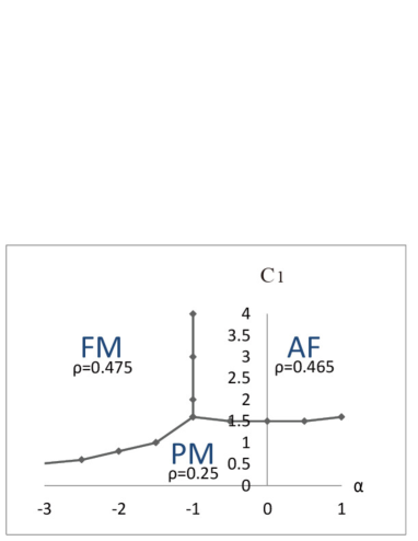
Figure 1: Phase structure for $t=0$ and $\bar{\mu}_{c}=0$ in the $\alpha-c_{1}$ plane, where $\alpha=-J_{\bot}/J_{z}$ and $c_{1}=\beta J_{z}$. There are three phases and their physical meaning is explained in the text. Typical value of $\rho=\langle a^{\dagger}_{r}a_{r}\rangle=\langle b^{\dagger}_{r}b_{r}\rangle$ in each phase is also shown.

Doping holes shifts $\theta$ to $\theta<\pi$. From Eq.(2.12), the lowest-energy state is obtained as

$${\rm For}\ J_{\bot}>J_{z},\chi_{\rm A}=\chi_{\rm B}={\pi\over 2},$$

$${\rm For}\ J_{z}>J_{\bot},\chi_{\rm A}(\chi_{\rm B})=\epsilon,\;\chi_{\rm B}(\chi_{\rm A})=\pi-\epsilon,$$

$$\epsilon\equiv{4t\over J_{z}-J_{\bot}}\cos^{2}{\theta\over 2}={4t\over J_{z}-J_{\bot}}(1-n_{a}-n_{b}).$$ (2.15)

Thus, for $J_{\bot}>J_{z}$ Bose-Einstein condensation (BEC) of both $a$ and $b$ atoms occurs in addition to the SCF. On the other hand, for $J_{z}>J_{\bot}$, superfluidity (SF) with checkerboard symmetry, so called supersolid (SS), appears for an arbitrary small but finite value of $t$ and the hole densitySS . However, this result by the MFT is not reliable even for the present three-dimensional system because fluctuations of the relative phases of $|0\rangle,\;a^{\dagger}_{r}|0\rangle$ and $b^{\dagger}_{r}|0\rangle$ have been ignored in the MFT.

In the following section, we shall study the model by means of the MC simulations. The numerical study gives reliable result for the phase structure of the model and also details of its critical behavior.

III Results of MC simulations

III.1 Case of $t=0$

Let us turn to the numerical studyMC . We conisder the cubic lattice with its linear size $L$ up to 20 and impose the periodic boundary condition. In order to find phase transition lines, we calculate the internal energy $U$ and the specific heat $C$ defined as

$$U=\frac{1}{N}\langle H_{tJ}\rangle,\ C=\frac{1}{N}\langle(H_{tJ}-U)^{2}\rangle,\ N\equiv L^{3}.$$ (3.1)

Furthermore we calculate various correlation functions to identify each observed phase.

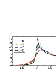
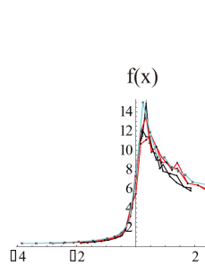
Figure 2: (Left) $C$ at $t=0$ as a function of $c_{1}$ for $\alpha=-0.5$. It indicates the existence of a second-order phase transition (PM $\rightarrow$ AF) at $c_{1}\simeq 1.51$. (Right) The scaling function $f(x)$ for $C$ obtained by finite-size scaling (FSS) hypothesisFSS . The critical exponent of the correlation length is $\nu=0.70$.

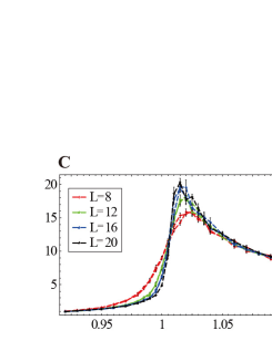
Figure 3: (Left) $C$ as a function of $c_{1}$ for $\alpha=-1.5$. Result indicates the existence of second-order phase transition (PM $\rightarrow$ FM) at $c_{1}\simeq 1.015$. (Right) Scaling function $f(x)$. Critical exponent is obtained as $\nu=1.0$.

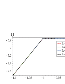
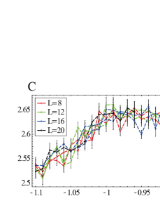
Figure 4: $U$ and $C$ at $t=0$ as a function of $\alpha$ for $c_{1}=3$. Phase transition takes place at $\alpha\simeq-1.0$.

It is convenient to use the following parameterization,

$$\alpha=-\frac{J_{\bot}}{J_{z}},\ c_{1}=\beta J_{z},\ c_{3}=\beta t.$$ (3.2)

We first consider the case of vanishing hole hopping, i.e., $t=0$. Phase diagram was obtained for various values of the chemical potential. The result for $\bar{\mu}_{c}=0$ is shown in the $\alpha-c_{1}$ plane in Fig.1. In the following, we shall mostly show results for $\bar{\mu}_{c}=0$. Some of calculations of $U$ and $C$, which were used to determine the phase boundaries in Fig.1, are shown in Figs.2, 3 and 4. In high-$T$ region that corresponds to small $c_{1}$, the system exists in the phase without any long-range order (LRO), which we call paramagnetic (PM) phase. As $c_{1}$ is increased, phase transition to ordered states takes place. For $\alpha>-1$, AF state with checkerboard configuration of atoms $a$ and $b$ appears as a result of strong intra-repulsion. On the other hand, for $\alpha<-1$, the XY-ferromagnetic state appears at low $T$ as a result of strong inter-repulsion. In the XY-ferromagnetic state, the nonvanishing condensation of $\langle a^{\dagger}_{r}b_{r}\rangle$ takes place (SCF). The line $\alpha=-1$, corresponding to $V=2U$, is very specific as the symmetry of pseudo-spin degrees of freedom is enhanced to SU(2) along this line, otherwise the symmetry is U(1)$\times Z_{2}$, i.e., a global $(S^{x}_{r}-S^{y}_{r})$ rotation and $S^{z}_{r}\rightarrow-S^{z}_{r}$ reflection. In the study of ferroelectric materials, the corresponding line is called morphotropic phase boundary (MPB), and it plays an important roleMPB . Our calculation in Fig.4 shows that the phase transition at $\alpha=-1$ looks neither first order nor second order. The origin of this peculiar behavior of $U$ and $C$ across the MPB is the enhancement of the symmetry at $\alpha=-1$ as explained. Turning on the hole-hopping $t$ reduces the symmetry at $\alpha=-1$ down to U(1)$\times Z_{2}$, and as a result, the phase transition becomes second-order. We have studied case of several other values of $\bar{\mu}_{c}$, and obtained a similar phase diagram to that in Fig.1.

The above interpretation of the phase structure is supported by calculating the pseudo-spin correlation functions,

$$C_{z}(r) = \frac{1}{L^{3}}\sum_{r_{0}}\langle{S}^{z}_{r_{0}}{S}^{z}_{r+r_{0}}\rangle,$$

$$C_{xy}(r) = \frac{1}{L^{3}}\sum_{r_{0}}\sum_{\gamma=x,y}\langle S^{\gamma}_{r_{0}}S^{\gamma}_{r+r_{0}}\rangle,$$ (3.3)

which are used for identification of each phase (see later discussion and Fig.8).

To understand the properties of each phase in an intuitive manner, it is helpful to examine typical configurations of variables. In Fig.5, we present snapshots of three densities,

$$\rho_{a}\equiv\langle a^{\dagger}_{r}a_{r}\rangle,\ \rho_{b}\equiv\langle b^{\dagger}_{r}b_{r}\rangle,\ \rho_{h}\equiv\langle\phi^{\dagger}_{r}\phi_{r}\rangle,$$ (3.4)

at each phase. They are consistent with our previous interpretation of each phase given in the explanation of Fig.1. In the AF phase, atoms $a$ and $b$ form the checkerboard configuration. In the FM state, the both atoms $a$ and $b$ have rather homogeneous density, and the hole density is very low as the energy dominates over the entropy at low $T$. On the other hand, the PM phase has a lower atomic density as the entropy dominates over the energy at relatively high $T$.

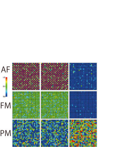
$\rho_{a}$              $\rho_{b}$                 $\rho_{h}$

Figure 5: Snapshots of three densities $\rho_{a}$, $\rho_{b}$, and $\rho_{h}$ of Eq.(3.4) in a XY plane in three phases of Fig.1 for $L=24$. From the above, $(c_{1},\alpha)=(3.0,-0.5)$ (AF phase), $(c_{1},\alpha)=(3.0,-1.5)$ (FM phase), and $(c_{1},\alpha)=(0.5,-0.5)$ (PM phase).

III.2 Superfluid

In this subsection, we shall consider the case of finite hopping amplitude $t$. We verified numerically that the global phase structure of Fig.1 remains intact for small $t$ (i.e., $c_{3}$). However as $c_{3}$ is increased, phase transition to SF state takes place at some critical values $c_{3}=c_{3c}(c_{1},\alpha)$. The transition from the AF phase at $c_{3}<c_{3c}$ to the SF phase at $c_{3}>c_{3c}$ is of strong first order as $U$ and the hole density $\rho_{h}$ in Fig.6 show. We employed the specific update methods for the MC simulations in order to generate pre-choice configurations efficiently for the first-order phase transitionBtJ1 ; nakano . Nevertheless, the obtained $U$ and the hole density $\rho_{h}$ exhibit large hysteresis loops as $c_{3}$ varies.

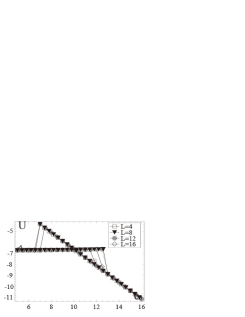
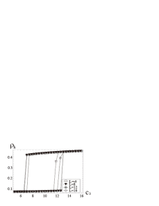
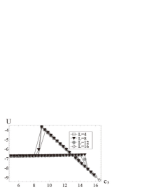
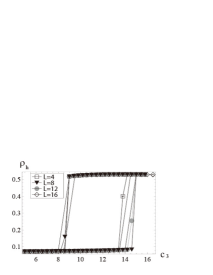
Figure 6: $U$ and the hole density $\rho_{h}$ as a function of $c_{3}$ for $\alpha=-0.5$ (upper panels) and $0.5$ (lower panels) with $c_{1}=3.0$. Hysteresis loop indicates the transition from AF state to SF is of first-order. Similar hysteresis loops are obtained for other values of $\alpha$ and $c_{1}$ for the AF phase.

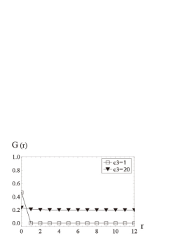
Figure 7: Boson correlation function $G(r)=G_{a}(r)=G_{b}(r)$ for $c_{1}=3.0$, $\alpha=0.5$. Finite LRO for $c_{3}=20$ indicates that the phase transition in Fig.6 is a SF transition.

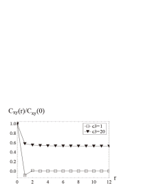
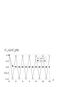
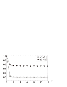
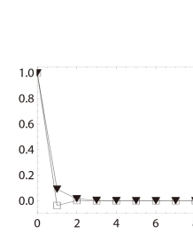
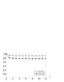
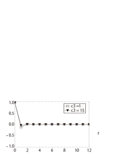
Figure 8: (Top) Pseudo-spin correlation functions $C_{xy}(r)$ and $C_{z}(r)$ in the AF and SF states for $\alpha=0.5$ and $c_{1}=3.0$. In SF state, a FM LRO appears in the $xy$-plane of the pseudo-spin space. (Middle) $C_{xy}(r)$ and $C_{z}(r)$ in the PM and SF states for $\alpha=-1.5$ and $c_{1}=0.5$. (Bottom) $C_{xy}(r)$ and $C_{z}(r)$ in the FM and SF states for $\alpha=-1.5$ and $c_{1}=3.0$.

To verify that the SF state is realized for $c_{3}>c_{3c}$, we calculated the boson correlation function $G_{a}(r)$ and $G_{b}(r)$,

$$G_{a}(r) = {1\over L^{3}}\sum_{r_{0}}\langle\phi^{\dagger}_{r_{0}}z_{1,r_{0}}z^{\dagger}_{1,r_{0}+r}\phi_{r_{0}+r}\rangle,$$

$$G_{b}(r) = {1\over L^{3}}\sum_{r_{0}}\langle\phi^{\dagger}_{r_{0}}z_{2,r_{0}}z^{\dagger}_{2,r_{0}+r}\phi_{r_{0}+r}\rangle,$$ (3.5)

and if $G_{a}(r),\;G_{b}(r)\rightarrow$ finite as $r\rightarrow\infty$, the SF is realized. The results are shown in Fig.7. It is obvious that $G_{a}(r)=G_{b}(r)$ in the present case, and it has a nonvanishing LRO for $c_{3}=20$ indicating existence of a finite density of SF. In Fig.8 we also show the calculation of the pseudo-spin correlation functions $C_{z}(r)$ and $C_{xy}(r)$. The results show that the phase transition to the SF state accompanies a transition from the Ising-like AF LRO to the XY-FM LROFMSF . This result is in sharp contrast with the result obtained by the MFT. The present numerical study indicates that the SS phase predicted in MFT, in which the AF LRO and SF coexist, does not appear in the present model. As the phase transition to the SF phase takes place at $c_{3}=\beta t\sim O(10)$ and $c_{1}[\sim O({\beta t^{2}\over U},{\beta t^{2}\over V})]=3$, the critical region is located at $t/U,\ t/V\sim 3/10\ll 1$ in the original Hubbard model. Therefore the above obtained results in the $t$-$J$ model are also applicable for the bosonic Hubbard model.

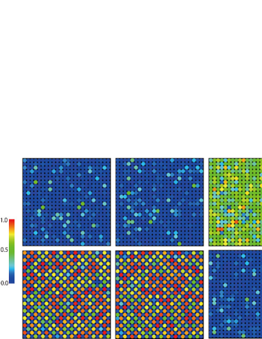
$\hskip 28.45274pt\rho_{a}$               $\rho_{b}$                 $\rho_{h}$

Figure 9: Snapshots of three densities $\rho_{a}$, $\rho_{b}$, and $\rho_{h}$ of Eq.(3.4) in a XY plane for $L=24,c_{1}=3.0,c_{3}=10.0,\mu=0.0,\alpha=0.5$. The upper ones are in the FM+SF phase with the higher energy $U/N=-4.39$ and the lower ones are in the AF phase with the lower energy $U/N=-6.68$.

There are two kinds of SF, one made of atom $a_{r}$ and the other made of $b_{r}$. It is interesting to see how each SF behaves in the hysteresis region of the first-order phase transition. In Fig.9 we present snapshots of typical configurations of $\rho_{a}$ and $\rho_{b}$ for $c_{3}=10.0$ to check the possibility that the AF solid and SF exist separately in every state of update. We found that on the $c_{3}$-decreasing line of the hysteresis loop the pure FM+SF state is realized, whereas the pure AF state exists on the $c_{3}$-increasing line. This indicates that in real experiments there exists a genuine phase transition point in the middle of the hysteresis loop in the MC simulation and the internal energy has a sharp discontinuity at that transition point. At the discontinuity point, immiscible state of the AF solid and SF is realized. In order to verify this expectation, we performed MC simulation starting with a half-AF and half-SF configuration and searched a “genuine critical coupling” $c_{3c}$ at which this phase-separated configuration is stable during MC update. For $\alpha=0.5$ and $c_{1}=3.0$, we found $c_{3c}=11.36$, see Fig.10. This result, which shows that the phase separation takes place in the present 3D system, is consistent with the result of the previous study on the system at $T=0$BtJ2 .

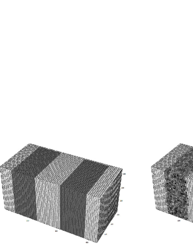
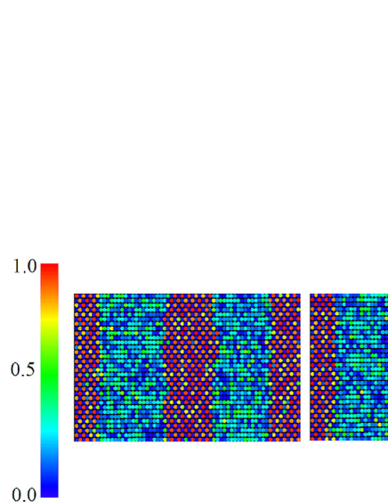
$\hskip 28.45274pt\rho_{a}$               $\rho_{b}$                 $\rho_{h}$

Figure 10: (Upper panels) (Left) Initial configuration with phase separation and (Right) configuration after $60\times 10^{5}$ sweeps at the critical point. Dark regions represent SF with relatively high hole density and bright regions represent AF solid. (Lower panels) Densities $\rho_{a}$, $\rho_{b}$ and $\rho_{h}$ in a horizontal plane in configuration after $60\times 10^{5}$ sweeps.

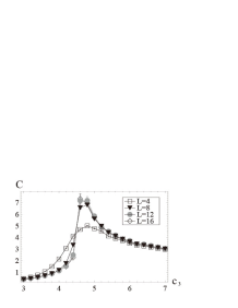
Figure 11: Transition from PM to FM+SC. Specific heat for $c_{1}=0.5$ and $\alpha=-1.5$ vs $c_{3}$. The peak of $C$ has a systematic $L$ dependence of a typical second-order transition.

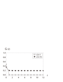
(a)                                (b)

Figure 12: Boson correlation function $G(r)=G_{a}(r)=G_{b}(r)$ for $c_{1}=0.5$, $\alpha=-1.5$ (Left) and $c_{1}=3$, $\alpha=-1.5$ (Right). Finite LRO for $c_{3}=15$ indicates that the phase transition in Figs.11 and 13 is a SF transition.

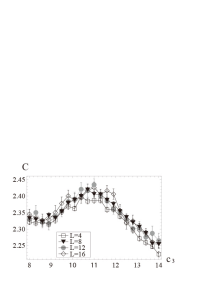
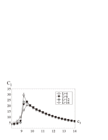
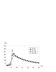
Figure 13: Specific heat of phase transition from FM to FM+SC, $c_{1}=3.0$ and $\alpha=-1.5$ exhibits rather peculiar behavior, whereas specific heat of each term $c_{1}$, $c_{3}$ shows typical system-size dependence of second-order phase transition.

Let us turn to the PM $\rightarrow$ SF transition. In Fig.11 we present $C$ for $c_{1}=0.5$ and $\alpha=-1.5$. $C$ exhibits a sharp peak at $c_{3}\simeq 4.6$, which indicates existence of a second-order phase transition. We calculated the boson correlation function and verified that a SF appears for $c_{3}>4.6$. See Fig.12a.

We also verified that a transition from the FM to FM+SC takes place as $c_{3}$ is increased. In the critical region, the total specific heat $C$ exhibits rather peculiar behavior, but the “specific heat” of each term, defined by $c_{i}\equiv\langle(E_{i}-\langle E_{i}\rangle)^{2}\rangle/L^{3}$ for each term $E_{i}$ in the Hamiltonian, shown in Fig.13 exhibits typical behavior of the second-order phase transition. In Fig.12b, we show the boson correlation function for Fig.13. The existence of the finite LRO means that the phase transition in Fig.13 is again a transition to SF.

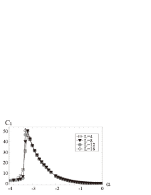
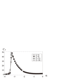
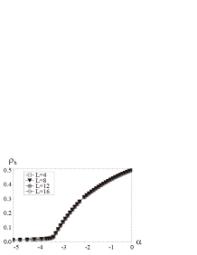
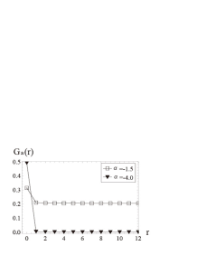
Figure 14: Specific heat of each term as a function of $\alpha$ for $c_{1}=3.0$ and $c_{3}=20$. There exist no anomalous behavior at $\alpha\simeq-1$. Peaks in the specific heats at $\alpha\simeq-3.2$ mean a phase transition to vanishing SF, for hole density is vanishingly small and boson correlation vanishes for $\alpha<-3.2$.

We observed that all three phases at $t=0$, i.e., PM, AF and FM phases, evolve into the SF state as $t$ is increased. Then, it is quite interesting to see if there is a phase boundary between these SF’s for sufficiently large $c_{3}$ though all of three phases belong to the FM$+$SF phase. This problem is closely related with recent experiment investigating two species SF2BEC . This experiment observed that (im)miscibility of two SF’s depends on the inter and intra-interactions between atoms. In Fig.14, we show the specific heat of each term and particle density as a function of $\alpha$ for $c_{1}=3.0$ and $c_{3}=20$. On may expect that there is a phase boundary separating two FM$+$SF phases at $\alpha\simeq-1$, but the result exhibits no anomalous behaviors there. On the other hand, the peaks at $\alpha\simeq-3.2$ accompanies abrupt decrease of the hole density. This indicates that there exists a phase transition and that is a transition into the vanishing SF. $G_{a}(r)$ and $G_{b}(r)$ in Fig.14 support this interpretation because they have no RLO at $\alpha=-4.0$. The phase $\alpha<-3.2$ is a pure FM state without holes. We also studied whether phase transition between two SF’s takes place as the value of $c_{1}$ is varied, but we found a similar result to the above as varying $\alpha$, i.e., there exists no phase transition between two SF’s.

IV Conclusion

In present paper, we studied the $t$-$J$ model of two-component hard-core bosons by means of MC simulations. We considered the system with filling factor up to unity, and obtained the global phase diagram in the grand-canonical ensemble (GCE). At vanishing hopping amplitude, there are three phases in the $\alpha-c_{1}$ plane, PM, AF and FM phases. As the hopping amplitude is increased, all three phases evolve into SF state with BEC of atoms. These obtained results are globally consistent with those for the case of integer fillings obtained by MFT-type approximation and numerical methodsaltman ; soyler . However, we verified that the SS state, which is predicted to appear by the MFT, does not exist in the present model in the GCE. On the other hand, we found that the phase separation of the AF solid and SF is realized at the phase transition point.

We also studied if there exists phase boundary between the SF’s. However there are no phase boundaries between them.

Results obtained in the present paper show that the bosonic $t$-$J$ model has a very rich phase structure. We studied the system in the GCE. It is quite interesting to study the bosonic $t$-$J$ model in the canonical ensemble with fixed average atomic number. In particular, an inhomogeneous state may appear near the first-order phase transition point from the AF solid to the SF. This problem is under study and results will be reported in a future publication.