3D simulations of pillars formation around HII regions: the importance of shock curvature

Abstract

Aims. Radiative feedback from massive stars is a key process to understand how HII regions may enhance or inhibit star formation in pillars and globules at the interface with molecular clouds. We aim to contribute to model the interactions between ionization and gas clouds to better understand the processes at work. We study in detail the impact of modulations on the cloud-HII region interface and density modulations inside the cloud.

Methods. We run three-dimensional hydrodynamical simulations based on Euler equations coupled with gravity using the HERACLES code. We implement a method to solve ionization/recombination equations and we take into account typical heating and cooling processes at work in the interstellar medium and due to ionization/recombination physics.

Results. UV radiation creates a dense shell compressed between an ionization front and a shock ahead. Interface modulations produce a curved shock that collapses on itself leading to stable growing pillar-like structures. The narrower the initial interface modulation, the longer the resulting pillar. We interpret pillars resulting from density modulations in terms of the ability of these density modulations to curve the shock ahead the ionization front.

Conclusions. The shock curvature is a key process to understand the formation of structures at the edge of HII regions. Interface and density modulations at the edge of the cloud have a direct impact on the morphology of the dense shell during its formation. Deeper in the cloud, structures have less influence due to the high densities reached by the shell during its expansion.

1 Introduction

Radiative feedback from massive stars might be an important process to explain the star formation rates on galactic scales. Its role in complexe structures like giant molecular clouds is still a matter of debate (see Dale et al., 2007; Price et al., 2010; Dale & Bonnell, 2011). When the UV radiation from the massive objects photoionize the surrounding gas, a ”bubble” of hot ionized gas expands around the star: the HII region (see Purcell et al., 2009, for example). While star formation is inhibited inside the bubble, the small-scale compression at the edge of the HII region, due to its expansion, seems to form elongated structures (pillars) and globules in which the star formation activity seems enhanced (see Deharveng et al., 2010, for example). Different models investigate this process.
First studies of HII regions (e.g. Strömgren, 1939; Elmegreen & Lada, 1977) show how UV radiation leads to the formation of an ionization front and of a shock ahead. The gas is compressed between them, forming a dense shell which may lead to fragmentation, gravitational collapse and star formation, this is the collect and collapse scenario (Elmegreen & Lada, 1977).
An other one was proposed by Bertoldi (1989), the radiation-driven implosion scenario. He looks at the photoevaporation of spherical neutral clouds and finds that the ionization front drives a shock into the cloud leading to the compression of the initial structure into a compact globule. This scenario has been studied in detail with numerical simulations for years (see Lefloch, B. & Lazareff, 1994; Williams et al., 2001; Kessel-Deynet & Burkert, 2003). Recently, Bisbas et al. (2009) and Gritschneder et al. (2009) looked at the implosion of isothermal spherical clouds with smoothed particle hydrodynamics (SPH) codes. Using a grid code, Mackey & Lim (2010) produce elongated structures from dense spherical clumps using the shadowing effects of these structures.
In the last decade, the importance of the initial turbulence in the cloud has been studied with three-dimensional simulations, at different scales. Mellema et al. (2006) present simulations of the formation of the HII region with a good agreement with observations. The interplay between ionization and magnetic fields has been studied by Krumholz et al. (2007) and later by Arthur et al. (2011), in the context of HII region formation, finding that magnetic fields tend to suppress the small-scale fragmentation. On larger scales Dale et al. (2007) look at the impact of ionization feedback on the collapse of molecular clouds finding a slight enhancement of star formation with ionization while Dale & Bonnell (2011) finds almost no impact. On smaller scale, Lora et al. (2009) find that the angular momentum of the resulting clumps is preferentially oriented perpendicular to the incident radiation. Gritschneder et al. (2010) show that pillars arise preferentially at high turbulence and that the line-of-sight velocity structure of these pillars differs from a radiation driven implosion scenario.

These HII regions are seen in a lot of massive molecular clouds and are the object of a large number of observation- nal studies: in Rosette nebula (Schneider et al., 2010), M16 (Andersen et al., 2004), 30 Doradus (Walborn et al., 2002), Carina nebula (Smith et al., 2000), Elephant Trunk nebula (Reach et al., 2004), Trifid nebula (Lefloch et al., 2002), M17 (Jiang et al., 2002) or also the Horsehead nebula (Bowler et al., 2009). Spitzer observations provide also a wide range of HII regions studied in detail by Deharveng et al. (2010). Pillars and globules are often seen and present density clumps which may lead to star formation. The different scenarii described above can be constrained thanks to these observations.

The present study focuses on ”simple” situations in order to highlight the key mechanisms at work in the interaction between a HII region and a cloud. We present the numerical methods needed for this study and then two different set ups, cloud-HII region interface modulation and density modulation inside the cloud and finally a study of the different stage of evolution of the resulting pillars. A following paper will investigate these situations in a more complete set up which will include turbulence inside the cloud.

2 Numerical methods

We consider a molecular cloud impacted by the UV radiation of a OB cluster to study how structures develop at the interface between the resulting HII region and the cloud. Subsection 2.1 describes the method used to simulate gas hydrodynamic in the molecular cloud with the HERACLES code (González et al., 2007). Subsection 2.2 describes the numerical method used to take in account the UV radiation from the OB cluster and the resulting ionization/recombination reactions. Thermal processes from these reactions and the heating and cooling rates used in the molecular cloud are described in subsect. 2.3.

2.1 Hydrodynamic

Our simulations are performed with the HERACLES code. It is a grid-based code using a second order Godunov scheme to solve Euler equations. These equations are given in Eq. 1 in a presence of a gravitationnal potential $\Phi$, constrained by the Poisson equation: $\triangle\Phi=4\pi G\rho$.

$$\frac{\partial\rho}{\partial t}+\nabla\cdot(\rho\textbf{V}) = 0\quad,$$ (1)

$$\frac{\partial\rho\textbf{V}}{\partial t}+\nabla\cdot[\rho\textbf{V}\otimes\textbf{V}+pI] = -\rho\nabla\Phi\quad,$$ (2)

$$\frac{\partial E}{\partial t}+\nabla\cdot[(E+p)\textbf{V}] = -\rho(\textbf{V}\cdot\nabla\Phi)+\Lambda(\rho,T)\quad.$$ (3)

We use an ideal gas equation of state, so that $E=p/(\gamma-1)+0.5\rho\textbf{V}^{2}$ with $\gamma=5/3$. $\Lambda(\rho,T)$ corresponds to the heating and cooling processes detailed in subsect. 2.3 leading to a polytropic gas of index around 0.7 at equilibrium (for $\rho=500/cm^{3}$). All the other variables have their usual meaning.

2.2 Ionization

The stationnary equation governing radiative tranfer in spherical geometry is given by:

$$\mu\partial I_{\nu}/\partial r+(1-\mu^{2})/r\times\partial I_{\nu}/\partial\mu=-\kappa_{\nu}I_{\nu}+\eta_{\nu}$$ (4)

$\mu$ is equal to $\cos\theta$ and $\theta$ is the polar angle, $I_{\nu}(r,\mu,\nu)$ is the spectral intensity at a radius r in the direction defined by $\mu$ at the frequency $\nu$, $\kappa_{\nu}(r,\nu)$ is the absorption coefficient and $\eta_{\nu}(r,\nu)$ is the source term. Radiation is coming from a point source such that $I_{\nu}(r,\mu,\nu)=F_{\nu}(r,\nu)\times\delta_{1}(\mu)$, in which $\delta_{1}(\mu)$ is a Dirac distribution whose peak is at $\mu=1$ corresponding to the direction $\theta=0$ in spherical coordinates. Integrating Eq. 4 over $\mu$ leads to Eq. 5 in which the absorption coefficient and the source term are given by Eq. 6.

$$\partial F_{\nu}/\partial r+2/r\times F_{\nu}=-\kappa_{\nu}F_{\nu}+\eta_{\nu}$$ (5)

$$\eta_{\nu}(r,\nu) = S_{*}(\nu)\delta_{0}(r)$$ (6)

$$\kappa_{\nu}(r,\nu) = \sigma n_{H_{0}}\nu^{3}_{1}/\nu^{3}$$ (7)

$h\nu_{1}$ is equal to 13.6eV, $\sigma$ is the ionizing cross section for photons at frequency $\nu_{1}$ and $n_{H_{0}}(x)$ the density of neutral hydrogen atoms. $\delta_{0}(r)$ is a Dirac peak at r=0 and $S_{*}$ is the flux from the central OB cluster. The radiation from the cluster is approximated by an unique source of radius $r_{*}$ at a distance $r_{0}$ of the computational domain, $S_{*}$ corresponds to a diluted planckian function at the star temperature: $S_{*}(\nu)=\pi(r_{*}^{2}/r_{0}^{2})B_{\nu}(T_{*})$. By dividing Eq. 5 with $h\nu$ to have an equation on the number of photons rather than radiative energies and averaging $\nu$ between $\nu_{1}$ and $+\infty$ in order to keep track only of the ionizing photons, we get:

$$1/r^{2}\times d(r^{2}F_{\gamma})/dr=-n_{H_{0}}\bar{\sigma}_{\gamma}F_{\gamma}+\delta_{0}(r)\bar{S}_{*}$$ (8)

$F_{\gamma}$ is now the number of ionizing photons per unit of surface and time arriving in the radial direction and $\bar{\sigma}_{\gamma}$ is the average cross-section over the planckian source at $T_{*}$ and $\bar{S}_{*}$ the rate of emission of ionizing photons by the stars. We can get plane-parallel equations in the limit $r\rightarrow\infty$.

We now compute the equations for photo-chemistry. We set $X$ to be the fraction of ionization $X=n_{H^{+}}/n_{H}$ in which $n_{H}=n_{H^{+}}+n_{H^{0}}$, it follows the dynamic of the gas as an advected quantity. The variation of protons is the number of incoming photons which are going to interact minus the number of protons which will be used for recombination. The number of interacting photons in a volume $dv_{cell}$ is given by the number of incoming photons threw a surface $ds_{in}$ multiplied by the probability of interaction given by the cross-section, $dP=\bar{\sigma}_{\gamma}n_{H^{0}}dr$ leading to:

$${d(Xn_{H})} = dn_{\gamma_{int}}-dn_{H_{rec}}$$ (9)

$$dn_{H_{rec}} = \beta n_{H^{+}}n_{e^{-}}dt=\beta X^{2}n_{H}^{2}dt$$ (10)

$$dn_{\gamma_{int}} = F_{\gamma}(r)ds_{in}dtdP/dv_{cell}=\bar{\sigma}_{\gamma}F_{\gamma}n_{H}(1-X)\omega dt$$ (11)

The dilution term $\omega=(ds_{in}dr/dv_{cell})$ is equal to $r_{in}^{2}/r_{cell}^{2}$ in spherical coordinates and to 1 in the plan-parallel limit. $r_{in}$ is the radial position of the entrance surface for incoming photons $ds_{in}$ and $r_{cell}$ is the radial position of the centre of the volume $dv_{cell}$. $\beta$ gives the rate of recombination and is equal to $2\times 10^{-10}T^{-0.75}$ $cm^{3}/s$ in which $T$ is the temperature of thermodynamic equilibrium between all the species (see Black, 1981).

2.3 Thermal processes

Thermal processes are taken in account by adding the heating and cooling rate $\Lambda(\rho,T)$ in the equation of energy conservation in Eq. 1.

In the ionized phase, we consider two processes which have a major impact on the thermodynamic of the gas, the photoelectric heating due to the massive stars UV flux and the cooling due to recombination of electrons onto protons. The energy $e_{\gamma}(T_{*})$ given by ionizing photons is the integrated value of $I_{\nu}/h\nu(h\nu-h\nu_{1})$ between $\nu_{1}$ and $+\infty$ on the incoming spectrum $I_{\nu}$. In the following we will assume a planckian distribution $B_{\nu}(T_{*})$ with $T_{*}=35OOOK$ which gives $e_{\gamma}(T_{*})=1eV$. Therefore the heating rate is given by Eq. 12. The cooling term is the loss of the thermal energy of electrons used by recombination given by Eq. 13.

$$\mathcal{H}=dn_{\gamma_{int}}/dt\times e_{\gamma}=\omega(1-X)n_{H}F_{\gamma}\bar{\sigma}_{\gamma}e_{\gamma}$$ (12)

$$\mathcal{L}=dn_{H_{rec}}/dt\times k_{b}T/(\gamma-1)=\beta X^{2}n_{H}^{2}k_{b}T/(\gamma-1)$$ (13)

At the equilibrium between ionization and recombination, the recombination rate is equal to the ionization rate $dn_{\gamma_{int}}=dn_{H_{rec}}$. Therefore when thermodynamic equilibrium is achieved in the ionized phase the temperature is given by $(\gamma-1)e_{\gamma}/k_{b}$ which is equal to 7736 Kelvin. The corresponding isothermal curve in the pressure-density plane is drawn in Fig. 1.

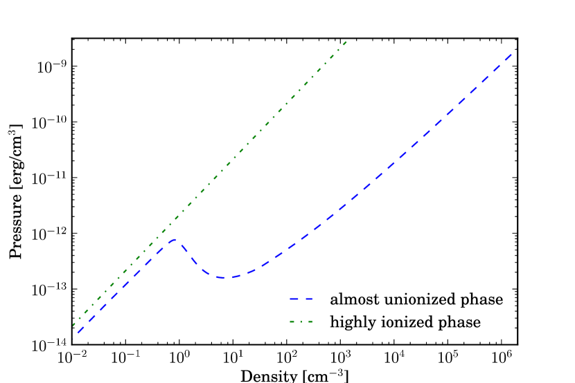
Figure 1: Thermodynamic equilibrium in the pressure-density plane for the highly and weakly ionized phases

In the weakly ionized phase, we simulate the radiative heating and cooling of the interstellar medium (ISM) by adding five major processes following the work of Audit & Hennebelle (2005) and Wolfire et al. (1995, 2003):

• Photoelectric heating by UV radiation with a flux equal to $G_{0}/1.7$ in which $G_{0}$ is the Habing’s flux

• cooling by atomic fine-structure lines of CII

• cooling by atomic fine-structure lines of OI

• cooling by H (Ly$\alpha$)

• cooling by electron recombination onto positively charged grains

The UV flux used in this phase is an ambiant low flux, additional to the UV flux $F_{\gamma}$ coming from the massive stars, which is used in our ionization process described in subsect. 2.2. This heating and cooling function is only valid for the dense cold and weakly ionized phase. Therefore these processes are weighted by $1-X$ and contribute only in the weakly ionized phase. In this phase, the ionization fraction used for the thermal processes is a function of the temperature and is given by Wolfire et al. (2003) (typically around 10^-4). The thermodynamic equilibrium in the pressure-density plane is given in fig. 1.

The transition at the ionization front is very sharp as it can be seen on the tests in subsect. 2.4. Therefore the fraction of the gas in between the two phases is small and is not dynamically significant.

2.4 1D spherical test: HII region expansion in spherical geometry

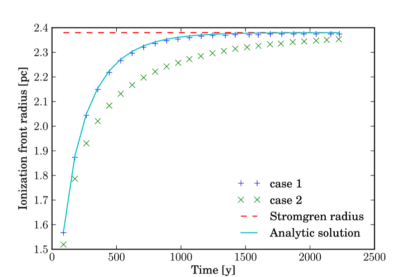
Figure 2: Expansion of an HII region in a homogenous medium (n_H=500 cm^-3, T$\approx$25 K, S_∗=10⁵⁰ $\gamma_{ionizing}$/s). Case 1 is a simulation in which the gas temperature is instantaneously put at 7736 K when the ionization fraction is bigger than 0.5. Case 2 takes into account the time evolution of temperature given by Eq. 12 and 13. The analytic solution is computed from Eq. 15 when the thermal equilibrium is reached instantaneously. The Strömgren radius is given by Eq. 14.

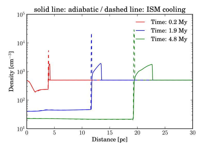
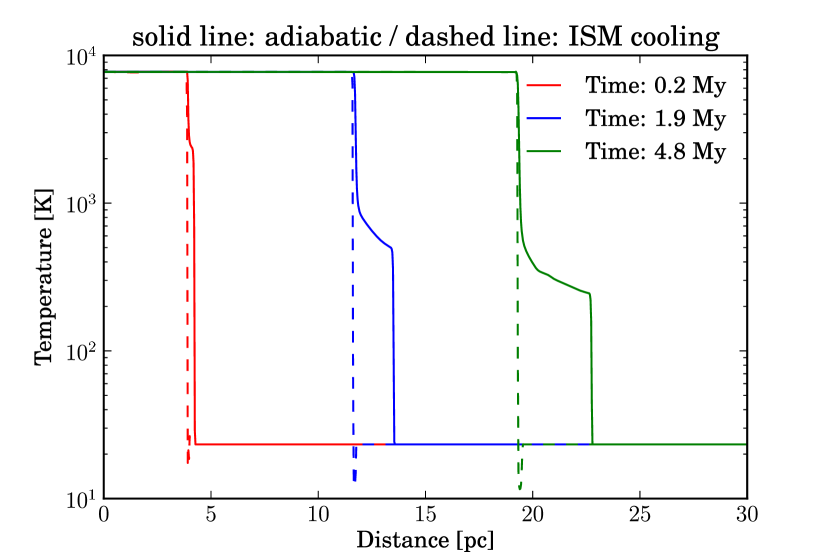
Figure 3: Density (top) and temperature (bottom) profiles of the expansion of an HII region in a homogenous medium (n_H=500 cm^-3, T$\approx$25 K, S_∗=10⁵⁰ $\gamma_{ionizing}$/s). Solid lines correspond to an adiabatic cold phase and dashed lines to a cooled cold phase with the cooling described in Subsect. 2.3

We first start by testing our numerical algorithms on a simple 1D spherical test which can be compared to analytical solution. Starting from a region with n_H = 500 cm^-3 and T $\approx$ 25 K, we switch on a photon flux coming from a typically O4 star with $\bar{S}_{*}$ = 10⁵⁰ $\gamma_{ionizing}/s$. At the beginning the typical time for ionization/recombination is much shorter than the hydrodynamical typical timescale. Therefore there is a first phase of development in which the hydrodynamic is frozen and the medium is ionized in a small sphere around the source. The radius of this sphere is controlled by the Strömgren formula given in Eq. 14 (see Strömgren, 1939). Ionization stops when all photons are used to compensate recombinations inside the sphere. In our example this radius is R_s = 2.38 pc.

$$R_{s}=\left(\frac{3S_{*}}{4\pi\beta n_{H}}\right)^{1/3}$$ (14)

If the thermal equilibrium between ionization and recombination is reached instantaneously, it is possible to compute an analytic expression of the time evolution of the ionization front (Spitzer, 1978):

$$R_{i}=R_{s}(1-e^{-\beta n_{H}t})^{1/3}$$ (15)

The development of the ionized sphere before hydrodynamic starts to matter is shown in Fig. 2. Two cases are treated numerically, first the thermal equilibrium is reached instantaneously and the gas temperature is switched at 7736 K when the ionization fraction is bigger than 0.5. It allows us to compare our numerical solution to the analytic formula given in Eq. 15: the error is less than 0.5%. Second we resolve numerically the time evolution of the temperature given by the balance between Eq. 12 and 13. The ionization front is slowed down by the explicit treatement of cooling due to recombination. The recombination rate increases when the temperature decreases leading to a lower penetration of ionizing photons.

After this first step the energy deposited by the ionizing photons creates a spherical region with a high pressure. This region will therefore start expanding and pushing the surrounding interstellar matter, creating a shock front ahead the ionization front. This process creates an expanding ionized cavity and a shell of compressed gas. Typical density and temperature profiles are given in Fig. 3. Solid lines corresponds to the adiabatic case for the cold gas and the dashed lines to the cooling function described in Subsect. 2.3. The shock front is cooled down by the thermal processes and the shell is compressed up to two order of magnitude. This phenomenon is at the origin of the idea of the collect and collapse scenario for triggered star formation around HII regions proposed by Elmegreen & Lada (1977).

We can derive the equations governing the density, the speed and the thickness of the shell in the approximation of an isothermal D-critical shock following Elmegreen & Lada (1977); Spitzer (1978). The density and the pressure when the HII region has a radius r can be derived from the equilibrium between ionization and recombination in the sphere and are given by:

$$n_{II} = n_{0}(r_{s}/r)^{\alpha}$$ (16)

$$p_{II} = 2n_{II}k_{b}T_{II}$$ (17)

$\alpha$ is equal to 1/3 and $r_{s}$ to $(3S_{*}/4\pi n_{0}^{2}\beta)^{1/3}$ in spherical geometry while, in the plan-parallel limit, $\alpha$ is equal to 1/2 and $r_{s}$ to $F_{\gamma}/n_{0}^{2}\beta$. The parameters of the shell can be computed using Eq. 16 and assuming a shell temperature $T_{shell}$ and the corresponding sound speed $c_{shell}$ (for details, see Elmegreen & Lada, 1977). They are given by Eq. 18 in which $n_{shell}$ is the maximum density in the shell, $v_{shell}$ the shock speed, and $l_{shell}$ the typical width of the shell.

$$n_{shell} = \gamma p_{II}/c_{shell}^{2}/(\mu m_{H})$$ (18)

$$v_{shell} = (8p_{II}/3\rho_{0})^{1/2}$$ (19)

$$l_{shell} = 4r/\gamma c_{shell}^{2}/v_{shell}^{2}$$ (20)

Assuming a temperature in the shell of 10 kelvin and a radius of 20 parsecs for the HII region we get a shell density of 3.2$\times$10⁴cm^-3, a speed of 3.2 km/s and a width of 0.5 parsec. These values are in good agreement with the shell parameters we obtain in the 1D simulation in Fig. 3, the maximum density when the HII-region radius is 20 parsecs is 2.9$\times$10⁴cm^-3, the shell speed 4.4 km/s and the shell width 0.27 parsec. We can see that our code can follow with very good accuracy the ionization front and the subsequent evolution of the dense shell. We will therefore now turn our attention to more interesting 3D cases.

3 Forming pillars

The interstellar medium has a very complex structure with important inhomogeneities and large density fluctuations. The passage from 1D to 3D brings a lot of new degrees of freedom. It allows us to study how the shell resulting from the collect and collapse scenario may be perturbed. The possibility to have localized density gradients has been extensively studied with the radiation driven implosion scenario (Mackey & Lim, 2010; Bisbas et al., 2009; Gritschneder et al., 2009) and more recently within a turbulent media (Gritschneder et al., 2010). In this work, we first want to focus on more simple and schematic situations in which the physical processes at work can be identified and studied more easily. We will therefore study two idealized cases. First we will look at the interaction of the ionization front with a medium of constant density having a modulated interface. Then we will consider a flat interface but the presence of overdense clumps in the medium.

3.1 From interface modulations to pillars

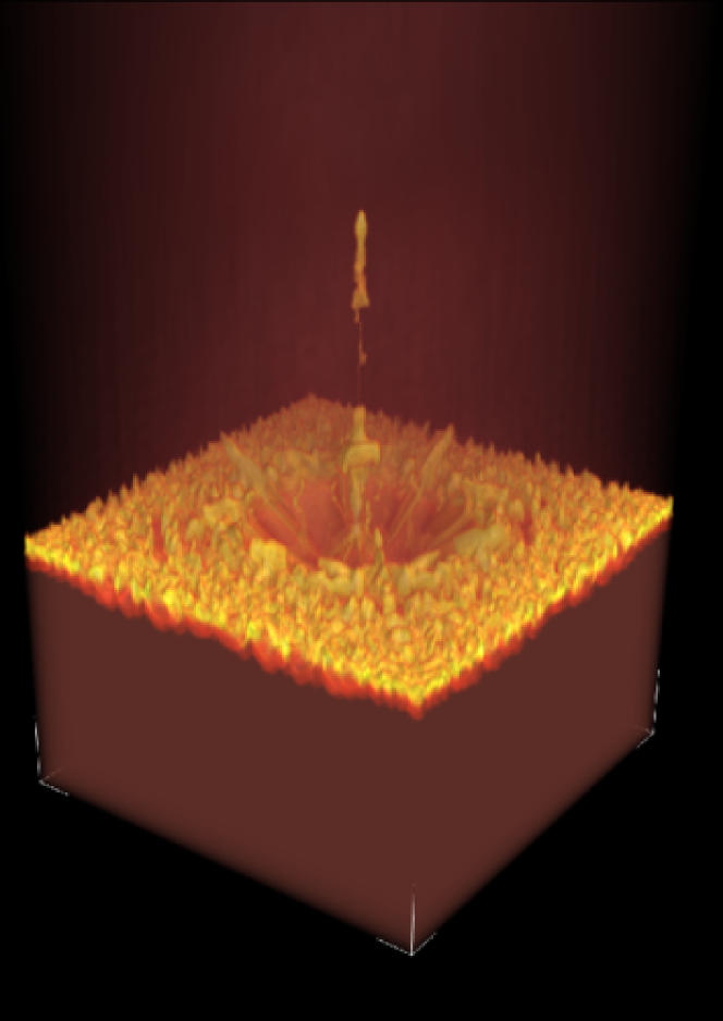
Figure 4: 3d snapshot of density at 500 ky of an ionization front propagation with a modulated interface. The UV flux at the top of the box is 10⁹ photons per second per square centimetre, the box is 4x2x2 parsecs. The dense gas is initially at 500 H/cm³ at a temperature around 25 K (thermal equilibrium from Fig. 1). The (base width)/height ratios (w/h ratios hereafter) of the modulation is w/h=0.9.

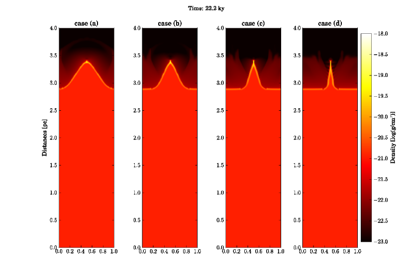
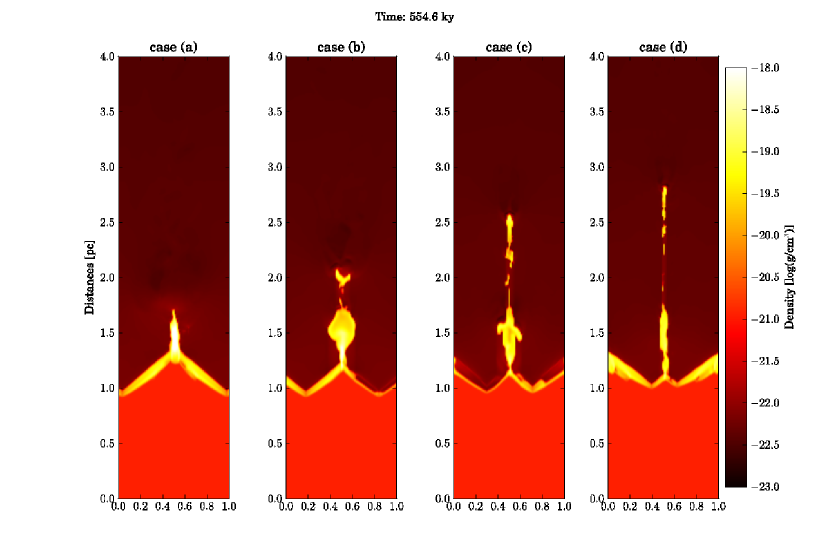
Figure 5: Density cuts of four simulations of an ionization front propagation with a modulated interface. The UV flux at the top of the box is 10⁹ photons per second per square centimetre, the box is 4x2x2 parsecs (half of the cut is shown). The dense gas is initially at 500 H/cm³ at a temperature around 25 K (thermal equilibrium from Fig. 1). The (base width)/height ratios of the modulations are respectively 2 for case (a), 1.4 for case (b), 0.9 for case (c) and 0.5 for case (d).

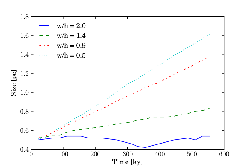
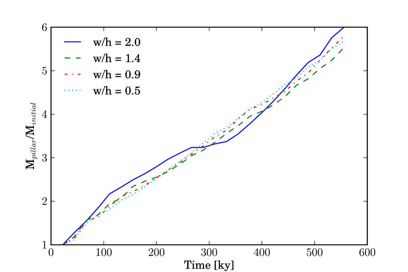
Figure 6: Monitoring of the size (top) and the mass (bottom) of pillars identified in Fig. 5. The size is calculated by the difference of the average position of the ionisation front and the its position at the centre of the y-z plane (head of the initial structure). The mass is calculated in a box between the two vertical positions defined to calculated the size and with a width defined by the width of the initial structure and is normalized by the mass in the initial modulation.

We first study the interaction between the ionization front and an interface modulated by an axisymmetric sinus mode with constant heigh (amplitude of 0.5 parsec) and four different base widths (see Fig. 4 and Fig. 5). The size of the computational domain is adapted to the typical observed length scale of pillars, $4\times 2\times 2$ pc³, at a resolution of $400\times 200\times 200$ corresponding to spatial resolution of $1\times 10^{-2}$ pc. The boundary conditions are periodic in the directions perpendicular to the ionization propagation direction, imposed where the flux is incoming and free flow at the opposite. Ionization processes introduced in subsect. 2.2 are taken in the plan-parallel limit. The snapshots around 500 ky show that the narrower the initial structures, the longer the resulting pillars. With a (base width)/heigh ratio (w/h ratio hereafter) of 0.5 we get a structure whose size was almost multiplied by 3.5 in 500 ky. Besides the initial structures have less and less mass with decreasing widths and still manage to form longer pillars as can be seen on figure (5). High densities or high initial mass are not needed to form structures which are going to resist the ionization. The important factor here is how matter is distributed in space and interact with the propagating shock. Very little and low-density material well distributed in space can result in a long pillar-like structure. We will call these structures pillars hereafter, however a detailed comparison with observations is needed to see whether these structures emerging from idealized scenarii are a good approximation of the reality or not.

To study the properties of the pillars, we monitor their sizes and masses in Fig. 6. The size gain identified previously is a continuous process in time at an almost constant speed which depends very strongly on the width/heigh ratio. Narrow initial modulation have a very fast growth while larger one grow slowly, if at all. The mass increase relative to the initial mass of the structure is almost the same in all simulations and does not seems to depend on the initial w/h ratio. It reaches a factor of 5-6 in 500 ky.

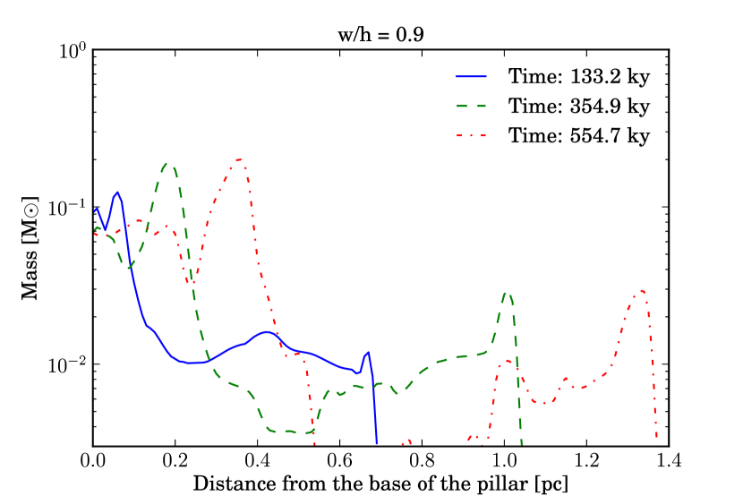
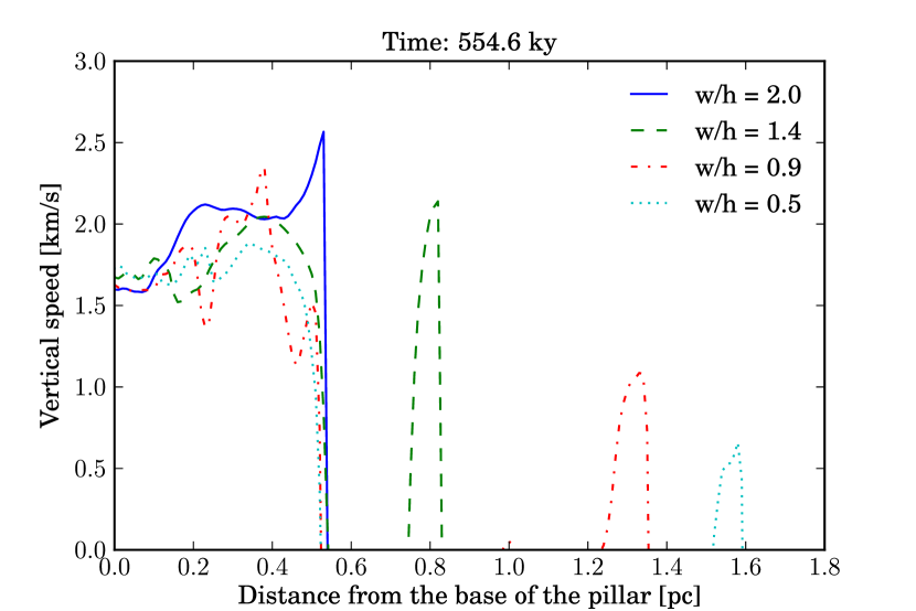
Figure 7: Mass profiles (top) and vertical velocity profiles (bottom) at three different times of the pillar in the w/h = 0.9 simulation. These profiles are made within the boxes defined in Fig. 6

.

Vertical profiles of the mass in the pillars (see Fig. 7) show that the mass gain identified in Fig. 6 is accumulated at the base. The mass of the head of the pillar slightly increases and then remains stable during the simulation while the central part connecting the head and the base is stretched and its mass decreases. The profiles of the vertical speed show that the bases of the pillars have a roughly constant speed and the size variations are due to vertical speed difference of the heads. The differences between the sizes of the pillars can be directly deduced from the velocity differences of the heads: a velocity difference of 0.5 km/s during 500 ky gives a spatial difference of 0.25 pc which is approximatively the differences observed between the simulations with a width/heigh ratio of 2 and the one with a ratio of 1.4.

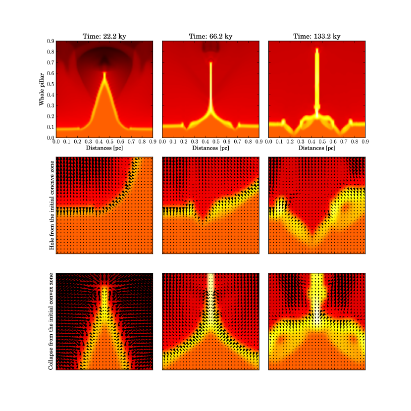
Figure 8: Zoom on the ionization of convex and concave zone in the w/h = 0.9 simulation between 22 and 132 ky. Arrows represent the velocity field projected in the x-y plane.

A closer look at the simulations (see Fig. 8) shows that the motions perpendicular to the propagation direction are shaping the structures. These motions are triggered by the initial curvature of the structure, two cases are distinguished, an initially convex zone and a initially concave zone. A shock front on a convex zone will trigger its collapse, it is the phenomenon which takes place in the radiation driven implosion scenario and here at the head of the initial structure. The curvature of the initial structure leads to lateral convergent shocks that collide on themselves. However the ionization of a concave zone is quite different, it will dig a hole in the medium, and the gas is pushed away lateraly. The velocity fields in Fig. 8 illustrate these phenomena, on a initially convex zone the velocities point inwards and lead to the collapse of the central structure whereas on the initially concave zone at the base they point outwards and dig a hole in the media. These phenomena are at the origin of the size and mass increase. Indeed, the collapse of the structure takes more time if the structure is wide, therefore it will be accelerated down longer, explaining the difference of vertical speed of the heads of the pillars seen in Fig. 7. Besides, the holes on each side of the pillar (see Fig. 8) gather the gas at the base of the pillar, explaining the mass increase in Fig. 7.

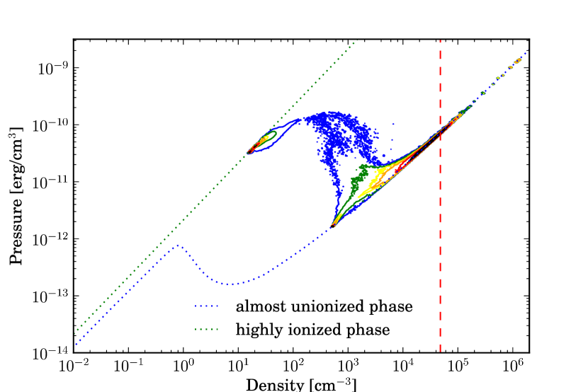
Figure 9: 2D plot of the mass fraction at a given density and pressure for the w/h = 0.9 simulation at the end of the simulation (554 ky). Blue to black contours are increasing mass fraction contours (blue: 1E-6, green: 1E-5, yellow: 5E-5, orange: 1E-4, red: 5E-4, black: 2E-3). The dashed-red line is the maximum density achieved in a plan-parallel 1D simulation : 4.8$\times$10⁴ cm³. The total mass at a density above this limit is around 10 solar masses

Besides the mass increase, there is an important density gain. The mass histogram in the pressure-density plane in Fig. 9 shows that the compression due to the heating from UV radiation increases the pressure of one order of magnitude from the initial state which is at a density of 500 cm³ and at a pressure of 10^-12 erg/cm³. The gas is then distributed in two phases at equilibrium, hot-ionized on the green-dashed straight line and cold-dense-unionized on the blue dashed curve. The gas in transition between them is seen with the blue contour. A 1D simulation of the collect and collapse process can increase the density up to 5$\times$10⁴ cm³, this limit is drawn with the red dashed line in Fig. 9. The mass at the base of the pillar, due to the holes from the initial concave parts and from the collapse of the lateral shocks, leads to a density enhancement of 1-2 orders of magnitude. Although the structures in our simulations are still slightly under their Jeans lengths, this process has a better chance to trigger star formation at the base of the pillars than the simple collect and collapse scenario.

3.2 From density modulations to pillars

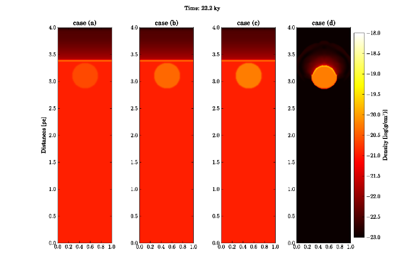
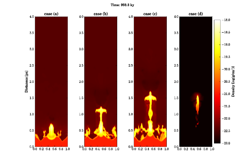
Figure 10: Density cuts of four simulations of an ionization front propagation on clumps (0.5 parsec in diameter). The UV flux at the top of the box is 10⁹ photons per second per square centimetre, the box is 4x2x2 parsecs (half of the cut is shown, only the central parsec of the simulation box). The last simulation (case(d)) is an isolated spherical clump of constant density 1000 cm³, the three others are clumps in a homogeneous medium of density 500 cm³. The clumps have densities of 1000 for case (a), 1750 for case (b) and 2500 cm³ for case (d).

Clouds have irregular shapes but they have also unhomogeneities. Therefore, after this study of interface modulations, we consider density modulations that we call clumps hereafter (with no reference to an observational definition). We define them as regions of constant overdensity. Figure 10 shows the different cases we studied. The three first cases are clumps in a homogeneous cold cloud, with a density contrast of respectively 2, 3.5 and 5 and the last one corresponds to the radiation driven implosion scenario, the clump is “isolated” in a hot low-density medium so that the shock forms directly on the structure, the density in the clump is the same as the one with a density contrast of 5. In all cases the clumps are at pressure equilibrium with the surrounding matter.

In the isolated case, the shock forms at the surface of the clump and the shell is therefore initially curved by the shape of the clump with a w/h ratio of 2. This roughly corresponds to the wider case studied in sect. 3.1. Since the shock is curved, it will collapse on itself and form a pillar-like structure, this case was studied in detail by Mackey & Lim (2010); Gritschneder et al. (2009). However, with a widht/heigh ratio of 2 the structure is quite small and look quite similar to the w/h=2 case of the previous section. However, since it is isolated, the accumulation of mass process at the base identified in the previous section can not take place.

In the three other cases, the shell is flat when it is formed, therefore the outcomes of the simulations are not so clear. When the clump is not dense enough (first case nH_clump/nH_cloud=2), it will not curve the shell enough to have lateral colliding shocks. Therefore in this case, there is no head in the final structure which is very small (i.e comparable to the initial clump size). In the two other simulations (nH_clump/nH_cloud=3.5 and 5), the clumps curve the shell enough to trigger the collision of vertical shocks thereby forming an elongated pillar. This is very close to what we observed previously on interface modulations. Besides, we can identify on the final snapshots a base for the pillar-structures formed by lateral holes in the cloud and the associated accretion mass process discussed above.

The importance of the curvature effect can be emphasized by comparing the isolated case and the nH_clump/nH_cloud=5 case. In both cases the density of the clump is the same, however when the shell is formed flat on a homogeneous medium, the dense clump will resist the shock to form an elongated modulation on the shock surface. In the isolated case, the shock is formed instantaneously curved on the structure with a w/h ratio of 2. Furthermore, contrary to the isolated case, the structures will grow in mass and size because of the connection with the cloud. These effects result in a final 0.5-parsec-long pillar for the isolated case whereas the final structure in the nH_clump/nH_cloud=5 case is 1.5 parsec long. The driving process to form a pillar is how the matter distribution is able to first curve the shell and then to feed the base of the pillar by the hole mechanism identified in sect. 3.1 (the holes are clearly visible in the final snapshots in Fig. 10).

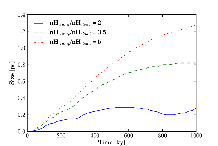
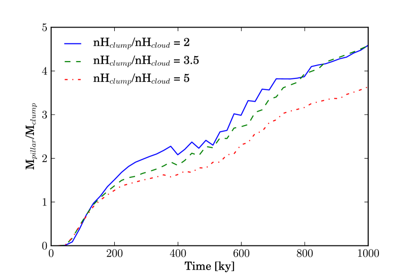
Figure 11: Monitoring of the size (top) and the mass (bottom) of pillars identified in Fig. 10. The size is calculated by the difference of the average position of the ionisation front and the its position at the centre of the y-z plane (head of the initial structure). The mass is calculated in a box between the two vertical positions defined to calculated the size and with a width defined by the width of the initial structure and is normalized by the mass of the initial clump.

The size evolution and the mass evolution of the pillars are comparable to the modulated-interface case. However the evolution is not linear due to the initial conditions. Indeed, there is a first phase in which the ionization front is curved and stretched verticaly around the clump when its propagation is slowed down by the overdensity. At this point (around 200 ky) the physical situation is comparable to the interface-modulated case, the ionization front is curved around a ”hill”. It also explains why we choose to do a longer simulation for the density-modulated case, it allows us to compare both cases at a ”physically equivalent” state at the end. When the lateral shocks collide around the hill, the pillar captures a bit more than the mass of the initial clump and its mass increase slows down. This phase occurs around 300 ky and can be clearly identified in Fig. 11. Then the mass increases due to the accumulation of matter at the base of the pillar. The process is less linear than in the interface-modulated case.

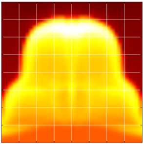
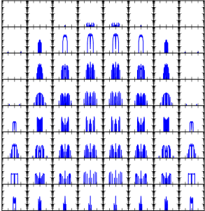
Figure 12: nH_clump/nH_cloud=5 simulation at t=222 ky. Left: column density on a 0.4x0.4x0.4 pc³ box around the pillar structure in a face-on geometry. Right: mass-weighted histogram of the line of sight velocity in the same box (similar to optically-thin observational line spectra). Each spectrum is made on a square of 0.05x0.05 pc² drawn on the column density map. The spectra are drawn between -4 and 4 km/s in 80 bins (horizontal axis) and the mass between 10^-4 and 1 solar mass (vertical axis in log scale). The lateral shocks can be clearly identified in the double wings spectra leading to a very broad line width.

4 Observational signature

The two sections above present how pillars can be formed on a density or interface modulated region of the molecular cloud. These pillars are connected to the cloud, increasing in size and mass with time. However these variations can not be observed. A potentially observational signature to study is the structure of the line of sight velocity. We use the same method as Gritschneder et al. (2010). We define a grid of squares of 0.05x0.05 pc² along the pillar and we bin the line of sight velocity in each square (see Fig. 12, 13 and 14). We use the simulation with the densest clump to study the line of sight velocity structure but the following results are generic. At t=222 ky (Fig. 12), the lateral shocks can be clearly identified in the broad line spectrum. There are two components, a positive one coming towards us and a negative one going away. At this time the shell is curved around a hill which is comparable to the situation we got in the interface-modulated scenario after a short time.

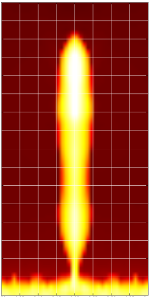
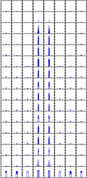
Figure 13: nH_clump/nH_cloud=5 simulation at t=444 ky. Same plots as Fig. 12. The lateral shocks collided and cannot been identified anymore.

At t=444 ky (Fig. 13), the lateral shocks have collided resulting in a small line width for the histograms. The whole pillar is narrow and evacuates the pressure through radiative cooling and expansion to reach the equilibrium defined for the cold phase in figure 9. There is two dense part in the pillar: the head in which the matter of the clump has been accumulated and the base at the point where the lateral shocks have closed. It will resist the ionization because it is dense enough and matter is starting to accumulate at the base.

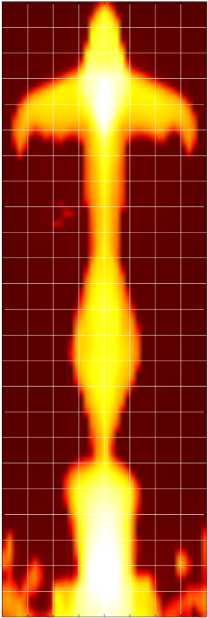
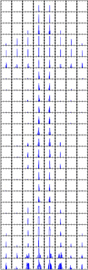
Figure 14: nH_clump/nH_cloud=5 simulation at t=998 ky. Same plots as Fig. 12. The line width is very small compared to the snapshots at t=222 ky.

At t= 998 ky (Fig. 14), matter has accumulated at the base of the pillar, based on the process that was identified in Fig. 8. The line of sight velocity histograms have still a small line width compared to Fig.12. This phenomenon is not specific to clumps simulations, the same analysis on the interface modulated simulation (aspect ratio of 0.9) in Fig. 15 and Fig. 16 shows similar results but at an earlier stage. The interface modulated simulation presents double-wing velocity spectra around t=22.2 ky whereas the clumpy simulation presents these spectra around t=222 ky when the shock is curved around a hill. The double-wing structure of the velocity spectra is therefore a signature of the lateral shocks which are going to collide and a signature of the early stage of a forming pillar.

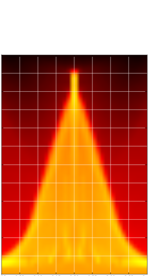
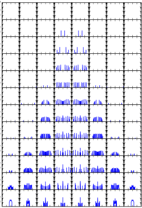
Figure 15: w/h=0.9 simulation at t=22.2 ky (first column in Fig. 8). The shock just formed on the modulation, the line width and the double-wing structure is comparable to Fig. 12

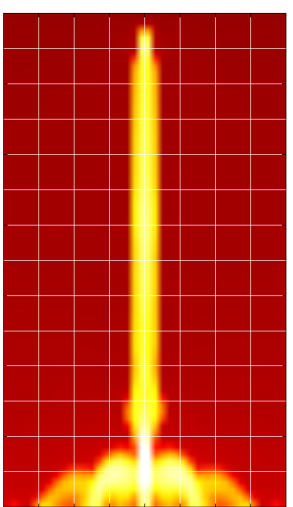
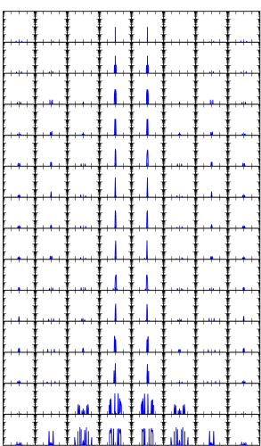
Figure 16: w/h=0.9 simulation at t=133.2 ky (third column in Fig. 8). The shock collided lateraly and the line width is small as in Fig. 13

The previous analysis can be applied to the different simulations presented in this paper without noticable change to our conclusion. We also changed some physical conditions and parameters. We added a constant external gravitational field, included self-gravity, doubled the resolution without global changes in the morphology of the final structures. We also changed the flux to an higher value (from 10⁹ to 5$\times$10⁹ photons/s/cm²) and the structures are similar but evolve faster as seen by Gritschneder et al. (2009). The shell speed $c_{shell}$ is proportional to $F_{\gamma}^{1/4}$ (see Eq. 16 and Eq. 18) therefore multiplying the flux by five increases the shell speed by 50% and the whole simulation evolves 50% faster. In all these situations, pillars form by the lateral collision of a curved shocked surface and the double-wing spectrum is always visible before the shocks collide.

5 Conlusion and discussion

We have presented a new scenario for the formation of structures at the edge of HII regions and shown that:

1. A curved shock ahead of an ionization front can lead to a pillar if it is curved enough to collide lateraly on itself.

2. This pocess is very efficient to form stable growing pillar, the narrower the initial structure, the more curved the front and the longer the pillar.

3. Lateral gas flows can result in a density enhancement at the base of the pillars of 1-2 orders of magnitude compared to the collect and collapse scenario.

4. When the shock is first formed flat, it can be curved by enough-dense clumps and leads to pillars. On isolated clumps (Radiation Driven Implosion) , the shock is naturally curved by the form of the clump but the resulting structure has a constant size and mass.

5. The double-wing line spectra of the line-of-sight velocity is a signature of the lateral collision of the shock, and hence is a signature of the early stage of the formation of a pillar. It can be used as an observational signature for this new scenario.

Various aspects of shocks orientation have been considered by other authors. Oblique shocks have previously been studied by Chevalier & Theys (1975) and cylindrical shocks by Kimura, Toshiya & Tosa (1990). These effects have been further explored in the context of 2D turbulent simulations (see Elmegreen et al., 1995). However these studies focus on the effects of curvature on clumps enhancement. In this work, we have shown that shocks need to be enough curved to collide on themselves in order to form a pillar like structure.

At the edge of HII regions, the structure of the line-of-sight velocity can be investigated using radiotelescopes and suitable molecules tracing the dynamic, to detect the double-wing spectra on gas hills and thus nascent pillars. If a gas overdensity is detected at the top of the hill (e.g. using Herschel data), the shock curvature could be attributed to the presence of an initial clump, if not to the curvature of an initial interface.

In this study, curved shocks have been generated using either density or interface modulations on a pc scale and in a very simplified situation. However, we expect that the physical processes discussed in this paper can also be applied to more realistic situations where the ionization front interact with a turbulent interstellar medium. In this case the density fluctuations are much more complex, but the same mechanism should be at work to describe pillar formation. These turbulent situations will be studied in a forthcoming paper in which the interplay between shock curvature and turbulence will be studied to see its impact on star formation rates at the edge of HII regions.

References

- Andersen et al. (2004) Andersen, M., Knude, J., Reipurth, B., et al. 2004, Astronomy and Astrophysics, 414, 969
- Arthur et al. (2011) Arthur, S. J., Henney, W. J., Mellema, G., De Colle, F., & Vázquez-Semadeni, E. 2011, Monthly Notices of the Royal Astronomical Society, -1, no
- Audit & Hennebelle (2005) Audit, E. & Hennebelle, P. 2005, Astronomy and Astrophysics, 433, 1
- Bertoldi (1989) Bertoldi, F. 1989, The Astrophysical Journal, 346, 735
- Bisbas et al. (2009) Bisbas, T. G., Wünsch, R., Whitworth, A. P., & Hubber, D. A. 2009, Astronomy and Astrophysics, 497, 649
- Black (1981) Black, . 1981, Royal Astronomical Society, 197, 553
- Bowler et al. (2009) Bowler, B. P., Waller, W. H., Megeath, S. T., Patten, B. M., & Tamura, M. 2009, The Astronomical Journal, 137, 3685
- Chevalier & Theys (1975) Chevalier, R. A. & Theys, J. C. 1975, The Astrophysical Journal, 195, 53
- Dale & Bonnell (2011) Dale, J. E. & Bonnell, I. 2011, Monthly Notices of the Royal Astronomical Society, 414, no
- Dale et al. (2007) Dale, J. E., Bonnell, I. A., & Whitworth, A. P. 2007, Monthly Notices of the Royal Astronomical Society, 375, 1291
- Deharveng et al. (2010) Deharveng, L., Schuller, F., Anderson, L. D., et al. 2010, Astronomy & Astrophysics, 523, A6
- Elmegreen et al. (1995) Elmegreen, B. G., Kimura, T., & Tosa, M. 1995, The Astrophysical Journal, 451, 675
- Elmegreen & Lada (1977) Elmegreen, B. G. & Lada, C. J. 1977, The Astrophysical Journal, 214, 725
- González et al. (2007) González, M., Audit, E., & Huynh, P. 2007, Astronomy and Astrophysics, 464, 429
- Gritschneder et al. (2009) Gritschneder, M., Naab, T., Burkert, A., et al. 2009, Monthly Notices of the Royal Astronomical Society, 393, 21
- Gritschneder et al. (2010) Gritschneder, ., Burkert, A., Naab, T., & Walch, S. 2010, The Astrophysical Journal, 723, 971
- Jiang et al. (2002) Jiang, Z., Yao, Y., Yang, J., et al. 2002, The Astrophysical Journal, 577, 245
- Kessel-Deynet & Burkert (2003) Kessel-Deynet, O. & Burkert, A. 2003, Monthly Notices of the Royal Astronomical Society, 338, 545
- Kimura, Toshiya & Tosa (1990) Kimura, Toshiya & Tosa, M. 1990, Royal Astronomical Society, 245, 365
- Krumholz et al. (2007) Krumholz, M. R., Stone, J. M., & Gardiner, T. A. 2007, The Astrophysical Journal, 671, 518
- Lefloch et al. (2002) Lefloch, B., Cernicharo, J., Rodriguez, L. F., et al. 2002, The Astrophysical Journal, 581, 335
- Lefloch, B. & Lazareff (1994) Lefloch, B. & Lazareff, B. 1994, Astronomy and Astrophysics (ISSN 0004-6361), 289, 559
- Lora et al. (2009) Lora, V., Raga, A. C., & Esquivel, A. 2009, Astronomy and Astrophysics, 503, 477
- Mackey & Lim (2010) Mackey, J. & Lim, A. J. 2010, Fluid Dynamics, 730, 714
- Mellema et al. (2006) Mellema, G., Arthur, S. J., Henney, W. J., Iliev, I. T., & Shapiro, P. R. 2006, The Astrophysical Journal, 647, 397
- Price et al. (2010) Price, D. J., Bate, M. R., Bertin, G., et al. 2010, Magnetic fields and radiative feedback in the star formation process, Vol. 1242, 205–218
- Purcell et al. (2009) Purcell, C. R., Minier, V., Longmore, S. N., et al. 2009, Astronomy and Astrophysics, 504, 139
- Reach et al. (2004) Reach, W. T., Rho, J., Young, E., et al. 2004, The Astrophysical Journal Supplement Series, 154, 385
- Schneider et al. (2010) Schneider, N., Motte, F., Bontemps, S., et al. 2010, Astronomy and Astrophysics, 518, L83
- Smith et al. (2000) Smith, N., Egan, M. P., Carey, S., et al. 2000, The Astrophysical Journal, 532, L145
- Spitzer (1978) Spitzer, L. 1978, Physical Processes in the Interstellar Medium (Wiley-VCH)
- Strömgren (1939) Strömgren, B. 1939, The Astrophysical Journal, 89, 526
- Walborn et al. (2002) Walborn, N. R., Maíz-Apellániz, J., & Barbá, R. H. 2002, The Astronomical Journal, 124, 1601
- Williams et al. (2001) Williams, R. J. R., Ward-Thompson, D., & Whitworth, A. P. 2001, Monthly Notices of the Royal Astronomical Society, 327, 788
- Wolfire et al. (1995) Wolfire, M. G., Hollenbach, D., McKee, C. F., Tielens, A. G. G. M., & Bakes, E. L. O. 1995, The Astrophysical Journal, 443, 152
- Wolfire et al. (2003) Wolfire, M. G., McKee, C. F., Hollenbach, D., & Tielens, A. G. G. M. 2003, The Astrophysical Journal, 587, 278