Abstract

In this paper a model describing fermions and gauge field localized on a domain wall is considered. The zero-mode sector of the model reproduces four-dimensional spinor electrodynamics. It is shown that in the resulting four-dimensional effective theory the lowest-order renormalized amplitude of the elastic $\gamma\gamma$ scattering process is divergent due to the contributions of higher modes and thus such a scenario can not be considered as a realistic mechanism for fields localization on a domain wall.

1 Introduction

Models with extra dimensions offer many interesting possibilities for resolving existing problems in theoretical physics. There are different approaches in such theories, the most popular now being brane world models. In many brane world models it is assumed that matter is localized on a brane, embedded into multidimensional space-time, but very often the particular mechanism of localization is not considered explicitly. Indeed, the mechanism of localization of massless fermions is known for a long time, as it was proposed in [1]. As for bosons, especially gauge fields, there are also some ways to localize them. The most known is the mechanism proposed in [2] (see also [3]), where the ideas of confinement were used to trap the gauge fields. Another approach is to make the wave functions of massless four-dimensional gauge bosons constant in extra dimensions (to ensure the universality of charge, which is important for constructing realistic models, see [4]), but normalizable. The latter can be achieved either by introducing more than one extra dimension in models with warped geometry [5], or by considering an additional overall coupling of the gauge field to an extra scalar field, for example, dilaton field [6] (or just to a weight function depending explicitly on the extra coordinate as in [7]), in five-dimensional models. But it should be necessarily noted that there were earlier attempts to localize gauge fields on a domain wall, see, for example, [8].

In this paper we consider a model with both gauge and spinor fields lowest modes localized on a domain wall. We use the mechanism of consistent localization of massive fermions on a domain wall, which is based on the well-known Rubakov-Shaposhnikov mechanism [1] and proposed in [9] (but we consider it in the absence of gravity). This mechanism has already been discussed and utilized in different models [10, 11, 12, 13]. We present an explicit solution for the zero fermionic mode, which looks as an ordinary four-dimensional massive fermion, as well as for the excited modes, which also represent four-dimensional massive fermions. We also present a mechanism of localization of gauge vector fields on a domain wall (again in the absence of gravity), which is motivated by the results of [6, 7, 8] and utilizes the ideas presented there: an overall coupling of the gauge field to the scalar field to make the wave function of the gauge field normalizable [6] and taking this scalar field to be the one which forms the domain wall proper [8] (it should be noted that the same idea in connection with localization of gauge fields on thick branes has been recently utilized in [14]). We show explicitly that both mechanisms lead to quite interesting results: for bosons, as well as for fermions, there exist nonzero mass gaps between the lowest (zero) massive or massless localized modes and the other localized and nonlocalized modes which arise from the five-dimensional theory. This allows one to consider a combination of these mechanisms and to construct a simple five-dimensional model, involving two five-dimensional fermions, interacting with five-dimensional $U(1)$ gauge field, whose localized sector represents ordinary four-dimensional spinor electrodynamics. But it appears that such a theory after a renormalization leads to infinite amplitudes of some processes involving only the lowest localized modes in initial and final states (the $\gamma\gamma\to\gamma\gamma$ scattering is considered, which is well behaved in ordinary four-dimensional QED). This happens because of a contribution of the modes from the continuous spectrum. Thus, such a model can not be considered as realistic for describing matter fields localization on a brane or a domain wall and one should look for more consistent scenarios.

2 Localized massive fermions

2.1 Localization mechanism

The well-known mechanism of localization of fermions is the Rubakov-Shaposhnikov mechanism [1]. It describes a five-dimensional fermion field interacting with a background scalar field admitting, for example, the kink solution

$$\Phi_{0}=\frac{m}{\sqrt{\lambda}}\tanh\left(\frac{m}{\sqrt{2}}z\right).$$ (1)

The mechanism allows one to get a localized four-dimensional chiral mode of the fermion. The problem is that the localized fermion is massless, whereas it is clear that there should be localized modes, describing massive four-dimensional fermions, in order to represent real massive four-dimensional particles. Indeed, for the kink profile (1) of the scalar field the left fermion field (left from the four-dimensional point of view) behaves as

$$\Psi_{L}(x,z)\to C_{L}\psi_{L}(x)e^{-\frac{hm}{\sqrt{\lambda}}|z|}$$ (2)

at large $z$, whereas the right fermion field (right from the four-dimensional point of view) behaves as

$$\Psi_{R}(x,z)\to C_{R}\psi_{R}(x)e^{\frac{hm}{\sqrt{\lambda}}|z|}$$ (3)

at large $z$, i.e. its wave function grows at infinity for $C_{R}\neq 0$ and we should set $C_{R}=0$. Meanwhile, it is necessary to have both chiralities, preferably with the same wave functions, in order to describe massive four-dimensional fermions, so one should introduce two five-dimensional fermion fields. One fermion field provides the localized left-handed component of the four-dimensional Dirac spinor, whereas another fermion field provides the localized right-handed component of the four-dimensional Dirac spinor. An interaction term of these fermion fields results in a four-dimensional mass term. To our knowledge, for the first time this mechanism was utilized in [9] when considering the behavior of matter in brane world models (i.e. taking into account the gravitational interaction). Then analogous constructions were used in [10] for explaining the origin of the three generations of the Standard Model fermions and in [12, 13] for constructing domain walls generated by a fermion self-interaction. Below we will recall this mechanism and examine some of its properties. We will show how it provides the existence of four-dimensional massive fermions localized on a domain wall.

Let us take the five-dimensional action corresponding to the model of [9], but in the absence of gravity (see also the simple model discussed in the beginning of [12]). In our notations this action has the form:

$$S=\int\left[i\bar{\Psi}_{1}\Gamma^{M}\partial_{M}\Psi_{1}-h\Phi\bar{\Psi}_{1}\Psi_{1}+i\bar{\Psi}_{2}\Gamma^{M}\partial_{M}\Psi_{2}+h\Phi\bar{\Psi}_{2}\Psi_{2}-\right.$$ (4)

$$\left.-M\left(\bar{\Psi}_{1}\Psi_{2}+\bar{\Psi}_{2}\Psi_{1}\right)\right]d^{4}xdz,$$

where $\Psi_{1}$ and $\Psi_{2}$ are different five-dimensional fermion fields, $h>0$, $M=0,..,4$, $\Gamma^{\mu}=\gamma^{\mu}$, $\Gamma^{4}=i\gamma^{5}$. The equations of motion coming from this action have the form

$$i\gamma^{\mu}\partial_{\mu}\Psi_{1}-\gamma^{5}\Psi^{\prime}_{1}-h\Phi_{0}\Psi_{1}-M\Psi_{2}=0,$$ (5)

$$i\gamma^{\mu}\partial_{\mu}\Psi_{2}-\gamma^{5}\Psi^{\prime}_{2}+h\Phi_{0}\Psi_{2}-M\Psi_{1}=0,$$ (6)

where ^′ denotes $\partial_{4}$ and $\Phi_{0}(z)$ is a domain wall profile (see equations (1.9) and the subsequent discussion in [12]). Let us take the following form of the solution to these equations:

$$\Psi_{1}(x,z)=f(z)\psi_{L}(x),\qquad\gamma^{5}\psi_{L}=\psi_{L},$$ (8)

$$\Psi_{2}(x,z)=f(z)\psi_{R}(x),\qquad\gamma^{5}\psi_{R}=-\psi_{R}.$$

Substituting (8), (8) into (5), (6) we easily get:

$$\Psi_{1}(x,z)=Ce^{-h\int_{0}^{z}\Phi_{0}(z^{\prime})dz^{\prime}}\psi_{L}(x),\qquad i\gamma^{\mu}\partial_{\mu}\psi_{L}-M\psi_{R}=0,$$ (9)

$$\Psi_{2}(x,z)=Ce^{-h\int_{0}^{z}\Phi_{0}(z^{\prime})dz^{\prime}}\psi_{R}(x),\qquad i\gamma^{\mu}\partial_{\mu}\psi_{R}-M\psi_{L}=0,$$ (10)

where $C$ is a normalization constant. The four-dimensional equations in (9) and (10) can be combined into one equation by taking

$$\psi_{L}(x)+\psi_{R}(x)=\psi(x)$$

and we get

$$i\gamma^{\mu}\partial_{\mu}\psi-M\psi=0.$$ (11)

The latter equation is nothing but the Dirac equation for a massive fermion. Thus, we get the localized mode, which describes a massive four-dimensional fermion. This massive four-dimensional fermion appears to be the superposition of the zero modes of the two initial five-dimensional fermions.

The corresponding four-dimensional effective action for this mode can be easily obtained and has the form

$$S=C^{2}\int e^{-2h\int_{0}^{z}\Phi_{0}(z^{\prime})dz^{\prime}}dz\int\left(i\bar{\psi}\gamma^{\mu}\partial_{\mu}\psi-M\bar{\psi}\psi\right)d^{4}x.$$ (12)

If $C$ is chosen in a proper way, we get a canonically-normalized four-dimensional effective action having the standard form

$$S_{eff}=\int\left(i\bar{\psi}\gamma^{\mu}\partial_{\mu}\psi-M\bar{\psi}\psi\right)d^{4}x.$$ (13)

Of course, this mechanism, as well as the original mechanism [1], can be utilized not only with the kink profile of the background scalar field, but with any background scalar field profile suitable for obtaining normalizable wave functions of fermions.

2.2 Mass gap and excited fermion states

Now let us turn to examining the properties of this mechanism. Indeed, it is not evident that the localized mode presented in the previous section is the lowest one and that there is a nonzero mass gap between the lowest mode and the next possible localized mode or the continuous spectrum. To this end let us obtain the second order differential equations for the spinors $\Psi_{1}$ and $\Psi_{2}$. This can be done by the standard technique and we obtain

$$-\partial^{\mu}\partial_{\mu}\Psi_{1}-M^{2}\Psi_{1} = -\Psi^{\prime\prime}_{1}-h\Phi_{0}^{\prime}\gamma^{5}\Psi_{1}+h^{2}\Phi_{0}^{2}\Psi_{1},$$ (14)

$$-\partial^{\mu}\partial_{\mu}\Psi_{2}-M^{2}\Psi_{2} = -\Psi^{\prime\prime}_{2}+h\Phi_{0}^{\prime}\gamma^{5}\Psi_{2}+h^{2}\Phi_{0}^{2}\Psi_{2}.$$ (15)

For $M=0$ the first of these equations has exactly the same form as the one which can be obtained in the model [1] with just one five-dimensional spinor. This is enough to make some statements about other possible localized modes – we know that in the model [1] there may be (or may not be) other localized states with larger masses and that there is a nonzero mass gap between the lowest mode and the continuous spectrum. In the model discussed here we can also easily obtain analogous estimates. To this end one should solve the equation for the wave function, coming from (14) (equation (15) also gives the same equation):

$$\left(\mu^{2}-M^{2}\right)f(z)=-f^{\prime\prime}(z)\mp h\Phi_{0}^{\prime}f(z)+h^{2}\Phi_{0}^{2}f(z),$$ (16)

where $\mp$ comes from $\gamma^{5}$ acting on the left-handed and right-handed fermions respectively. For the kink profile (1) of the background field we get

$$\left(\mu^{2}-M^{2}-h^{2}\frac{m^{2}}{\lambda}\right)f(z)=-f^{\prime\prime}(z)-\frac{h^{2}\frac{m^{2}}{\lambda}\pm h\frac{m^{2}}{\sqrt{2\lambda}}}{\cosh^{2}\left(\frac{m}{\sqrt{2}}z\right)}f(z).$$ (17)

It is the standard Schrödinger-type equation with the known solution – the eigenvalues, corresponding to the localized modes, are (see, for example, [15])

$$\mu^{2}=M^{2}+\frac{\sqrt{2}hm^{2}}{\sqrt{\lambda}}\left(n+\frac{1}{2}\mp\frac{1}{2}\right)-\frac{m^{2}}{2}\left(n+\frac{1}{2}\mp\frac{1}{2}\right)^{2},\qquad n\leq\frac{\sqrt{2}h}{\sqrt{\lambda}}-\frac{1}{2}\pm\frac{1}{2}.$$ (18)

Here $n=0,1,2,...$ and we suppose that $\frac{\sqrt{2}h}{\sqrt{\lambda}}\geq 1$. The lowest mode, as expected, has the mass $\mu_{0}=M$. The next eigenvalue is

$$\mu_{1}=\sqrt{M^{2}+\frac{m^{2}}{\sqrt{2}}\left(\frac{2h}{\sqrt{\lambda}}-\frac{1}{\sqrt{2}}\right)}.$$

Thus, the mass gap is at least

$$\Delta\mu=\sqrt{M^{2}+\frac{m^{2}}{\sqrt{2}}\left(\frac{2h}{\sqrt{\lambda}}-\frac{1}{\sqrt{2}}\right)}-M.$$ (19)

Now let us show how the excited modes look like in the scenario under consideration. Let us consider the $n$-th Kaluza-Klein level, $n\geq 1$, and suppose that it contains particles with the same four-dimensional mass $\mu$. It follows from (16) that the wave function $f(z)$ of the fermions, for which $\gamma^{5}\Psi_{1}=\Psi_{1},\,\gamma^{5}\Psi_{2}=-\Psi_{2}$ hold, fulfills the equation

$$\left(\mu^{2}-M^{2}\right)f(z)=-f^{\prime\prime}(z)-h\Phi_{0}^{\prime}f(z)+h^{2}\Phi_{0}^{2}f(z),$$ (20)

whereas the wave function $\tilde{f}(z)$ of the fermions, for which $\gamma^{5}\Psi_{1}=-\Psi_{1},\,\gamma^{5}\Psi_{2}=\Psi_{2}$ hold, fulfills the equation

$$\left(\mu^{2}-M^{2}\right)\tilde{f}(z)=-{\tilde{f}}^{\prime\prime}(z)+h\Phi_{0}^{\prime}\tilde{f}(z)+h^{2}\Phi_{0}^{2}\tilde{f}(z).$$ (21)

It is not difficult to show that equations (20) and (21) can be obtained from the following system of equations

$$f^{\prime}+h\Phi_{0}f=(\mu+M){\tilde{f}},$$ (22)

$${\tilde{f}}^{\prime}-h\Phi_{0}{\tilde{f}}=-(\mu-M)f,$$ (23)

which will be used below. Equations (20) and (21) suggest the decomposition for the five-dimensional spinors $\Psi_{1}$ and $\Psi_{2}$:

$$\Psi_{1}(x,z)=f(z)\psi_{L}(x)+\frac{\tilde{f}(z)}{D}\hat{\psi}_{R}(x),$$ (24)

$$\Psi_{2}(x,z)=f(z)\psi_{R}(x)-\frac{\tilde{f}(z)}{D}\hat{\psi}_{L}(x),$$ (25)

where $D^{2}=\int{\tilde{f}}^{2}dz$, $\psi_{L}=\gamma^{5}\psi_{L}$, $\psi_{R}=-\gamma^{5}\psi_{R}$, $\hat{\psi}_{L}=\gamma^{5}\hat{\psi}_{L}$, $\hat{\psi}_{R}=-\gamma^{5}\hat{\psi}_{R}$. We also impose the normalization condition $\int f^{2}dz=1$, which results in $D^{2}=\frac{\mu-M}{\mu+M}$ (the value of $D$ can be obtained from equations (22), (23).

Substituting decomposition (24), (25) into action (4), taking into account (22), (23) and then integrating over the coordinate of the extra dimension, we get the effective four-dimensional action

$$S_{eff}=\int d^{4}x\left(i\bar{\psi}\gamma^{\mu}\partial_{\mu}\psi+i\bar{\hat{\psi}}\gamma^{\mu}\partial_{\mu}\hat{\psi}-M(\bar{\psi}\psi-\bar{\hat{\psi}}\hat{\psi})-\sqrt{\mu^{2}-M^{2}}\left(\bar{\psi}\hat{\psi}+\bar{\hat{\psi}}\psi\right)\right),$$ (26)

where $\psi=\psi_{L}+\psi_{R}$, $\hat{\psi}=\hat{\psi}_{L}+\hat{\psi}_{R}$. The mass matrix can be diagonalized with the help of the rotation

$$\psi(x) = \psi_{1}(x)\cos(\theta)+\psi_{2}(x)\sin(\theta),$$ (27)

$$\hat{\psi}(x) = \psi_{1}(x)\sin(\theta)-\psi_{2}(x)\cos(\theta),$$ (28)

where $\tan(2\theta)=\frac{\sqrt{\mu^{2}-M^{2}}}{M}$. The last step is to make the redefinition $\psi_{2}\to\gamma^{5}\psi_{2}$ in order to get the conventional sign of the mass term of the four-dimensional fermion $\psi_{2}$. Finally, we get

$$S_{eff}=\int d^{4}x\sum\limits_{i=1}^{2}\left[i\bar{\psi}_{i}\gamma^{\mu}\partial_{\mu}\psi_{i}-\mu\bar{\psi}_{i}\psi_{i}\right].$$ (29)

The equation for the function $f$ for the kink profile of the background scalar field looks like

$$\left(\mu^{2}-M^{2}-h^{2}\frac{m^{2}}{\lambda}\right)f(z)=-f^{\prime\prime}(z)-\frac{h^{2}\frac{m^{2}}{\lambda}+h\frac{m^{2}}{\sqrt{2\lambda}}}{\cosh^{2}\left(\frac{m}{\sqrt{2}}z\right)}f(z).$$ (30)

We know one solution to this equation – it is simply given by (9), (10), $\mu=M$ in this case and from (22) we get ${\tilde{f}}\equiv 0$. Indeed, this is the lowest localized mode.

The next localized solution to equation (30) has the form

$$f_{1}=C\frac{\sinh\left(\frac{m}{\sqrt{2}}z\right)}{\cosh^{\alpha}\left(\frac{m}{\sqrt{2}}z\right)},$$ (31)

where $\alpha=\frac{h\sqrt{2}}{\sqrt{\lambda}}$ and $C$ is the normalization constant. The four-dimensional mass of this mode is $\mu_{1}^{2}=M^{2}+m^{2}\left(\frac{\sqrt{2}h}{\sqrt{\lambda}}-\frac{1}{2}\right)$. From (22) we get

$$\tilde{f}_{1}=C\frac{m}{\sqrt{2}(\mu_{1}+M)\cosh^{\alpha-1}\left(\frac{m}{\sqrt{2}}z\right)}.$$ (32)

Of course, there can be other localized modes, their number $N$ is defined by (see (18))

$$N=\textrm{max}\left\{n\in\mathbb{Z}\left|\right.0<n<1+\frac{\sqrt{2}h}{\sqrt{\lambda}}\right\}.$$ (33)

They are solutions to equations (30) and (22).

With the help of (22) and (23) it is not difficult to show that the following orthogonality conditions are fulfilled in the general case

$$\int f_{n}f_{k}dz=0,\qquad\int{\tilde{f}_{n}}{\tilde{f}_{k}}dz=0,\qquad n\neq k.$$ (34)

This is also valid for the modes from the continuous spectrum.

It should be noted that in general there exist two linearly independent solutions to equation (20) corresponding to each eigenvalue $\mu$ (the same is valid for equation (21) also). For the modes from the discrete spectrum one solution is normalizable, whereas another one grows at infinity and should be set to zero. Thus, in this case only one solution to each equation survives. But for the modes from the continuous spectrum both solutions to equation (20) (as well as to equation (21)) have a good behavior at infinity in the general case and thus both solutions should be taken into account (one can choose, say, odd and even solutions if $\Phi_{0}(z)$ is odd). We will use the notations $f_{(\mu,j)}$ and $\tilde{f}_{(\mu,j)}$, $j=1,2$, for these solutions to equations (20) and (21).

Thus, for the localized modes we can set

$$\int f_{n}f_{k}dz=\delta_{nk},$$ (35)

whereas for the modes from the continuous spectrum we set

$$\int f_{(\mu,j)}f_{(\mu^{\prime},j^{\prime})}dz=\delta(\mu-\mu^{\prime})\delta_{jj^{\prime}}.$$ (36)

Now let us obtain the full four-dimensional effective action for the fermions. To this end we substitute

$$\Psi_{1} = \sum\limits_{n=0}^{N}\left(f_{n}(z)\psi_{L}^{n}(x)+\frac{{\tilde{f}_{n}(z)}}{D_{n}}\hat{\psi}_{R}^{n}(x)\right)+$$

$$+ \sum\limits_{j=1}^{2}\int d\mu\left(f_{(\mu,j)}(z)\psi_{L}^{(\mu,j)}(x)+\frac{{\tilde{f}_{(\mu,j)}(z)}}{D_{(\mu)}}\hat{\psi}_{R}^{(\mu,j)}(x)\right),$$

$$\Psi_{2} = \sum\limits_{n=0}^{N}\left(f_{n}(z)\psi_{R}^{n}(x)-\frac{{\tilde{f}_{n}(z)}}{D_{n}}\hat{\psi}_{L}^{n}(x)\right)+$$

$$+ \sum\limits_{j=1}^{2}\int d\mu\left(f_{(\mu,j)}(z)\psi_{R}^{(\mu,j)}(x)-\frac{{\tilde{f}_{(\mu,j)}(z)}}{D_{(\mu)}}\hat{\psi}_{L}^{(\mu,j)}(x)\right),$$

where $\tilde{f}_{0}\equiv 0$, into (4) and after some algebra (including the rotation (27), (28) with $\tan(2\theta_{n})=\frac{\sqrt{\mu_{n}^{2}-M^{2}}}{M}$, $n\geq 1$, $\tan(2\theta_{(\mu,j)})=\frac{\sqrt{\mu^{2}-M^{2}}}{M}$ at each Kaluza-Klein level) we get the four-dimensional action

$$S_{eff}=\int\left(i\bar{\psi}\gamma^{\nu}\partial_{\nu}\psi-M\bar{\psi}\psi\right)d^{4}x+$$ (39)

$$+\sum\limits_{i=1}^{2}\left(\sum\limits_{n=1}^{N}\int\left(i\bar{\psi}^{n}_{i}\gamma^{\nu}\partial_{\nu}\psi^{n}_{i}-\mu_{n}\bar{\psi}^{n}_{i}\psi^{n}_{i}\right)d^{4}x+\right.$$

$$\left.+\sum\limits_{j=1}^{2}\int d\mu\int\left(i\bar{\psi}^{(\mu,j)}_{i}\gamma^{\nu}\partial_{\nu}\psi^{(\mu,j)}_{i}-\mu\bar{\psi}^{(\mu,j)}_{i}\psi^{(\mu,j)}_{i}\right)d^{4}x\right),$$

where $\psi$, $\psi^{n}_{i}$ and $\psi^{(\mu,j)}_{i}$ are the four-component spinors. We see that each Kaluza-Klein level, except the lowest one with $\mu_{0}=M$, contains two (discrete spectrum) or four (continuous spectrum) four-dimensional fermions with the equal masses $\mu$. The doubling parameterized by $i$ is of the same nature as that in the UED models, see, for example, [16].

We have shown that for the kink profile of the background scalar field the excited localized modes really exist and correspond to four-dimensional massive fermions. The continuous spectrum, as it can be seen from (17), starts at

$$\mu=\sqrt{M^{2}+\frac{h^{2}}{\lambda}m^{2}}.$$

Quite an interesting case is that with $\frac{h}{\sqrt{\lambda}}=\frac{1}{\sqrt{2}}$. In this case $\alpha=1$ in eqs. (31), (32) and, according to (33), there is only one localized mode with the mass $\mu_{0}=M$, the continuous spectrum starts at $\mu=\sqrt{M^{2}+\frac{m^{2}}{2}}$. Thus, for the mass gap we have

$$\Delta\mu=\sqrt{M^{2}+\frac{m^{2}}{2}}-M$$ (40)

and for $m\gg M$

$$\Delta\mu\approx\frac{m}{\sqrt{2}}.$$ (41)

Below for simplicity we will study this case $\frac{h}{\sqrt{\lambda}}=\frac{1}{\sqrt{2}}$.

Thus, we see that the model proposed in [9] provides us massive fermions, localized on a domain wall, and a nonzero mass gap between these modes and the subsequent continuous spectrum.

3 Localized U(1) gauge field

Now we turn to the gauge fields. We consider the simplest five-dimensional $U(1)$ gauge field. The corresponding five-dimensional action is chosen to be

$$S=-\int\xi^{2}\left(\Phi_{v}^{2}-\Phi^{2}\right)\frac{1}{4}F^{MN}F_{MN}d^{4}xdz,$$ (42)

where $F_{MN}=\partial_{M}A_{N}-\partial_{N}A_{M}$, $M,N=0,1,..,4$, here and below the parameter $\xi$ is chosen so that the dimension of $A_{M}$ is mass (like in a four-dimensional theory). We also suppose that the background solution is such that $A_{M}\equiv 0$, $\Phi(x,z)=\Phi_{0}(z)$ represents the domain wall, $\Phi\to\pm\Phi_{v}$ at $z\to\pm\infty$ and $\Phi_{v}^{2}-\Phi^{2}>0$.

Action (42) looks rather nonstandard because of the term $\Phi_{v}^{2}-\Phi^{2}$. Nevertheless, an analogous form of interaction (namely, $(\Phi_{v}^{2}-\Phi^{2})^{2}$) was discussed in [8] while constructing a mechanism of gauge field trapping on a domain wall and in [17] (see also [14]).

From the very beginning it is convenient to work in the gauge $A_{4}\equiv 0$. After imposing this gauge we are left with residual gauge transformations $A_{\mu}\to A_{\mu}-\partial_{\mu}\alpha$ with $\alpha(x,z)=\alpha(x)$.

Let us represent the field $A_{\mu}$ as

$$A_{\mu}(x,z)=f(z)a_{\mu}(x),$$ (43)

where

$$\partial^{\mu}f_{\mu\nu}+\mu^{2}a_{\nu}=0,\qquad f_{\mu\nu}=\partial_{\mu}a_{\nu}-\partial_{\nu}a_{\mu}.$$ (44)

In this case equations of motion coming from (42) take the form

$$\mu^{2}f+f^{\prime\prime}-\frac{2\Phi_{0}\Phi_{0}^{\prime}}{\Phi_{v}^{2}-\Phi_{0}^{2}}f^{\prime}=0,$$ (45)

$$f^{\prime}\partial^{\mu}a_{\mu}=0.$$ (46)

We see that there exists the lowest massless ($\mu=0$) mode

$$A_{\mu}(x,z)=Ca_{\mu}(x),$$ (47)

where $C$ is a constant, satisfying Maxwell’s equations

$$\partial^{\mu}f_{\mu\nu}=0.$$ (48)

There can also exist massive modes with $f(z)\neq\textrm{const}$, $\mu\neq 0$, in this case equation (46) results in an additional constraint

$$\partial^{\mu}a_{\mu}=0,$$ (49)

but this constraint is automatically satisfied in the case of four-dimensional massive vector field.

Now let us examine other possible solutions to equation (45). Let us make a substitution

$$f=\frac{1}{\left(\Phi_{v}^{2}-\Phi_{0}^{2}\right)^{\frac{1}{2}}}y(z).$$ (50)

Then we can get an equation

$$\mu^{2}y=-y^{\prime\prime}-\frac{(\Phi_{0}^{\prime\prime}\Phi_{0}+{\Phi_{0}^{\prime}}^{2})(\Phi_{v}^{2}-\Phi_{0}^{2})+{\Phi_{0}^{\prime}}^{2}\Phi_{0}^{2}}{(\Phi_{v}^{2}-\Phi_{0}^{2})^{2}}y,$$ (51)

which again has the standard form of the quantum mechanical Schrödinger equation. Let there exist solutions $y_{n}(z)$ to this equation, corresponding to eigenvalues $\mu_{n}^{2}$. Substituting (50) into (42) and using (51) we get a four-dimensional effective action

$$S_{eff}=\sum_{n}\int\xi^{2}y_{n}^{2}(z)dz\int\left(-\frac{1}{4}f_{\mu\nu}^{n}f^{\mu\nu}_{n}+\frac{\mu_{n}^{2}}{2}a_{\mu}^{n}a^{\mu}_{n}\right)d^{4}x.$$ (52)

It is worth mentioning that there can also exist a continuous spectrum, which should be taken into account in (52). There also always exists the mode $y_{0}=C(\Phi_{v}^{2}-\Phi_{0}^{2})^{\frac{1}{2}}$, $\mu_{0}=0$ (see (47)). The eigenfunctions $y_{n}(z)$ are orthogonal with respect to

$$\int y_{n}y_{k}dz=0,\qquad n\neq k.$$ (53)

Thus, for localized modes we set $\int\xi^{2}y_{n}^{2}(z)dz=1$, for modes from the continuous spectrum we set $\int\xi^{2}y_{(\mu,j)}(z)y_{(\mu^{\prime},j^{\prime})}(z)dz=\delta(\mu-\mu^{\prime})\delta_{jj^{\prime}}$ and get the four-dimensional effective action

$$S_{eff}=\sum_{n}\int\left(-\frac{1}{4}f_{\rho\nu}^{n}f^{\rho\nu}_{n}+\frac{\mu_{n}^{2}}{2}a_{\rho}^{n}a^{\rho}_{n}\right)d^{4}x+\sum\limits_{j=1}^{2}\int d\mu\int\left(-\frac{1}{4}f_{\rho\nu}^{(\mu,j)}f^{\rho\nu}_{(\mu,j)}+\frac{\mu^{2}}{2}a_{\rho}^{(\mu,j)}a^{\rho}_{(\mu,j)}\right)d^{4}x.$$ (54)

The key feature of the mechanism presented above is that although there exists the mode whose wave function is constant in extra dimension, we have an effective four-dimensional action for this mode. This property of the mechanism appears to be very useful when considering non-abelian gauge fields, which, of course, can be localized in the same way.

For the kink background (1) equation (51) takes the form (in this case $\Phi_{v}=\frac{m}{\sqrt{\lambda}}$)

$$\left(\mu^{2}-\frac{m^{2}}{2}\right)y=-y^{\prime\prime}-\frac{m^{2}}{\cosh^{2}\left(\frac{m}{\sqrt{2}}z\right)}y$$ (55)

(compare with eq. (30)). For the given set of the parameters (it corresponds to $\frac{h}{\sqrt{\lambda}}=\frac{1}{\sqrt{2}}$ in (30)) there exists one normalizable mode with

$$\mu_{0}=0.$$ (56)

The continuous spectrum starts at $\mu=\frac{m}{\sqrt{2}}$. Thus, we get the localized mode with the zero four-dimensional mass and the nonzero mass gap, defined by the domain wall thickness $1/m$, between this mode and the continuous spectrum. The effective action of the zero mode has the form

$$S_{eff}^{0}=-\int\xi^{2}\left(\Phi_{v}^{2}-\Phi_{0}^{2}\right)f_{0}^{2}(z)dz\int\frac{1}{4}f^{\mu\nu}f_{\mu\nu}d^{4}x.$$ (57)

For the properly normalized $f_{0}(x)$ we get

$$S_{eff}^{0}=-\int\frac{1}{4}f^{\mu\nu}f_{\mu\nu}d^{4}x$$ (58)

and

$$A^{0}_{\mu}(x,z)=\frac{\sqrt{\lambda}}{2^{\frac{3}{4}}\xi\sqrt{m}}a_{\mu}(x).$$ (59)

It is necessary to note that there exist residual gauge transformations $a_{\mu}(x)\to a_{\mu}(x)-\partial_{\mu}\tilde{\alpha}(x)$. Thus, as expected, the localized field $a_{\mu}$ represents four-dimensional $U(1)$ gauge field. The constant wave function of the zero mode in (59) clearly ensures the universality of charge and allows one to consider non-abelian gauge fields.

As it was noted above, in some sense this mechanism of gauge field localization is similar to the ”gravitational localization” mechanism in models with more than one extra dimension [5], where the constant wave function of the vector zero mode also exists and this mode is normalizable, and to the mechanism of [6] with analogous consequences. But, contrary to the case of [5], in our case there exists a nonzero mass gap between the localized zero mode and the continuous spectrum.

4 Effective four-dimensional electrodynamics

As an example, it is interesting to consider the simplest theory, involving gauge bosons and fermions, which can be easily localized on the brane – electrodynamics. We take the following five-dimensional action:

$$S=\int\left[i\bar{\Psi}_{1}\Gamma^{M}\left(\partial_{M}-ieA_{M}\right)\Psi_{1}-h\Phi\bar{\Psi}_{1}\Psi_{1}+i\bar{\Psi}_{2}\Gamma^{M}\left(\partial_{M}-ieA_{M}\right)\Psi_{2}+h\Phi\bar{\Psi}_{2}\Psi_{2}-\right.$$ (60)

$$\left.-M\left(\bar{\Psi}_{1}\Psi_{2}+\bar{\Psi}_{2}\Psi_{1}\right)-\frac{1}{4}\xi^{2}\left(\Phi_{v}^{2}-\Phi^{2}\right)F^{MN}F_{MN}\right]d^{4}xdz.$$

We also take the kink profile (1) for the background scalar field, $\frac{h}{\sqrt{\lambda}}=\frac{1}{\sqrt{2}}$ and impose the gauge $A_{4}\equiv 0$. The spinor and vector fields can be represented as

$$A_{\nu}(x,z)=\frac{\sqrt{\lambda}}{2^{\frac{3}{4}}\xi\sqrt{m}}a_{\nu}(x)+\frac{\sqrt{\lambda}}{m}\cosh\left(\frac{m}{\sqrt{2}}z\right)\sum\limits_{j=1}^{2}\int\limits_{\frac{m}{\sqrt{2}}}^{\infty}d\mu\,y_{(\mu,j)}(z)a_{\nu}^{(\mu,j)}(x),$$ (61)

$$\Psi_{1}(x,z)=\frac{\sqrt{m}}{2^{\frac{3}{4}}\cosh\left(\frac{m}{\sqrt{2}}z\right)}\psi_{L}(x)+\sum\limits_{j=1}^{2}\int\limits_{\sqrt{\frac{m^{2}}{2}+M^{2}}}^{\infty}d\mu\left(f_{(\mu,j)}(z)\psi_{L}^{(\mu,j)}(x)+\frac{{\tilde{f}_{(\mu,j)}(z)}}{D_{(\mu)}}\hat{\psi}_{R}^{(\mu,j)}(x)\right),$$ (62)

$$\Psi_{2}(x,z)=\frac{\sqrt{m}}{2^{\frac{3}{4}}\cosh\left(\frac{m}{\sqrt{2}}z\right)}\psi_{R}(x)+\sum\limits_{j=1}^{2}\int\limits_{\sqrt{\frac{m^{2}}{2}+M^{2}}}^{\infty}d\mu\left(f_{(\mu,j)}(z)\psi_{R}^{(\mu,j)}(x)-\frac{{\tilde{f}_{(\mu,j)}(z)}}{D_{(\mu)}}\hat{\psi}_{L}^{(\mu,j)}(x)\right).$$ (63)

Substituting (61)–(63) into (60) and performing calculations analogous to those presented in Section 2.2, we get a four-dimensional effective action

$$S_{eff}=\int d^{4}x\biggl{[}i\bar{\psi}\gamma^{\nu}\left(\partial_{\nu}-ie_{4}a_{\nu}\right)\psi-M\bar{\psi}\psi-\frac{1}{4}f^{\rho\nu}f_{\rho\nu}+$$ (64)

$$+\sum\limits_{j=1}^{2}\int\limits_{\sqrt{\frac{m^{2}}{2}+M^{2}}}^{\infty}d\mu\Biggl{(}\sum\limits_{i=1}^{2}\left(i\bar{\psi}^{(\mu,j)}_{i}\gamma^{\nu}\left(\partial_{\nu}-ie_{4}a_{\nu}\right)\psi^{(\mu,j)}_{i}-\mu\bar{\psi}^{(\mu,j)}_{i}\psi^{(\mu,j)}_{i}\right)+$$

$$+C_{\psi,a}^{(\mu)}a_{\nu}^{(\tilde{\mu},j)}\left(\bar{\psi}^{(\mu,j)}_{s}\gamma^{\nu}\psi+\bar{\psi}\gamma^{\nu}\psi^{(\mu,j)}_{s}\right)\Biggr{)}+$$

$$+\sum\limits_{j=1}^{2}\int\limits_{\frac{m}{\sqrt{2}}}^{\infty}d\mu^{\prime}\biggl{(}-\frac{1}{4}f_{\rho\nu}^{(\mu^{\prime},j)}f^{\rho\nu}_{(\mu^{\prime},j)}+\frac{{\mu^{\prime}}^{2}}{2}a_{\rho}^{(\mu^{\prime},j)}a^{\rho}_{(\mu^{\prime},j)}\biggr{)}+L_{int}\biggr{]}$$

where $\psi^{(\mu,j)}_{s}=\cos(\theta_{(\mu)})\psi^{(\mu,j)}_{1}+\sin(\theta_{(\mu)})\gamma^{5}\psi^{(\mu,j)}_{2}$, $e_{4}=\frac{\sqrt{\lambda}}{2^{\frac{3}{4}}\xi\sqrt{m}}\,e$, $\tilde{\mu}=\sqrt{\mu^{2}-M^{2}}$, $\tan(2\theta_{(\mu)})=\frac{\sqrt{\mu^{2}-M^{2}}}{M}$, $\psi=\psi_{L}+\psi_{R}$ and $a_{\nu}$ are the lowest modes of the fermion and vector boson fields (these fields can be identified with the electron and the photon respectively), and $L_{int}$ stands for the term describing the interaction of the modes only from the continuous spectra of the vector bosons and fermions. The constant $C_{\psi,a}^{(\mu)}$ describes the coupling of the massive fermions and vector bosons to the zero mode fermion, it will not be used below, but one can find its definition in the Appendix. Note, that there are no terms describing the interaction of two zero-mode fields with one excited mode from the continuous spectra, say, of the form $\sim a_{\nu}^{(\mu,j)}\bar{\psi}\gamma^{\nu}\psi$. The corresponding overlap integrals in such a case take the form

$$I_{(\mu,j)}\sim\int_{-\infty}^{\infty}f_{(\mu,j)}(z)\frac{1}{\cosh\left(\frac{m}{\sqrt{2}}\right)}dz$$ (65)

or

$$I_{(\mu,j)}\sim\int_{-\infty}^{\infty}y_{(\mu,j)}(z)\frac{1}{\cosh\left(\frac{m}{\sqrt{2}}\right)}dz.$$ (66)

Using (30) or (55) it is not difficult to show that $I_{(\mu,j)}\equiv 0$.

Now we are ready to consider the consequences of the model at hand. Of course, one can quantize the resulting four-dimensional effective theory (in this case the corresponding commutation and anticommutation relations contain additional factor $\delta(\mu-\mu^{\prime})$) and then perform a calculation of particular processes in such a theory. This is quite a bulky way, but we can display the problems, arising in such a scenario, in a simpler alternative way. To this end, let us pass from the continuous spectra to discrete spectra replacing $\int d\mu\to\sum\limits_{n}\Delta\mu$. We can perform the calculation of particular processes in such a discretized theory and then take the limit $\Delta\mu\to 0$ (of course, such a procedure does not differ from putting the system into a box of a finite size). For simplicity, we also introduce a cut-off scale $\tilde{M}$ such that

$$\int\limits_{\sqrt{\frac{m^{2}}{2}+M^{2}}}^{\infty}d\mu\to\int\limits_{\sqrt{\frac{m^{2}}{2}+M^{2}}}^{\tilde{M}}d\mu.$$

In this case we get

$$\int\limits_{\sqrt{\frac{m^{2}}{2}+M^{2}}}^{\tilde{M}}d\mu \to \sum\limits_{n=1}^{N+1}\Delta\mu,\qquad\Delta\mu=\frac{\tilde{M}-\sqrt{\frac{m^{2}}{2}+M^{2}}}{N},$$ (67)

$$\mu \to \mu_{n}=\sqrt{\frac{m^{2}}{2}+M^{2}}+(n-1)\Delta\mu+\epsilon\delta_{n1},\qquad\epsilon\ll\Delta\mu,$$ (68)

$$\sqrt{\Delta\mu}\,\psi^{(\mu_{n},j)}_{i} \to \psi^{n,j}_{i},$$ (69)

$$\sqrt{\frac{\mu_{n}\Delta\mu}{\sqrt{\mu_{n}^{2}-M^{2}}}}\,a_{\nu}^{(\mu_{n},j)} \to a_{\nu}^{n,j}.$$ (70)

The two latter transformations are necessary to acquire the canonical normalization of four-dimensional fields. The extra factor for the vector field arises because the redefinition $\mu^{\prime}\to\sqrt{\mu^{2}-M^{2}}$ in the last integral of (64) was made for simplicity.

The discretized action, following from (64), takes the form

$$S_{eff}=\int d^{4}x\biggl{[}i\bar{\psi}\gamma^{\nu}\left(\partial_{\nu}-ie_{4}a_{\nu}\right)\psi-M\bar{\psi}\psi-\frac{1}{4}f^{\rho\nu}f_{\rho\nu}+$$ (71)

$$+\sum\limits_{n=1}^{N+1}\sum\limits_{j=1}^{2}\Biggl{(}\sum\limits_{i=1}^{2}\left(i\bar{\psi}^{n,j}_{i}\gamma^{\nu}\left(\partial_{\nu}-ie_{4}a_{\nu}\right)\psi^{n,j}_{i}-\mu_{n}\bar{\psi}^{n,j}_{i}\psi^{n,j}_{i}\right)+C_{\psi,a}^{n}a_{\nu}^{n,j}\left(\bar{\psi}^{n,j}_{s}\gamma^{\nu}\psi+\bar{\psi}\gamma^{\nu}\psi^{n,j}_{s}\right)-$$

$$-\frac{1}{4}f_{\rho\nu}^{n,j}f^{\rho\nu}_{n,j}+\frac{(\mu_{n}^{2}-M^{2})}{2}a_{\rho}^{n,j}a^{\rho}_{n,j}\Biggr{)}+L_{int}\biggr{]}.$$

Now we can proceed to particular processes in our model. We will be interested in $\gamma\gamma\to\gamma\gamma$ scattering, where $\gamma$ stands for the zero mode vector field $a_{\nu}$. According to action (71), the corresponding amplitude in the lowest order in the coupling constant is schematically represented in Figure 1.

$A=$

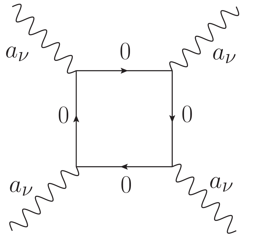
$$+{\sum\limits_{i=1,2}}\,{\sum\limits_{j=1,2}}\,{\sum\limits_{n\neq 0}}$$

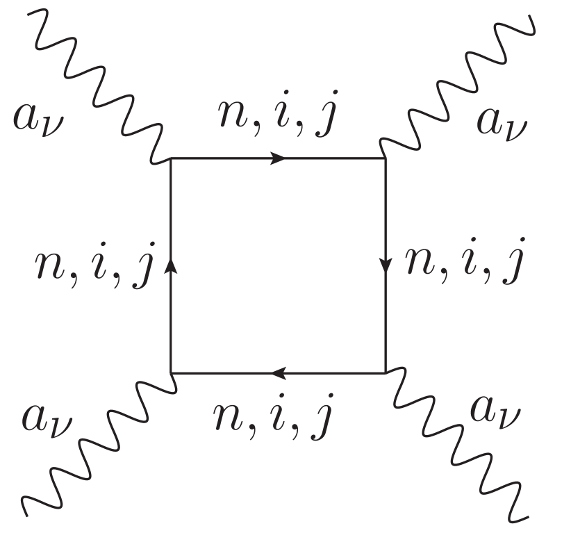
Figure 1: Schematic representation of the elastic $\gamma\gamma$ scattering amplitude. The number near the fermionic line corresponds to the number of the massive fermionic mode which is represented by this line.

In principle, in accordance with action (71), an inelastic $\gamma\gamma$ scattering with massive vector bosons in final states is also possible. However, below we will consider the case when the energy of the initial photon in the c.m. frame is much smaller than $\frac{m}{\sqrt{2}}$, in this case the creation of massive vector bosons is kinematically forbidden. The amplitude of the process presented in Figure 1 can be easily calculated using the known results obtained in QED, see, for example, [18]. For $\omega\ll\mu_{0}=M$, where $\omega$ is the energy of the photon in the c.m. frame, the renormalized contribution of each mode to the amplitude in the leading order in $\frac{\omega}{\mu_{n}}$ is given by

$$A_{n}=\frac{\omega^{4}}{\mu_{n}^{4}}F(\theta),$$ (72)

where the function $F(\theta)$ depends on the scattering angle $\theta$ and the polarizations of the photons, $n=0$ corresponds to the zero localized mode with $\mu_{0}=M$. The explicit form of $F(\theta)$ will be irrelevant for our analysis, but it can be found, for example, in [18]. Thus, we get

$$A=A_{0}+4\sum\limits_{n=1}^{N+1}A_{n}=\left(\frac{\omega^{4}}{\mu_{0}^{4}}+4\sum\limits_{n=1}^{N+1}\frac{\omega^{4}}{\mu_{n}^{4}}\right)F(\theta).$$ (73)

It is easy to show that this amplitude diverges in the limit $\Delta\mu\to 0$. Indeed,

$$A = \left(\frac{\omega^{4}}{\mu_{0}^{4}}+4\sum\limits_{n=1}^{N+1}\frac{\omega^{4}}{\mu_{n}^{4}}\right)F(\theta)>4\sum\limits_{n=1}^{N+1}\frac{\omega^{4}}{\mu_{N+1}^{4}}F(\theta)=4(N+1)\frac{\omega^{4}}{\mu_{N+1}^{4}}F(\theta)=$$

$$= 4\frac{\omega^{4}}{{\tilde{M}}^{4}}\left(1+\frac{\tilde{M}-\sqrt{\frac{m^{2}}{2}+M^{2}}}{\Delta\mu}\right)F(\theta)\underset{\Delta\mu\to 0}{\longrightarrow}\infty,$$

leading to an infinite cross-section, even with the finite cut-off scale $\tilde{M}$, which, of course, contradicts the experimental data and predictions of the Standard Model. This infinity is not the same as the infinities, which arise in QED and which can be removed by applying the standard renormalization procedure, the same growth of the amplitude would appear if we begun to add extra ”electrons” into the standard QED. Technically this happens because the coupling constant of each fermion to the photon remains finite in the limit $N\to\infty$. This differs from the case of brane world models discussed in [19], where there is a single fermion in four-dimensional effective theory and a continuous spectrum of massive vector modes, which couple to this fermion (such a coupling is absent in the model discussed in this paper because of our choice of the parameters). The interaction term of the model discussed in [19] has the form

$$\int dm\Psi(m)\int d^{4}xB_{\mu}(x,m)\bar{\psi}\gamma^{\mu}\psi.$$ (75)

After the discretization (with the redefinition of the field $\sqrt{\Delta m}B_{\mu}(x,m_{n})\to B_{\mu}^{n}(x)$) we arrive at

$$\sum\limits_{n}\sqrt{\Delta m}\Psi_{n}\int d^{4}xB_{\mu}^{n}(x)\bar{\psi}\gamma^{\mu}\psi.$$ (76)

We see that in the model [19] the coupling constant tends to zero in the limit $\Delta m\to 0$. Thus, the decreasing coupling constants and increasing number of the modes compensate each other and one gets a finite result in such a case, contrary to the case of the model discussed in this paper.

Finally it should be noted that one can not obtain an analogous result by taking, say, five-dimensional electrodynamics and considering the scattering of five-dimensional photons with $p_{4}=0$ holding for in- and out- photons, where $p_{4}$ is the photon momentum in the extra coordinate in the c.m. frame. Let us show it very schematically. The wave function of the photon in the extra dimension in the case $p_{4}=0$ does not depend on $x^{4}$, and integration over $x^{4}$ in the free photon action will lead to an infinite value. Of course, this infinite value can be incorporated into the photon field proper by making the corresponding redefinition of this field, just by putting the theory into the box of length $L$ in the extra dimension and then redefining the field as $\sqrt{L}A_{\mu}\to A_{\mu}$. Formally the effective action in this case appears to be analogous to the one presented above (of course, without a mass gap etc.) The coupling constant in this case appears to be redefined as $e_{new}=e/\sqrt{L}$, which tends to zero at $L\to\infty$. In order to have the coupling constant $e_{new}$ be finite in the limit $L\to\infty$, which is exactly the case described by (64), one should suppose that the initial coupling constant in five-dimensional electrodynamics is infinite. Thus, our effective theory described by action (64) is similar in some sense to five-dimensional electrodynamics with an infinite coupling constant.

5 Passing from continuous to discrete spectrum – does it help?

In the previous section it was shown that the existence of a continuous spectrum causes a problem in the low-energy effective theory. Moreover, it looks as if such a problem is inherent to all multidimensional models providing a continuous spectrum of excited fermionic modes which have finite coupling constants to an isolated vector zero mode. Of course, the simplest solution is just to suppose that the cut-off scale $\tilde{M}$ is smaller than $\sqrt{M^{2}+\frac{h^{2}}{\lambda}m^{2}}\approx\frac{hm}{\sqrt{\lambda}}$ for $M\ll\frac{hm}{\sqrt{\lambda}}$. But $\frac{hm}{\sqrt{\lambda}}$ is exactly the factor which defines the inverse width of the wave function of the zero fermionic mode, see (2). Thus, the cut-off scale should be much larger than $\frac{hm}{\sqrt{\lambda}}$, otherwise it appears to be very unrealistic and rather strange to consider the cut-off scale to be smaller than one of the typical scales of the effective theory we are using to construct the model.

Another possible solution to the problem is to replace the continuous spectrum by a completely discrete spectrum. This can be done by changing the form of the interaction of five-dimensional fermions with the background scalar field. Indeed, let us consider the following form of the interaction term:

$$h\,\textrm{arctanh}\left({\frac{\sqrt{\lambda}}{m}\Phi}\right)\left(\bar{\Psi}_{2}\Psi_{2}-\bar{\Psi}_{1}\Psi_{1}\right)$$ (77)

instead of

$$h\Phi\left(\bar{\Psi}_{2}\Psi_{2}-\bar{\Psi}_{1}\Psi_{1}\right).$$ (78)

Of course, this term looks very artificial and unnatural, but note that this is just a toy model. The equation of motion for the wave function $f(z)$ (analogous to eq. (30)) in this case and with (1) takes the form

$$\left(\mu^{2}-M^{2}+\frac{hm}{\sqrt{2}}\right)f(z)=-f^{\prime\prime}(z)+\frac{h^{2}m^{2}}{2}z^{2}f(z).$$ (79)

This is the standard quantum mechanical equation for the harmonic oscillator. According to the fact that solutions to this equation should be normalizable (see (35)), we get the well-known spectrum

$$\mu_{n}^{2}=M^{2}+hm\sqrt{2}n,\qquad n=0,1,...,\infty.$$ (80)

It is evident that there is no continuous spectrum in this case. The wave function of the zero mode takes the form

$$f(z)\sim e^{-\frac{hm}{2\sqrt{2}}z^{2}},\qquad{\tilde{f}}(z)\equiv 0.$$ (81)

We see that this wave function decreases much faster with $z\to\infty$ in comparison with (2). As for amplitude (73), in this case it takes the form

$$A=\frac{\omega^{4}}{\mu_{0}^{4}}F(\theta)+2\sum\limits_{n=1}^{\infty}\frac{\omega^{4}}{\mu_{n}^{4}}F(\theta)\approx\omega^{4}\left(\frac{1}{M^{4}}+\frac{\pi^{2}}{6h^{2}m^{2}}\right)F(\theta)$$ (82)

for $hm\gg M^{2}$, it is finite and the contribution of the excited modes appears to be highly suppressed for $hm\gg M^{2}$.

The existence of the continuous spectrum of the vector modes seems to be not so dangerous, see small discussion on this topic in the previous section. Nevertheless, one can also replace the continuous spectrum by a discrete spectrum by considering a Lagrangian of the (again very artificial) form

$$S=-\int\xi^{2}\exp{\left(-\beta^{2}\textrm{arctanh}^{2}\left({\frac{\sqrt{\lambda}}{m}\Phi}\right)\right)}\frac{1}{4}F^{MN}F_{MN}d^{4}xdz.$$ (83)

It is very easy to show that in this case and with (1) we again get the equation for the harmonic oscillator instead of (55) (the weight function $\sim e^{-c^{2}z^{2}}$ for a vector field, leading to such an equation for the wave functions of its modes, was discussed in [7]), moreover, by adjusting $\beta$ we can get the equation with the same r.h.s. as that in (79). In such a fine-tuned case again there are no terms describing the interaction of two zero-mode fields with one excited mode in the effective four-dimensional Lagrangian. If the masses of the excited states are large, they will not affect the four-dimensional low-energy effective theory. It is interesting to note that such a mechanisms of localization in principle can simulate a compact extra dimension: from the four-dimensional point of view such a theory can be treated as a five-dimensional theory with a compact extra dimension, and the corresponding localized modes – as the Kaluza-Klein modes arising from a compact extra dimension.

Nevertheless, this is not the whole story. There is another continuous spectrum in the theory under consideration – the spectrum of the scalar fluctuations above the kink solution. Since these modes couple both to the vector bosons and to the fermions, one can expect divergencies, analogous to those discussed earlier, resulting from the contribution of the scalar modes from the continuous spectrum of the fluctuations above the background kink solution. For example, in the case of interaction (57) the scalar fluctuations couple quadratically to the vector field (through the term in front of the kinetic term in (57)), and there arises an interaction term of the form

$$\frac{\lambda}{2^{\frac{3}{2}}m}\int\limits_{\sqrt{2}m}^{\infty}d\mu\int\varphi_{(\mu)}^{2}f^{\rho\nu}f_{\rho\nu}d^{4}x,$$ (84)

where $\varphi_{(\mu)}$ are the fluctuations above the kink solution. Such an interaction again can give an infinite contribution to the elastic $\gamma\gamma$ scattering amplitude. Note that one should not expect a compensation of divergencies produced by the fermionic modes and the scalar modes as it happens in SUSY theories – the coupling constant of the scalar modes does not include the electric charge $e$, see (84). Indeed, there is no extra symmetry which could provide such a compensation. It is very probable that an analogous problem arises in the case of (77) and (83), because there are quadratic in $\varphi_{(\mu)}$ and higher power terms in the expansion of (83) in terms of $\varphi_{(\mu)}$.

6 Conclusion

In this paper we discussed a model, describing a localization of fermions and gauge bosons on a domain wall. It is shown that the mechanism of localization of gauge fields, which is based on the ideas proposed in [6, 7, 8], provides a constant wave function of the zero mode in the extra dimension and ensures the universality of charge. The latter is crucial for localizing non-abelian gauge fields and constructing realistic models of fields localization. We also discussed the mechanism of fermion localization, based on the well-known Rubakov-Shaposhnikov mechanism [1], which allows one to get four-dimensional massive fermions localized on a domain wall. All the key ingredients of this mechanism were presented in the literature earlier, see [9, 10, 12, 13], but we examined its main properties in the case of localization on a domain wall and found some very interesting consequences.

Both mechanisms of localization provide nonzero mass gaps between the lowest zero and the subsequent modes. This allows us to construct a simple five-dimensional model, resulting in an effective four-dimensional theory, whose zero-mode sector represents ordinary spinor electrodynamics localized on a domain wall of the standard kink profile. But it appears that the model possesses a very peculiar property – it leads to an infinite (renormalized) amplitude of $\gamma\gamma\to\gamma\gamma$ scattering process, which is known to be finite in ordinary four-dimensional QED. A possible solution to this problem could be in considering other forms of interaction of the background scalar field with matter fields, which could lead to discrete spectra of the excited modes of matter fields instead of the continuous spectra. But most probably the existence of the continuous spectrum of the fluctuations above the kink background solution again would lead to unremovable divergencies in the amplitudes and the cross-sections. Thus, there arises a question about more realistic mechanisms of matter fields localization on a domain wall.

Appendix

The interaction term, describing the coupling of the massive fermions and vector bosons to the zero mode fermion can be obtained by substituting (61)-(63) into (60) and has the form

$$\frac{e\sqrt{\lambda}}{2^{\frac{3}{4}}\sqrt{m}}\sum\limits_{j,j^{\prime}=1}^{2}\int dz\int\limits_{\frac{m}{\sqrt{2}}}^{\infty}d\mu_{1}\int\limits_{\sqrt{\frac{m^{2}}{2}+M^{2}}}^{\infty}d\mu\,y_{(\mu_{1},j^{\prime})}(z)f_{(\mu,j)}(z)J^{\nu}_{(\mu,j)}a_{\nu}^{(\mu_{1},j^{\prime})}=\frac{e\sqrt{\lambda}}{2^{\frac{3}{4}}\sqrt{m}}\times$$

$$\times\sum\limits_{j,j^{\prime}=1}^{2}\int dz\int\limits_{\sqrt{\frac{m^{2}}{2}+M^{2}}}^{\infty}\frac{\mu^{\prime}d\mu^{\prime}}{\sqrt{{\mu^{\prime}}^{2}-M^{2}}}\int\limits_{\sqrt{\frac{m^{2}}{2}+M^{2}}}^{\infty}d\mu\,y_{(\sqrt{{\mu^{\prime}}^{2}-M^{2}},j^{\prime})}(z)f_{(\mu,j)}(z)J^{\nu}_{(\mu,j)}a_{\nu}^{(\sqrt{{\mu^{\prime}}^{2}-M^{2}},j^{\prime})}.$$

where $J^{\nu}_{(\mu,j)}=\bar{\psi}^{(\mu,j)}_{s}\gamma^{\nu}\psi+\bar{\psi}\gamma^{\nu}\psi^{(\mu,j)}_{s}$. It is evident from (30) (with $\frac{h}{\sqrt{\lambda}}=\frac{1}{\sqrt{2}}$) and (55) that $f_{(\mu,j)}(z)=C_{f}^{(\mu)}y_{(\sqrt{{\mu}^{2}-M^{2}},j)}(z)$. The constant $C_{f}^{(\mu)}$ simply reflects the fact that the wave functions $y_{(\mu^{\prime},j)}(z)$ and $f_{(\mu,j)}(z)$ possess different normalization conditions. In general, one can calculate $C_{f}^{(\mu)}$ using the exact forms of $y_{(\mu^{\prime},j)}(z)$ and $f_{(\mu,j)}(z)$ (for the case $\frac{h}{\sqrt{\lambda}}=\frac{1}{\sqrt{2}}$ the wave functions $\tilde{f}_{(\mu,1)}(z)=c\sin\left(\sqrt{{\mu}^{2}-M^{2}-\frac{m^{2}}{2}}\,z\right)$, $\tilde{f}_{(\mu,2)}(z)=c\cos\left(\sqrt{{\mu}^{2}-M^{2}-\frac{m^{2}}{2}}\,z\right)$ and explicit form of the function $f_{(\mu,j)}(z)$ (and of the function $y_{(\mu^{\prime},j)}(z)$ also) can be obtained with the help of (23)).

Thus, we get

$$\frac{e\sqrt{\lambda}}{2^{\frac{3}{4}}\sqrt{m}}\sum\limits_{j,j^{\prime}=1}^{2}\int dz\int\limits_{\sqrt{\frac{m^{2}}{2}+M^{2}}}^{\infty}\frac{\mu^{\prime}d\mu^{\prime}}{\sqrt{{\mu^{\prime}}^{2}-M^{2}}}\int\limits_{\sqrt{\frac{m^{2}}{2}+M^{2}}}^{\infty}d\mu\,y_{(\sqrt{{\mu^{\prime}}^{2}-M^{2}},j^{\prime})}(z)C_{f}^{(\mu)}y_{(\sqrt{{\mu}^{2}-M^{2}},j)}(z)\times$$

$$\times J^{\nu}_{(\mu,j)}a_{\nu}^{(\sqrt{{\mu^{\prime}}^{2}-M^{2}},j^{\prime})}=$$

$$=\frac{e\sqrt{\lambda}}{2^{\frac{3}{4}}\sqrt{m}\xi^{2}}\sum\limits_{j=1}^{2}\int\limits_{\sqrt{\frac{m^{2}}{2}+M^{2}}}^{\infty}\frac{\mu^{\prime}d\mu^{\prime}}{\sqrt{{\mu^{\prime}}^{2}-M^{2}}}\int\limits_{\sqrt{\frac{m^{2}}{2}+M^{2}}}^{\infty}d\mu\,\delta\left(\sqrt{{\mu^{\prime}}^{2}-M^{2}}-\sqrt{{\mu}^{2}-M^{2}}\right)\times$$

$$\times C_{f}^{(\mu)}J^{\nu}_{(\mu,j)}a_{\nu}^{(\sqrt{{\mu^{\prime}}^{2}-M^{2}},j)}=\frac{e\sqrt{\lambda}}{2^{\frac{3}{4}}\sqrt{m}\xi^{2}}\sum\limits_{j=1}^{2}\int\limits_{\sqrt{\frac{m^{2}}{2}+M^{2}}}^{\infty}d\mu\,C_{f}^{(\mu)}J^{\nu}_{(\mu,j)}a_{\nu}^{(\sqrt{{\mu}^{2}-M^{2}},j)}$$

and $C_{\psi,a}^{(\mu)}=\frac{e\sqrt{\lambda}}{2^{\frac{3}{4}}\sqrt{m}\xi^{2}}C_{f}^{(\mu)}=\frac{e_{4}}{\xi}C_{f}^{(\mu)}$.

References

• [1] V.A. Rubakov and M.E. Shaposhnikov, Phys. Lett.  B 125 (1983) 136.
• [2] G.R. Dvali and M.A. Shifman, Phys. Lett. B 396 (1997) 64 [Erratum-ibid. B 407 (1997) 452].
• [3] S.L. Dubovsky and V.A. Rubakov, Int. J. Mod. Phys.  A 16 (2001) 4331.
• [4] V.A. Rubakov, Phys. Usp. 44 (2001) 871.
• [5] S.L. Dubovsky, V.A. Rubakov and P.G. Tinyakov, JHEP 0008 (2000) 041.
• [6] A. Kehagias and K. Tamvakis, Phys. Lett.  B 504 (2001) 38.
• [7] M.E. Shaposhnikov and P. Tinyakov, Phys. Lett.  B 515 (2001) 442.
• [8] A.T. Barnaveli and O.V. Kancheli, Sov. J. Nucl. Phys.  52 (1990) 576.
• [9] S.L. Dubovsky, V.A. Rubakov and P.G. Tinyakov, Phys. Rev.  D 62 (2000) 105011.
• [10] M.V. Libanov and S.V. Troitsky, Nucl. Phys.  B 599 (2001) 319.
• [11] R. Casadio and A. Gruppuso, Phys. Rev.  D 64 (2001) 025020.
• [12] A.A. Andrianov, V.A. Andrianov, P. Giacconi and R. Soldati, JHEP 0307 (2003) 063.
• [13] A.A. Andrianov, V.A. Andrianov, P. Giacconi and R. Soldati, JHEP 0507 (2005) 003.
• [14] A.E.R. Chumbes, J.M. Hoff da Silva and M.B. Hott, arXiv:1108.3821 [hep-th].
• [15] S. Flügge, Practical Quantum Mechanics – Volume 1 and Volume 2, 1971 (Springer).
• [16] C. Macesanu, Int. J. Mod. Phys. A 21 (2006) 2259.
• [17] A.T. Barnaveli and O.V. Kancheli, Sov. J. Nucl. Phys.  51 (1990) 573.
• [18] A.I. Ahiezer, V.B. Beresteckiy, Quantum Electrodynamics, 1981 (Nauka, Moscow).
• [19] D.I. Astakhov, D.V. Kirpichnikov, Phys. Rev.  D83 (2011) 104031.
• [20] D. Binosi, L. Theussl, Comput. Phys. Commun.  161 (2004) 76.
D. Binosi, J. Collins, C. Kaufhold, L. Theussl, Comput. Phys. Commun.  180 (2009) 1709.