HPQCD collaboration

Fast Fits for Lattice QCD Correlators

Abstract

We illustrate a technique for fitting lattice QCD correlators to sums of exponentials that is significantly faster than traditional fitting methods — 10–40 times faster for the realistic examples we present. Our examples are drawn from a recent analysis of the $\Upsilon$ spectrum, and another recent analysis of the $D\!\to\!\pi$ semileptonic form factor. For single correlators, we show how to simplify traditional effective-mass analyses.

Most physics results in lattice QCD come from fits of lattice correlators to sums of exponentials. For example, we study a particular hadron by computing Monte Carlo simulation estimates $G_{ab}^{\mathrm{MC}}(t)$ of hadronic correlators,

$$\sum_{\mathbf{x}}\langle 0|\Gamma_{b}(\mathbf{x},t)\Gamma_{a}(0,0)|0\rangle,$$ (1)

with different sources $\Gamma_{a}$ and sinks $\Gamma_{b}$ that create and destroy the hadron. The sum over all spatial sites $\mathbf{x}$ restricts the hadrons to states with zero total three-momentum. Such a correlator can be decomposed into contributions from energy eigenstates $|E_{j}\rangle$ in QCD bib-sumexp :

$$G_{ab}(t;N)=\sum_{j=1}^{N}a_{j}b_{j}\exp(-E_{j}t)$$ (2)

where $E_{j}$ is the energy, with $E_{j}\!\geq\!E_{j-1}$, and the amplitudes are matrix elements, with

$$a_{j}^{*} =\langle 0|\Gamma_{a}(0,0)|E_{j}\rangle,$$

$$b_{j} =\langle 0|\Gamma_{b}(0,0)|E_{j}\rangle.$$ (3)

The physics is in the energies and the matrix elements, and these are determined by fitting fomula (2) to the Monte Carlo data $G_{ab}^{\mathrm{MC}}(t)$ for a variety of sources and sinks.

In principle, the number of terms $N$ in Eq. (2) is infinite, but, in practice, we need only retain a finite number of terms because the exponentials suppress high-energy states. The number needed depends upon the precision of the simulation data $G_{ab}^{\mathrm{MC}}$, but it is not uncommon to require $N\!=\!10$ or more terms for good fits to accurate data. The fitting process becomes both cumbersome and time consuming if many correlators must be fit simultaneously while using such large $N$s. In this paper we introduce a method that can dramatically simplify and accelerate such fits.

The key to this new approach lies in how priors are introduced. Two types of input data are required for these fits. The first is simulation data for the correlators, consisting of Monte Carlo averages $\overline{G}$ for each $a$, $b$ and $t$, and a covariance matrix $\sigma^{2}$ that specifies both the statistical uncertainties in each average and the correlations between them:

$$G_{ab}^{\mathrm{MC}}(t)\leftrightarrow\left\{\overline{G}_{ab}(t),\sigma^{2}_{ab,a^{\prime}b^{\prime}}(t,t^{\prime})\right\}$$ (4)

This data contributes

$$\chi^{2}_{\mathrm{MC}}(a_{j}, b_{j},E_{j})=\sum_{t,a,b}\sum_{t^{\prime},a^{\prime},b^{\prime}}\left(G_{ab}(t;N)-\overline{G}_{ab}(t)\right)$$

$$\sigma^{-2}_{ab,a^{\prime}b^{\prime}}(t,t^{\prime})\left(G_{a^{\prime}b^{\prime}}(t^{\prime};N)-\overline{G}_{a^{\prime}b^{\prime}}(t^{\prime})\right)$$ (5)

to the $\chi^{2}$ function that is minimized by varying parameters $a_{j}$, $b_{j}$, and $E_{j}$ in a conventional fit.

The second type of input data consists of Bayesian priors for each fit parameter. Complicated multi-correlator, multi-parameter fits are impossible without a priori estimates for each fit parameter Lepage:2001ym :

$$a^{\mathrm{pr}}_{j} \equiv\overline{a}_{j}\pm\sigma_{a_{j}},$$

$$b^{\mathrm{pr}}_{j} \equiv\overline{b}_{j}\pm\sigma_{b_{j}},$$

$$E^{\mathrm{pr}}_{j} \equiv\overline{E}_{j}\pm\sigma_{E_{j}}.$$ (6)

This information is included in a conventional fit by adding extra terms to $\chi^{2}(a_{j},b_{j},E_{j})$: $\chi^{2}\!=\!\chi^{2}_{\mathrm{MC}}+\chi^{2}_{\mathrm{pr}}$ where

$$\chi^{2}_{\mathrm{pr}} (a_{j},b_{j},E_{j})=$$

$$\sum_{j=1}^{N}\left\{\frac{(a_{j}-\overline{a}_{j})^{2}}{\sigma_{a_{j}}^{2}}+\frac{(b_{j}-\overline{b}_{j})^{2}}{\sigma_{b_{j}}^{2}}+\frac{(E_{j}-\overline{E}_{j})^{2}}{\sigma_{E_{j}}^{2}}\right\}.$$ (7)

The priors can also be combined to give a priori estimates for the correlators,

$$G_{ab}^{\mathrm{pr}}(t;N)\equiv\sum_{j=1}^{N}a_{j}^{\mathrm{pr}}b_{j}^{\mathrm{pr}}\exp(-E_{j}^{\mathrm{pr}}t),$$ (8)

where the means and covariance matrix for $G_{ab}^{\mathrm{pr}}(t)$ are computed, using standard error propagation, from the means and covariance matrix of the priors (Eq. (6)).

The cost of a traditional analysis goes up rapidly with the number of parameters needed to obtain a good fit. In practice, however, we are rarely interested in parameters from the large-$j$ terms in fit function (2), even when these terms are needed for a good fit. Rather than including them in the fit, we can incorporate the large-$j$ terms into the Monte Carlo data before fitting. To do this, we use the priors to generate an a priori estimate for these terms, and then subtract that estimate from the Monte Carlo data. This effectively removes the large-$j$ terms from the data. Finally we fit the modified data with a simpler formula that includes only small-$j$ terms.

More explicitly, we can remove terms having $n\!<\!j\!\leq\!N$ by replacing $G^{\mathrm{MC}}_{ab}(t)$ with (first definition)

$${\tilde{G}}_{ab}^{\mathrm{MC}}(t;n)\equiv G_{ab}^{\mathrm{MC}}(t)-\Delta G_{ab}^{\mathrm{pr}}(t;n),$$ (9)

where

$$\Delta G^{\mathrm{pr}}_{ab}(t;n) \equiv G_{ab}^{\mathrm{pr}}(t;N)-G_{ab}^{\mathrm{pr}}(t;n)$$

$$=\sum_{j=n+1}^{N}a_{j}^{\mathrm{pr}}b_{j}^{\mathrm{pr}}\exp(-E_{j}^{\mathrm{pr}}t)$$ (10)

is the $j\!>\!n$ part of the fit function. Having removed the $j\!>\!n$ terms, we can fit $\tilde{G}_{ab}^{\mathrm{MC}}(t;n)$ with the simpler fit function, $G_{ab}(t;n)$, rather than $G_{ab}(t;N)$.

Here we assume that $N$ is sufficiently large that $\Delta G_{ab}^{\mathrm{pr}}(t;n)$ and therefore $\tilde{G}_{ab}^{\mathrm{MC}}(t;n)$ are independent of $N$ to within their statistical errors. The covariance matrix for $\tilde{G}_{ab}^{\mathrm{MC}}(t;n)$ is obtained by adding the covariance matrices of $G_{ab}^{\mathrm{MC}}(t)$ and $\Delta G_{ab}^{\mathrm{pr}}(t;n)$ (that is, adding the errors in quadrature) bib-errors .

Removing high-$j$ terms from both the fit function and the fit data replaces the original fitting problem — fit an $N$-term function $G_{ab}(t;N)$ to $G_{ab}^{\mathrm{MC}}(t)$ — by a simpler problem that can have far fewer fit parameters: fit an $n$-term function $G_{ab}(t;n)$ to ${\tilde{G}}_{ab}^{\mathrm{MC}}(t;n)$, where $n\!<\!N$. Remarkably, as we showed in McNeile:2010ji , these two problems are equivalent for high statistics data even when $n$ is quite small: that is, fit results (means and standard deviations) for the low-$j$ parameters are the same in both cases. In the second case, the $j\!>\!n$ terms have been “marginalized,” or, in effect, integrated out of the Bayesian probability distribution, but in a way that does not affect the analysis of the $j\!\leq\!n$ terms. When $n\!\ll\!N$, the fit parameters that remain are many fewer than what would be required in a standard fit, and fitting is much faster.

In this paper we use a variation of this marginalization procedure which we find to be more robust when fitting correlators that fall exponentially quickly with increasing $t$. In this variation the modified correlators are given by (second definition)

$$\tilde{G}_{ab}^{\mathrm{MC}}(t;n)\equiv G_{ab}^{\mathrm{MC}}(t)\,\frac{G_{ab}^{\mathrm{pr}}(t;n)}{G_{ab}^{\mathrm{pr}}(t;N)},$$ (11)

which is analogous to the first definition (Eq. (9)) but applied to the logarithm of the correlator rather than the correlator itself. Again, terms with $j\!>\!n$ have been removed, and therefore the modified correlator data can be fit with the simpler fit function, $G_{ab}(t;n)$.

Figure 1: Fit $\chi^{2}$ per degree of freedom for sequential fits of 25 $\Upsilon$ correlators with $n\!=\!1,2,3\ldots$ terms in fit function (2). Results are plotted versus the cumulative time required for fitting, and are for fits of: a) the unmodified simulation data $G_{ab}^{\mathrm{MC}}(t)$ (red circles and dotted line); and b) the modified simulation data $\tilde{G}_{ab}^{\mathrm{MC}}(t;n)$ (Eq. (11)) (blue circles and dashed line). The region of good fits is indicated by the gray band.

We now illustrate our new method by applying it to QCD simulation data from two recent analyses. For each analysis, we fit a function, like $G_{ab}(t;n)$, with $n$ terms both to untouched simulation data $G_{ab}^{\mathrm{MC}}(t)$, and to modified simulation data $\tilde{G}_{ab}^{\mathrm{MC}}(t;n)$, from which $j\!>\!n$ terms have been removed using Eq. (11). We vary $n$, doing sequential fits with $n\!=\!1,2,3\ldots$, where the best-fit parameter values from one fit are used as starting values for the next fit. Sequential fitting with increasing $n$ is a standard approach to complicated multi-parameter correlator fits; $n$ is increased until the fit’s $\chi^{2}$ stops changing, at which point enough terms have been include to reflect accurately the uncertainties introduced by large-$j$ terms. Here we examine the best-fit parameters for each $n$ to investigate the rate at which correct results emerge from this process. This allows a detailed comparison of our two fitting strategies.

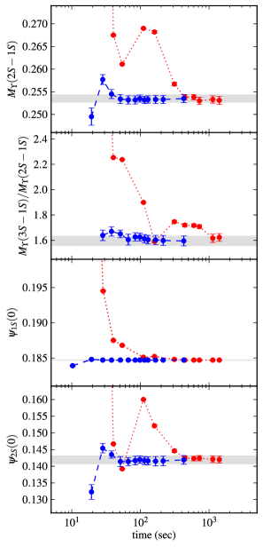
Figure 2: Best-fit results from sequential fits of 25 $\Upsilon$ correlators with $n\!=\!1,2,3\ldots$ terms in fit function (2). Results are plotted versus the cumulative time required for fitting, and are for fits of: a) the unmodified simulation data $G_{ab}^{\mathrm{MC}}(t)$ (red circles and dotted line); and b) the modified simulation data $\tilde{G}_{ab}^{\mathrm{MC}}(t;n)$ (Eq. (11)) (blue circles and dashed line). Results are given for mass splittings between different vector $S$-states, and for the wave functions at the origin for the lowest two states. All results are in lattice units. The gray bands show the best-fit result from the modified data after convergence.

The first data set is a collection of 25 correlators for the $\Upsilon(1S)$ meson and its radial excitations ($\Upsilon(2S)$, $\Upsilon(3S)$, etc.) ups-paper . These correlators were made using five different operators for both sources and sinks. They were fit to formula (2) with priors (in lattice units):

$$\log(E_{1}) =\log(0.3\pm 0.1)=-1.2\pm 0.3$$

$$\log(E_{j+1}-E_{j}) =\log(0.25\pm 0.125)=-1.4\pm 0.5$$

$$a_{j} =0.1\pm 1.0$$ (12)

except for a local source for which the priors were $\log(a_{j})\!=\!\log(0.1\pm 0.2)\!=\!-2.3\pm 2$ (local source). These are broad priors — more than 100 times broader than the final errors for the quantities we examine below. We set $N\!=20$ when defining $\tilde{G}_{ab}^{\mathrm{MC}}(t;n)$ (Eq. (11)); this is roughly twice the size it needs to be, but it costs little to make $N$ large. In general $N$ should be chosen so that terms with $j\!>\!N$ are negligible compared with statistical errors.

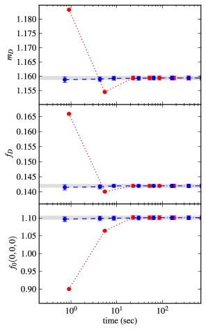
Figure 3: Best-fit results from sequential fits of 13 two-point and three-point correlators for $D$ and $\pi$ mesons with $n\!=\!1,2,3\ldots$ terms in fit function (2). Results are plotted versus the cumulative time required for fitting, and are for fits of: a) the unmodified simulation data (red circles and dotted line); and b) the modified simulation data (Eq. (11)) (blue circles and dashed line). Results are given for the $D$-meson mass $m_{D}$ and decay constant $f_{D}$, and for the $D\!\to\!\pi$ scalar form factor at zero recoil momentum $f_{0}(0,0,0)$. All results are in lattice units. The gray bands show the best-fit result from the modified data after convergence.

In Fig. 1 we plot the $\chi^{2}$ per degree of freedom for each method versus the time required to get to that value ref-time . As expected, the new algorithm reaches a reasonable $\chi^{2}$ with just a few terms ($n\!=\!2$–3), in 20–30 seconds; the traditional algorithm requires $n\!=\!10$–11 to obtain a good $\chi^{2}$, and 600–700 seconds. Similar differences are evident if we look at physical quantities extracted from the simulations. In Fig. 2 we show results for the $2S-1S$ mass splitting (in lattice units), for the $3S-1S$ mass splitting divided by the $2S-1S$ splitting, and for the $1S$ and $2S$ mesons’ (nonrelativistic) wave functions at the origin, which come from fit parameters $a_{j}$ for a local source. In every case the two algorithms agree on the final result, but the new algorithm converges to correct results 10–40 times faster.

Our second example is from a recent analysis of the $D\!\to\!\pi$ semileptonic form factor Na:2011mc . To extract the form factor at four different momenta, this analysis uses a simultaneous fit of 13 two-point and three-point correlators: a) a $D$-meson correlator with a pseudoscalar local source and sink; b) four $\pi$-meson correlators, one for each pion momentum of interest, again with local pseudoscalar sources and sinks; and c) two three-point correlators $D\!\to\!J_{\mathrm{scalar}}\!\to\!\pi$ for each of the four pion momenta. The fit functions are more complicated for this case. For example, the $D$-meson correlator is fit by a function:

$$G_{D}(t;n)=\sum_{j=1}^{n}a_{j}\,f(E_{j},t)-(-1)^{t}a_{j}^{o}\,f(E^{o}_{j},t)$$ (13)

where $f(E_{j},t)\!\equiv\!\exp(-E_{j}t)+\exp(-E_{j}(T-t))$ is periodic with period $T\!=\!64$, and the second (oscillating) term is due to opposite-parity states in the correlator (a feature of staggered-quark formalisms like that used in this analysis). The details for the other correlators, and the priors are given in Na:2011mc .

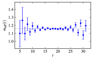
Figure 4: The $D$-meson’s effective mass $m_{\mathrm{eff}}(t)$ versus $t$ computed from modified simulation data $\tilde{G}_{D}^{\mathrm{MC}}(t)$ from which every state other than the ground state has been removed (using priors). The (very thin) gray band shows the weighted average of all $m_{\mathrm{eff}}(t)$s, taking account of correlations. The thickness of the band indicates the uncertainty of the average. Note that the largest $t$s shown here correspond to the middle $t$ range. The error bars grow there because $m_{\mathrm{eff}}(t)$ becomes very sensitive to statistical errors in this region (since periodic boundary conditions imply that the derivative of the correlator’s non-oscillating part vanishes at the midpoint).

Despite the complexity of dealing with both two-point and three-point correlators, this is a simpler fit than the $\Upsilon$ case; but even here we find that marginalizing most of the fit function makes the analysis about 30 times faster. We show results in Fig. 3 for the $D$-meson’s mass $m_{D}$ and leptonic decay constant $f_{D}$, as well as for the $D\!\to\!\pi$ scalar form factor $f_{0}(0,0,0)$ at zero recoil momentum. All results are in lattice units. Again the two approaches agree on the results but the new approach has correct results even with only a single term ($n\!=\!1$) in the fit functions. For these fits we set $N\!=\!10$ when computing the modified data $\tilde{G}_{ab}^{\mathrm{MC}}(t;n)$ (Eq. (11)), which is twice as large as it needs to be.

Some insight into how marginalization works can be gained by focusing just on the $D$ correlator from this analysis and fitting the modified data,

$$\tilde{G}_{D}^{\mathrm{MC}}(t)\equiv G_{D}^{\mathrm{MC}}(t)\,\frac{a_{1}^{\mathrm{pr}}f(E_{1}^{\mathrm{pr}},t)}{G_{D}^{\mathrm{pr}}(t;N)},$$ (14)

with only the non-oscillating part of the first term in Eq. (13) — that is, with $a_{1}f(E_{1},t)$. This situation is sufficiently simple that fitting is not required. The $D$ mass, for example, can be obtained by averaging the “effective mass,”

$$m_{\mathrm{eff}}(t)\equiv\mathrm{arccosh}\left(\frac{\tilde{G}_{D}^{\mathrm{MC}}(t+1)+\tilde{G}_{D}^{\mathrm{MC}}(t-1)}{2\,\tilde{G}_{D}^{\mathrm{MC}}(t)}\right),$$ (15)

over all $t$, taking account of correlations between different $t$s. The effective mass is plotted as a function of $t$ in Fig. 4. It is compared with the weighted average of all 27 $m_{\mathrm{eff}}(t)$s (gray band), which at $m_{\mathrm{eff}}^{\mathrm{avg}}\!=\!1.1584(11)$ agrees well with the best result, $1.1593(7)$, from full multi-term fits (top panel in Fig. 3).

The first excited state in the $D$ correlator is the opposite-parity contribution, which accounts for the oscillation in $m_{\mathrm{eff}}(t)$. Strong statistical correlations between different points result in an average $m_{\mathrm{eff}}$ whose error is more than 7 times smaller than the best error from an individual $m_{\mathrm{eff}}(t)$. The errors in $m_{\mathrm{eff}}(t)$ when $t\!\leq\!16$ come almost entirely from marginalized terms absorbed into the fit data using Eq. (14); the original Monte Carlo simulation errors are negligible there.

Absent marginalization, contributions from excited states would limit a traditional effective mass analysis of this data to values with $t\!>\!16$. With marginalization, all $t$s are used, except for a small number at very small $t$ where the fit function is invalid (because of temporal non-locality in the lattice quark action). Using 28 $t$s is possible because we have removed the excited states through Eq. (14). As a result different $m_{\mathrm{eff}}(t)$s agree with each other to within their errors: fitting all 27 values in Fig. 4 to a constant gives an excellent fit, with a $\chi^{2}$ per degree of freedom of 0.6. (The result of the fit is, by definition, the same as the weighted average reported above.)

Our new implementation of effective-mass analyses is simpler and less ambiguous than traditional analyses because we are not limited to large $t$s. More importantly our implementation also allows us to quantify the contribution to the uncertainty in the final $m_{\mathrm{eff}}^{\mathrm{avg}}$ due to the excited states: here the priors for non-oscillating terms in Eq. (13) contribute $0.44\sigma_{m}$, those from oscillating terms contribute $0.07\sigma_{m}$, and the uncertainties in the Monte Carlo data contribute $0.89\sigma_{m}$, where $\sigma_{m}$ is the standard deviation of $m_{\mathrm{eff}}^{\mathrm{avg}}$. Such information is essential for assessing the reliability of the final result, as well as for planning improvements to the analysis.

In this paper we have shown how to accelerate multi-exponential fits to multiple hadronic correlators by removing contributions due to excited states from both the fit function and the simulation data, before fitting. This technique for marginalizing large parts of the fit function greatly reduces the number of fit parameters needed in the realistic examples presented here, and makes fitting 10–40 times faster. Marginalization also simplifies effective-mass analyses, and generalizes easily to analogous multi-state (generalized eigenvalue) methods.

This work was supported by the DOE (DE-FG02-04ER41299, DE-FG02-91ER40690), the NSF (PHY-0757868), and the STFC. We used the Darwin Supercomputer of the Cambridge High Performance Computing Service as part of the DiRAC facility jointly funded by STFC, BIS and the Universities of Cambridge and Glasgow. We also used facilities of the USQCD collaboration funded by the Office of Science of the DOE and at the Ohio Supercomputer Center.

References

- [1] Lattice QCD simulations use Euclidean time and so is replaced by in the exponentials. Also simulations are for finite volumes in space, and therefore all states, including multi-hadron states, have discrete energy eigenvalues.
- [2] G. P. Lepage, B. Clark, C. T. H. Davies, K. Hornbostel, P. B. Mackenzie, C. Morningstar, H. Trottier, Nucl. Phys. Proc. Suppl. 106, 12-20 (2002). [hep-lat/0110175]. The formula for generalizes trivially if there are correlations between the priors for different parameters.
- [3] For a proof, see the appendix of C. McNeile, C. T. H. Davies, E. Follana, K. Hornbostel, G. P. Lepage, Phys. Rev. D82, 034512 (2010). [arXiv:1004.4285 [hep-lat]].
- [4] Again the covariance matrix for is computed using standard error propagation — for example, with and . We have compared this linearized analysis with Monte Carlo evaluations of (from normal distributions for the priors). We find the Monte Carlo results to be both much more expensive and also less robust for correlators that decay exponentially quickly. Note also that it is essential to retain the off-diagonal elements (correlations) in the covariance matrix for ; correlations arise because, for example, the prior data used for a parameter is the same for all values.
- [5] The simulations used 0.09 fm lattices with sea quarks (HISQ discretization), and NRQCD dynamics for the quark. The gluon configurations were provided by the MILC collaboration. For further details see: R. J. Dowdall, et al., [arXiv:1110.6887 [hep-lat]].
- [6] The absolute computer times quoted here are obviously of little relevance since they depend upon specific details of hardware and software. What is relevant is the comparison between methods.
- [7] The simulations used 0.12 fm lattices with light sea quarks (ASQTAD discretization), and HISQ relativistic dynamics for valence quarks. The gluon configurations were provided by the MILC collaboration. For further details see (set C2): H. Na, C. T. H. Davies, E. Follana, J. Koponen, G. P. Lepage, J. Shigemitsu, arXiv:1109.1501 [hep-lat].