Quantum computing with incoherent resources and quantum jumps

Abstract

Spontaneous emission and the inelastic scattering of photons are two natural processes usually associated with decoherence and the reduction in the capacity to process quantum information. Here we show that when suitably detected, these photons are sufficient to build all the fundamental blocks needed to perform quantum computation in the emitting qubits while protecting them from deleterious dissipative effects. We exemplify by showing how to teleport an unknown quantum state and how to efficiently prepare graph states for the implementation of measurement-based quantum computation.

In the traditional circuit model of quantum computation Nielsen and Chuang (2000), a quantum algorithm is implemented by the sequential action of entangling gates and local unitaries followed by a final measurement stage that reveals the result of the computation. An alternative approach is the measurement-based quantum computation (MBQC) Raussendorf and Briegel (2001); Raussendorf et al. (2003) where an initial highly entangled multiqubit graph state is prepared and a succession of adaptive measurements on the individual qubits defines the implementation of a specific algorithm. In both scenarios, quantum computation can be carried out with a basic toolbox of three elements: measurements on the computational basis, single qubit rotations, and specific two-qubit entangling gates.

In both computational models, decoherence Giulini and et al. (1996) poses a major obstacle to practical implementations as the qubits are encoded in systems that are unavoidably coupled to the environment. Emitted and scattered photons are two notable examples of natural processes associated with decoherence in quantum systems. However, when detected, the same photons lead to the observation of quantum jumps Carmichael (1993); Sauter et al. (1986); Nagourney et al. (1986); Gleyzes et al. (2007), which can be used to read information out of the systems and to manipulate them to some extent.

Here we show that when the photons spontaneously emitted and inelastically scattered by the qubits into their surrounding environment are suitably monitored, the three elements of the quantum computing toolbox can be implemented. We also show that the same scheme protects the system as a whole from dissipation while the computation is carried on. We exemplify the scheme by showing how to teleport an unknown quantum state, a protocol that already encompasses all the required elements for any quantum computation. Furthermore, our method efficiently produces graph states useful for the implementation of measurement-based quantum computation Raussendorf and Briegel (2001); Raussendorf et al. (2003).

The first tool to be described is how to measure a qubit in the computational basis what is promptly achieved by monitoring its spontaneous emission (see Fig. 1.1). If a non-degenerate qubit, prepared in a superposition $\alpha|g\rangle+\beta|e\rangle$, is allowed to decay at a rate $\gamma$, then, for times much larger than $T=1/\gamma$, the excited (ground) component of the original state of the qubit becomes correlated with the detection (no-detection) of the spontaneously emitted photon. A detection identifies the output $1$ (related to state $|e\rangle$) and defines a quantum jump in the system that, mathematically, corresponds to applying the lowering operator $\sigma_{-}$ to the state of the qubit. On the other hand, no-detection outputs $0$ and is associated to the so-called no-jump trajectory Carmichael (1993); Sauter et al. (1986); Nagourney et al. (1986); Gleyzes et al. (2007). The monitoring of the spontaneous decay is then equivalent to destructively measuring the state of the qubit in the computational basis where, by destructive, we mean that the measurement informs on the state of the qubit but always drags it into its ground state.

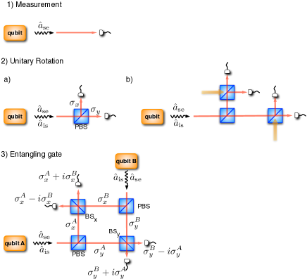
Figure 1: Quantum-jump version of the building blocks for quantum computation. 1) Spontaneous emission (“s.e.”) is sufficient for measuring in the computational basis. 2a) The PBS erases “which process” information and a photon-detection produces a jump proportional to a unitary flip in the emitting qubit. For $\theta=0$ the jumps correspond to $\sigma_{x}$ or $\sigma_{y}$ Carvalho and Santos (2011); at other angles the jumps generate flips ($\pi$ rotations) around other directions in the equator of the Bloch sphere (linear combinations of $\sigma_{x}$ and $\sigma_{y}$). 2b) More general rotations can be obtained through homodyne detection schemes Carvalho and Santos (2011). 3) Entangling gates achieved through a second quantum erasing process: the standard balanced Beam Splitters (BS) erase “which qubit” information and a detection event in one of the available photocounters implements the corresponding maximally entangling operation indicated in the figure. After the first click, the standard BSs are removed and subsequent clicks will simply produce local flips as in (2a).

This “destructive” character means that the remaining tools for quantum computation cannot be obtained solely by monitoring spontaneously emitted (“s.e.”) photons. The curious solution comes from the addition of an extra incoherent process to each qubit: the inelastic scattering (“i.s.”) of photons provided by an external laser field (see Fig. 2-a). When this process optically pumps the emitting system back into its excited state, the detection of photons in the “i.s.” channel implements the complementary “destructive” jump $\sigma_{+}$ on the qubit. However, if both “s.e.” and “i.s.” processes are tuned to output photons that are indistinguishable in frequency and linewidth but of orthogonal circular polarisations, then, by placing polarized beam splitters (PBS) before the photocounters, the “which process” information is erased Scully and Drühl (1982); M. O. Scully (1991). In this case, shown in (Fig.1.2-a), the detection of a photon that comes out of the PBS will implement quantum jumps that are linear combinations of $\sigma_{-}$ and $\sigma_{+}$ corresponding to unitary flips of the type $\cos\theta\sigma_{x}+\sin\theta\sigma_{y}$ on the qubit, with $\theta$ determined by the alignment of the PBS. More general rotations are also possible if these new channels are monitored through homodyne detection Carvalho and Santos (2011) (Fig. 1.2-b) or combined with an external classical photon source.

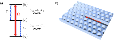
Figure 2: Level scheme and emission collection. a) Each qubit is encoded in the two lower levels, $|g\rangle$ and $|e\rangle$ (corresponding to the logical $|0\rangle$ and $|1\rangle$) of a discrete emitter such as a quantum dot Loss and DiVincenzo (1998), a N-V center Neumann et al. (2008); DiVincenzo (2010); Brouri et al. (2000) or a superconducting qubit Makhlin et al. (2001); Vion et al. (2002); Chiorescu et al. (2003). The third level, $|h\rangle$ is introduced to produce the necessary inelastic scattering that incoherently pumps the qubit back into its excited state $|e\rangle$ and complements spontaneous emission in order to generate the building blocks for quantum computation described in Fig. 1. b) Efficient collection of the emission events can be obtained by placing the qubit inside or close to a 1-D system such as a photonic crystal Barth et al. (2009); Wolters et al. (2010) (shown in the figure), a nanowire Nadj-Perge et al. (2010), or some equivalent waveguide, in such a way that spontaneous emission and inelastic scattering happen in well defined directions. The output modes of this system (same spatial-temporal profile but orthogonal polarizations) are the source to the configurations of BSs and detectors shown in Fig. 1.

The remaining building block, the two-qubit entangling gate, requires a second quantum erasing process, one that destroys the “which qubit” information. By combining the output ports of the PBS of two different qubits in a standard BS (see Fig.1.3) information about the origin of the photon (qubit A or B) is erased. As a consequence, clicks in the detectors of these new channels will correspond to entangling jumps given by linear combinations of local unitary flips, such as $X_{AB}^{\pm}=(\sigma_{x_{A}}\pm i\sigma_{x_{B}})/\sqrt{2}$, where the sign is randomly determined by the channel where the photon is detected. For example, if the initial state of the qubits is $|g_{A}\rangle\otimes|g_{B}\rangle$, then a single detection event in these combined detectors produces a maximally entangled Bell state (Fig.1.3).

After the first combined detection is obtained, the standard beamsplitters have to be removed in order to avoid undoing the entangling operation. In fact, this removal guarantees that any subsequent click in the same set of detectors will only correspond to the application of a local flip in one of the qubits thus preserving the existing entanglement shared by the pair Carvalho and Santos (2011). This removal is now achievable in very fast time scales, such as the method used in Jacques et al. (2007) to implement Wheeler’s delayed choice experiment. Also note that the proposed entangling gate can be seen as an entanglement swap operation between the propagating modes and the qubits.

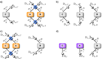
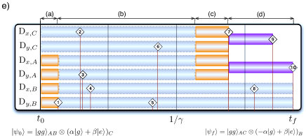
Figure 3: Steps for the teleportation protocol. A combined detection in $AB$ prepares Alice and Bob’s Bell pair (a). In (b) the beamsplitters are removed and only local flips can occur. An entangling operation between $A$ and $C$ is performed in (c) setting Alice’s qubits up for computational basis measurements. With all the beamsplitters removed, and the “i.s.” mechanism turned off, qubits $A$ and $C$ are measured in (d). A simulation of these steps is shown in (e) with diamonds indicating the occurrence of a detection event.

A major advantage of this gate over other ways to entangle qubits by monitoring spontaneously emitted photons Jakóbczyk (2002) is its scalability. In fact, despite being based on detections, our gates are unitary, allowing the creation of arrays and networks of entangled qubits. This property is essential, for example, in the implementation of a teleportation protocol or the creation of multiqubit graph states.

The teleportation steps are described in Fig. 3. In (a) Alice and Bob entangle their qubits using the scheme shown in Fig. 1.3. After a click in one of the detectors $D_{x(y),A(B)}$ the beam splitters must be removed, passing to configuration (b), where only entanglement-preserving clicks (as in Fig. 1.2-a) can be detected. The Bell measurement step starts in (c), where Alice repeats the step in (a) but now entangling her qubit with Charlie’s (the qubit in the state to be teleported). After a click in one of the combined detectors, the beam splitters are removed and the driving fields in Alice and Charlie’s qubits turned off. In this situation, shown in (d), detection in $A$ and $C$ corresponds to the scheme in Fig. 1.1 and a measurement in the computational basis is performed. The diagram in (e) represents the results of a simulation of the counts (shown by diamonds) in each detector for all the stages of the teleportation protocol. The interval between steps (a) and (c) (the duration of step (b)) was arbitrarily set to $1/\gamma$. At the end of protocol, Alice and Charlie must communicate the results of their detections to Bob, which now, in possession of the information about the measurements (in this case the 10 clicks detected), knows that the final state is $|\psi_{f}\rangle$ and he has to apply a simple Pauli operation (in this case $-\sigma_{z}$) to obtain Charlie’s original state.

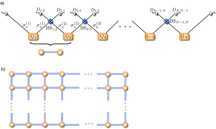
Figure 4: Generation of graph states. a) The generation of a multiqubit state equivalent to a linear cluster state can be obtained by concatenating a variant of the entangling gate shown in Fig. 1.3. In the case shown in the figure, only the $\sigma_{x}$ channels are combined at the BS while the $\sigma_{y}$ channels (not shown) should be detected independently (corresponding to the absence of ${\rm BS}_{y}$ in Fig. 1.3). (b) With extra beam-splitters, one can connect a sequence of linear graphs to build a 2D cluster state, an universal resource for quantum computations.

The generation of a multiqubit graph state, as shown in Fig. 4, follows from the parallel application of the entangling operation for every edge in the graph. All the neighbour channels (in the graph topology) are initially combined. However, since non-commuting operations are not desirable, only one of the channels, for example $\sigma_{x}$, of each qubit should be combined. The other channel is still monitored (corresponding to Fig. 1.3 without $BS_{y}$) and its clicks do not affect the overall result (they just correspond to locally redefining the logical “$0$” and “$1$”). Each time an entangling photon is detected, the corresponding standard BS is removed and subsequent photons in the same detectors locally flip the respective qubits.

For example, starting out with all $N$ qubits in the eigenstate $|0\rangle$ of $\sigma_{z}$, the generate state is

$$|\tilde{G}_{N}\rangle=\prod_{(j,k)\in G}X_{jk}^{s_{j,k}}\ |0\rangle^{\otimes N}$$ (1)

where $s_{j,k}=\pm$ depends on which detector clicks in the combined $BS_{j,k}$ channels and the $j$’s and $k$’s are chosen accordingly to the connections present in the graph. Note that the $X_{jk}^{\pm}$ gates are formally equivalent (up to local unitaries) to Controlled-Z gates used to produce usual graph states as $|G_{N}\rangle=\prod_{(j,k)\in G}cZ_{j,k}|+\rangle^{\otimes N}$. Indeed they can be rewriten as $X_{jk}^{\pm}=e^{\pm i\pi/4}X^{\mp}_{j}X^{\pm}_{k}cX_{j,k}$, where $X^{\pm}_{j}=(\mathcal{I}\pm i\sigma_{x_{j}})$ is a local unitary and $cX_{j,k}$ is the $X$ basis version of the $cZ_{j,k}$ gate. Using that $H\sigma_{x_{j}}H=\sigma_{z_{j}}$ and the fact that all gates involving $\sigma_{z}$ commute, the state in Eq. (1) can then be rewritten as:

$$|\tilde{G}_{N}\rangle=\prod_{j}U_{j}|G_{N}\rangle,$$ (2)

with $\prod_{j}U_{j}=H^{\otimes N}\prod_{(j,k)\in G}e^{s_{j,k}i\pi/4}Z^{-s_{j,k}}_{j}Z^{+s_{j,k}}_{j}$, $Z^{\pm s_{j,k}}_{j}=(\mathcal{I}\pm s_{j,k}i\sigma_{z_{j}})$ and $H$ being the usual Hadamard transformation. The state generated by our method is the usual graph-state, up to local unitaries conditioned on the clicks. It is worthy mentioning that all the measurements necessary to perform a universal one-way quantum computation are in the computational basis or comprised in the x-y plane of the Bloch sphere and can indeed be performed with the schemes presented in Fig. 1.1 and Fig. 1.2-a respectively. Given that, it can be formally shown that all the different clicks in the detectors (corresponding to different local unitaries) can be treated as the usual adaptations in the measurement basis of a given one-way algorithm. However, due to the products of Hadamards appearing in $U_{j}$ it is also necessary to introduce such transformations in our framework. This is easily achieved by the same quantum erasing principle that allows for the implementation of single qubit rotations in the x-y plane. However, in this case, an extra classical photon source is required. For example, if the propagation channel of an attenuated laser is combined in a standard beam splitter ($BS$) with the $\sigma_{y}$ output channel of a given emitting qubit $k$, then the detection of a photon after the $BS$ corresponds to applying the jump operator $(\mathcal{I}\pm i\sigma_{y_{k}})/\sqrt{2}=\exp\left(\pm i\frac{\pi}{4}\sigma_{y_{k}}\right)$ to qubit $k$, which also changes qubit $k$ from $Z$ basis to $X$ basis, and vice-versa.

The procedure to prepare graph states described above is efficient: If $\tau$ is the average time to entangle one pair (average time for one of two qubits to emit or scatter one photon), then the parallel character of our proposal implies an overhead time of the order of $\tau\log N$ for the creation of an entire graph state comprised of $N$ edges. In order to prove this, note that the generation process is completed after the last combined detector has clicked, in an instance of the famous coupon collector problem Durret:2010 . The mean value for the time of occurrence of this last edge is of the order of $\tau\log N$, where $\tau$ is the typical time for one independent detection and $N$ is the number of edges on the graph. As an example, for preparing a $2D$–cluster state of $100\times 100$ qubits it will take about $12$ times the decay time of one isolated qubit.

The results here presented are fundamentally different from other proposals that use dissipation as resources for quantum computation. There, either the interactions between qubits and reservoirs have to be carefully and dynamically engineered throughout the computation Verstraete et al. (2009); Barreiro et al. (2011), or the protocol is probabilistic Duan et al. (2001); Olmschenk et al. (2009). Furthermore the deleterious effects of natural spontaneous emission are always present. In contrast, here we consider local reservoirs and incoherent pumping that always couple to each qubit in the same way and the computation is obtained by suitably observing the out-coming photons. Therefore, there is no need for direct action neither on the qubits nor on the couplings and the computation is naturally protected from spontaneous emission. Note also that in our case the process as a whole is stochastic but the computation is not probabilistic: each realization produces one of many possible versions of the desired graph state, each version differing from the others by local Pauli operations that can be absorbed in the adaptation of measurement basis required by a given computational algorithm.

We have investigated the computational power of quantum trajectories and proved that one can implement any algorithm by suitably observing the photons that are spontaneously emitted and inelastically scattered by a multiqubit system. The results show that a natural reservoir that destroys quantum coherence when unobserved can be unravelled into quantum trajectories with full quantum computational power. From a fundamental point of view, one can interpret this scheme as a careful and efficient selection of the set of quantum trajectories that performs a desired computation out of the infinitude of possible unravellings allowed for that given environment interaction. Our scheme suits both circuit and measurement based quantum computation and we believe that recent technological developments in $1$-D systems Claudon et al. (2010); Schoelkopf and Girvin (2008); Hwang et al. (2009) will allow it to be tested in the near future.

The concepts here presented may also significantly contribute to hybrid strategies to produce a quantum computer, for example, by combining the here introduced entangling gates with more traditional techniques to perform local operations. In that respect, it is particularly encouraging the rather efficient way to produce graph states by detecting the emitted and scattered photons.

Other interesting directions of investigation are the integration of the usual quantum error correcting codes in this computational approach, the development of new strategies to protect quantum information in reservoir monitoring schemes, and the connection with problems of percolation. Finally, the intrinsic random nature of the clicks also indicates that the same scheme could be used to generate random quantum circuits, $t$-designs and quantum walks, all useful methods to study many-body quantum systems.

This work was conceived and majorly developed during the “Quantum Information” session of the “Centro de Ciencias de Benasque Pedro Pascual” in Benasque, Spain. MFS and MTC thank CNPq and Fapemig for financial support. R. C. was funded by the Q-Essence project. This work is part of the INCT-IQ from CNPq, Brazil. It was also supported by the Australian Research Council Centre of Excellence for Quantum Computation and Communication Technology (project number CE110001027).

References

- Nielsen and Chuang (2000) M. A. Nielsen and I. L. Chuang, Quantum computation and quantum information (Cambridge University Press, 2000).
- Raussendorf and Briegel (2001) R. Raussendorf and H. J. Briegel, Phys. Rev. Lett. 86, 5188 (2001).
- Raussendorf et al. (2003) R. Raussendorf, D. E. Browne, and H. J. Briegel, Phys. Rev. A 68, 022312 (2003).
- Giulini and et al. (1996) D. Giulini and et al., Decoherence and the appearance of a classical world in quantum theory (Springer Press, Berlin, 1996).
- Carmichael (1993) H. Carmichael, An open systems approach to quantum optics, Lecture Notes in Physics m 18 (Springer-Verlag, Berlin, 1993).
- Sauter et al. (1986) T. Sauter, W. Neuhauser, R. Blatt, and P. E. Toschek, Phys. Rev. Lett. 57, 1696 (1986).
- Nagourney et al. (1986) W. Nagourney, J. Sandberg, and H. Dehmelt, Phys. Rev. Lett. 56, 2797 (1986).
- Gleyzes et al. (2007) S. Gleyzes, S. Kuhr, C. Guerlin, J. Bernu, S. Deleglise, U. Busk Hoff, M. Brune, J.-M. Raimond, and S. Haroche, Nature 446, 297 (2007).
- Carvalho and Santos (2011) A. R. R. Carvalho and M. F. Santos, New Journal of Physics 13, 013010 (2011).
- Scully and Drühl (1982) M. O. Scully and K. Drühl, Phys. Rev. A 25, 2208 (1982).
- M. O. Scully (1991) H. W. M. O. Scully, Berthold-Georg Englert, Nature 351, 111 (1991).
- Loss and DiVincenzo (1998) D. Loss and D. P. DiVincenzo, Phys. Rev. A 57, 120 (1998).
- Neumann et al. (2008) P. Neumann, N. Mizuochi, F. Rempp, P. Hemmer, H. Watanabe, S. Yamasaki, V. Jacques, T. Gaebel, F. Jelezko, and J. Wrachtrup, Science 320, 1326 (2008).
- DiVincenzo (2010) D. DiVincenzo, Nat Mater 9, 468 (2010).
- Brouri et al. (2000) R. Brouri, A. Beveratos, J.-P. Poizat, and P. Grangier, Opt. Lett. 25, 1294 (2000).
- Makhlin et al. (2001) Y. Makhlin, G. Schön, and A. Shnirman, Rev. Mod. Phys. 73, 357 (2001).
- Vion et al. (2002) D. Vion, A. Aassime, A. Cottet, P. Joyez, H. Pothier, C. Urbina, D. Esteve, and M. H. Devoret, Science 296, 886 (2002).
- Chiorescu et al. (2003) I. Chiorescu, Y. Nakamura, C. J. P. M. Harmans, and J. E. Mooij, Science 299, 1869 (2003).
- Barth et al. (2009) M. Barth, N. Nüsse, B. Löchel, and O. Benson, Opt. Lett. 34, 1108 (2009).
- Wolters et al. (2010) J. Wolters, A. W. Schell, G. Kewes, N. Nusse, M. Schoengen, H. Doscher, T. Hannappel, B. Lochel, M. Barth, and O. Benson, Applied Physics Letters 97, 141108 (2010), ISSN 00036951.
- Nadj-Perge et al. (2010) S. Nadj-Perge, S. M. Frolov, E. P. A. M. Bakkers, and L. P. Kouwenhoven, Nature 468, 1084 (2010).
- Jacques et al. (2007) V. Jacques, E. Wu, F. Grosshans, F. Treussart, P. Grangier, A. Aspect, and J.-F. Roch, Science 315, 966 (2007).
- Jakóbczyk (2002) L. Jakóbczyk, Journal of Physics A: Mathematical and General 35, 6383 (2002).
- (24) R. Durret, Probability: Theory and Examples (Cambridge, 2010).
- Verstraete et al. (2009) F. Verstraete, M. M. Wolf, and J. Ignacio Cirac, Nat Phys 5, 633 (2009).
- Barreiro et al. (2011) J. T. Barreiro, M. Muller, P. Schindler, D. Nigg, T. Monz, M. Chwalla, M. Hennrich, C. F. Roos, P. Zoller, and R. Blatt, Nature 470, 486 (2011).
- Duan et al. (2001) L. M. Duan, M. D. Lukin, J. I. Cirac, and P. Zoller, Nature 414, 413 (2001).
- Olmschenk et al. (2009) S. Olmschenk, D. N. Matsukevich, P. Maunz, D. Hayes, L.-M. Duan, and C. Monroe, Science 323, 486 (2009).
- Claudon et al. (2010) J. Claudon, J. Bleuse, N. S. Malik, M. Bazin, P. Jaffrennou, N. Gregersen, C. Sauvan, P. Lalanne, and J.-M. Gerard, Nat Photon 4, 174 (2010).
- Schoelkopf and Girvin (2008) R. J. Schoelkopf and S. M. Girvin, Nature 451, 664 (2008).
- Hwang et al. (2009) J. Hwang, M. Pototschnig, R. Lettow, G. Zumofen, A. Renn, S. Gotzinger, and V. Sandoghdar, Nature 460, 76 (2009).