Nonparametric Bayesian Estimation of Periodic Lightcurves

Abstract

Many astronomical phenomena exhibit patterns that have periodic behavior. An important step when analyzing data from such processes is the problem of identifying the period: estimating the period of a periodic function based on noisy observations made at irregularly spaced time points. This problem is still a difficult challenge despite extensive study in different disciplines. This paper makes several contributions toward solving this problem. First, we present a nonparametric Bayesian model for period finding, based on Gaussian Processes (GP), that does not make assumptions on the shape of the periodic function. As our experiments demonstrate, the new model leads to significantly better results in period estimation especially when the lightcurve does not exhibit sinusoidal shape. Second, we develop a new algorithm for parameter optimization for GP which is useful when the likelihood function is very sensitive to the parameters with numerous local minima, as in the case of period estimation. The algorithm combines gradient optimization with grid search and incorporates several mechanisms to overcome the high computational complexity of GP. Third, we develop a novel approach for using domain knowledge, in the form of a probabilistic generative model, and incorporate it into the period estimation algorithm. Experimental results validate our approach showing significant improvement over existing methods.

1. Introduction

Many astronomical phenomena exhibit periodic behavior. Discovering their period and the periodic pattern they exhibit is an important task toward understanding their behavior. A significant effort has been devoted to the analysis of lightcurves from periodic variable stars. For example, the top part of Figure (1) shows the magnitude of a light source over time. The periodicity of the light source is not obvious before we fold it. However, as the bottom part illustrates, once folded with the right period we get convincing evidence of periodicity. The object in this figure is classified as an eclipsing binary (EB). Other sources show periodic variability due to processes internal to the star (Petit, 1987).

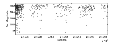
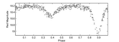
Figure 1.— Top: brightness of an eclipsing binary star over time; Bottom: brightness versus phase.

The problem of period estimation from noisy and irregularly sampled observations has been studied before in several disciplines. Most approaches identify the period by some form of grid search. That is, the problem is solved by evaluating a criterion $\Phi$ at a set of trial periods $\{p\}$ and selecting the period $p$ that yields the best value for $\Phi(p)$. The commonly-used techniques vary in the form and parametrization of $\Phi$, the evaluation of the fit quality between model and data, the set of trial periods searched, and the complexity of the resulting procedures. Two methods we use as baselines in our study are the LS periodogram (Scargle, 1982; Reimann, 1994) and the phase dispersion minimization (PDM) (Stellingwerf, 1978), both known for their success in empirical studies. The LS method is relatively fast and is equivalent to maximum likelihood estimation under the assumption that the function has a sinusoidal shape. It therefore makes a strong assumption on the shape of the underlying function. On the other hand, PDM makes no such assumptions and is more generally applicable, but it is slower and is less often used in practice. A more extensive discussion of related work is given in Section 5.

The paper makes several contributions toward solving the period estimation problem. First, we present a new model for period finding, based on Gaussian Processes (GP), that does not make strong assumptions on the shape of the periodic function. In this context, the period is a hyperparameter of the covariance function of the GP and accordingly the period estimation is cast as a model selection problem for the GP. As our experiments demonstrate, the new model leads to significantly better results compared to LS when the target function is non-sinusoidal. The model also significantly outperforms PDM when the sample size is small.

Second, we develop a new algorithm for period estimation within the GP model. In the case of period estimation the likelihood function is not a smooth function of the period parameter. This results in a difficult estimation problem which is not well explored in the GP literature (Rasmussen & Williams, 2005). Our algorithm combines gradient optimization with grid search and incorporates several mechanisms to improve the complexity over the naive approach.

In particular we propose and evaluate: an approximation using a two level grid search, approximation using limited cyclic optimization, a method using sub-sampling and averaging, and a method using low-rank Cholesky approximations. An extensive experimental evaluation using artificial data identifies the most useful approximations and yields a robust algorithm for period finding.

Third, we develop a novel approach for using astrophysics knowledge, in the form of a probabilistic generative model, and incorporate it into the period estimation algorithm. In particular, we propose to employ the generative model to bias the selection of periods by using it as a prior over periods or as a post-processing selection criterion choosing among periods ranked highly by the GP. The resulting algorithm is applied and evaluated on astrophysics data showing significantly improved performance over previous work.

The next section provides some technical background and defines the period estimation problem as GP inference. The following three sections present our algorithm, report on experiments evaluating it and applying it to astrophysics data, and discuss related work. The final section concludes with a summary and directions for future work.

2. Preliminaries: GP for Period Finding

This section provides technical background on GPs and their optimization procedures and defines the period finding problem in this context.

Throughout the paper, scalars are denoted using italics, as in $x,y\in{\rm I\!R}$; vectors and matrices use lowercase and capital bold typeface, as in $\bm{x},\bm{y},\mathbf{K},\mathbf{A}$, and $x_{i}$ denotes the $i$th entry of $\bm{x}$. For a vector $\bm{x}$ and real valued function $f:{\rm I\!R}\rightarrow{\rm I\!R}$, we extend the notation for $f$ to vectors so that $f(\bm{x})=[f(x_{1}),\cdots,f(x_{n})]^{\mathrm{T}}$ where the superscript $\mathrm{T}$ stands for transposition. $\mathbb{I}$ is the identity matrix.

2.1. Gaussian Processes

This section gives a brief review of Gaussian processes regression. A more extensive introduction can be found in (Rasmussen & Williams, 2005; Bishop, 2006).

We start with the following regression model,

$$y=f_{\bm{w}}(\bm{x})+\epsilon$$ (1)

where $f_{\bm{w}}(x)$ is the regression function with parameter $\bm{w}$ and $\epsilon$ is iid Gaussian noise. For example, in linear regression $f_{\bm{w}}(\bm{x})=\bm{w}^{T}\bm{x}$ and therefore $y\sim N(\bm{w}^{T}\bm{x}^{*},1/\sigma^{2})$. Given the data $\mathcal{D}=\{\bm{x}_{i},y_{i}\},i=1,\cdots,N$, one wishes to infer $\bm{w}$ and the basic approach is to maximize the likelihood $\mathcal{L}(\bm{w},\mathcal{D})=\Pr(\mathcal{D}|\bm{w})$.

In Bayesian statistics, the parameter $\bm{w}$ is assumed to have a prior probability $\Pr(\bm{w})$ which encodes the prior belief on the parameter. The inference task becomes calculating the posterior distribution over $\bm{w}$, which, using the Bayesian formula, is given as

$$\Pr(\bm{w}|\mathcal{D})\propto\Pr(\mathcal{D}|\bm{w})\Pr(\bm{w}).$$ (2)

The predictive distribution for a new observation $\bm{x}^{*}$ is given by

$$\Pr(f(\bm{x}^{*})|\mathcal{D})=\int\Pr(f(\bm{x}^{*})|\bm{w})\Pr(\bm{w}|\mathcal{D})d\bm{w}.$$ (3)

Returning to linear regression, the common model assumes that the prior for $\bm{w}$ is a zero-mean multivariate Gaussian distribution, and the posterior turns out to be multivariate Gaussian as well. In contrast with many Bayesian formulations, the use of GP often allows for simple inference or calculation of desired quantities because of properties of multivariate Gaussian distributions and corresponding facts from linear algebra.

This approach can be made more general using a nonparametric Bayesian model. In this case we replace the parametric latent function $f_{\bm{w}}$ by a stochastic process $f$ where $f$’s prior is given by a Gaussian process. A GP is specified by a mean function (assumed to be zero in this paper) and covariance function $\mathcal{K}(\cdot,\cdot)$. This allows us to specify a prior over functions $f$ such that the distribution induced by $f$ over any finite sample is normally distributed. More precisely, the GP regression model with zero mean and covariance function $\mathcal{K}(\cdot,\cdot)$ is as follows. Given sample points $[\bm{x}_{1},\ldots,\bm{x}_{n}]^{T}$ let $\mathbf{K}=(\mathcal{K}(\bm{x}_{i},\bm{x}_{j}))_{i,j}$. The induced distribution on the values of the function at the sampling points is

$$\mathbf{f}\triangleq[f(\bm{x}_{{}_{1}}),\cdots,f(\bm{x}_{{}_{N}})]^{\mathrm{T}}\sim\mathcal{N}(\mathbf{0},\mathbf{K}),$$ (4)

where $\mathcal{N}$ denotes the multivariate normal distribution. Now assuming that $y_{i}$ is generated from $f(\bm{x}_{{}_{i}})$ using iid noise as in Equation (1) and denoting $\bm{y}=[y_{1},\ldots,y_{n}]^{T}$ we get that $\bm{y}\sim\mathcal{N}(\mathbf{0},\mathbf{K}+\sigma^{2}\mathbb{I})$ and the joint distribution is given by

$$\begin{bmatrix}\mathbf{f}\\ \bm{y}\end{bmatrix}\sim\cal{N}\left(\begin{bmatrix}\mathbf{0}\\ \mathbf{0}\\ \end{bmatrix},\begin{bmatrix}\mathbf{K}&\mathbf{K}\\ \mathbf{K}&\mathbf{K}+\sigma^{2}\mathbb{I}\end{bmatrix}\right).$$ (5)

Using properties of multivariate Gaussians we can see that the posterior distribution $\mathbf{f}|\bm{y}$ is given by

$$\Pr(\mathbf{f}|\mathcal{D})=\mathcal{N}(\mathbf{K}\,(\sigma^{2}\mathbb{I}+\mathbf{K})^{-1}\,\bm{y}\,,\,\sigma^{2}\,\,(\sigma^{2}\mathbb{I}+\mathbf{K})^{-1}\mathbf{K}).$$ (6)

Similarly, the predictive distribution for some test point $\bm{x}_{*}$ distinct from the training examples is given by

$$\begin{split}&\Pr(f(\bm{x}_{*})|\bm{x}_{*},\mathcal{D})=\int\Pr(f(\bm{x}_{*})|\bm{x}_{*},f)\Pr(f|\mathcal{D})df\\ &=\mathcal{N}\bigg{(}\mathbf{k}(\bm{x}_{*})^{\mathrm{T}}(\sigma^{2}\mathbb{I}+\mathbf{K})^{-1}\bm{y},\\ &\qquad\qquad\mathcal{K}(\bm{x}_{*},\bm{x}_{*})-\mathbf{k}(\bm{x}_{*})^{\mathrm{T}}(\sigma^{2}\mathbb{I}+\mathbf{K})^{-1}\mathbf{k}(\bm{x}_{*})\bigg{)}\end{split}$$ (7)

where $\mathbf{k}(\bm{x}_{*})=[\mathcal{K}(\bm{x}_{1},\bm{x}_{*}),\cdots,\mathcal{K}(\bm{x}_{N},\bm{x}_{*})]^{\mathrm{T}}$.

Figure 2 illustrates GP regression, by showing how a finite sample induces a posterior over functions and their values for new sample points.

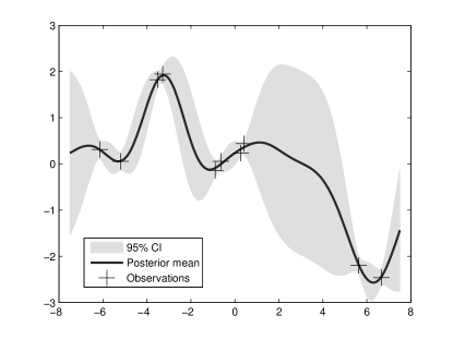
Figure 2.— Illustration of prediction with GP regression. The data points $\mathcal{D}=\{\bm{x}_{i},y_{i}\}$ are given by the crosses. The shaded area represents the pointwise 95% confidence region of the predictive distribution. As can be seen from Equation 7, GP regression can be seen to perform a variant of kernel regression where $f(\bm{x}_{*})$ is a weighted average of all the measurements $\bm{y}$. While the values of the weights are obscured because of the inverse of the covariance matrix in that expression, one can view this roughly by an analogy to nearest neighbor regression where the mean of $f(\bm{x}*)$ is affected more by the measurements whose sampling points are close to $\bm{x}^{*}$ and the variance of $f(\bm{x}^{*})$ is small if $\bm{x}^{*}$ is surrounded by measurements. A deeper discussion of the equivalent kernel is given in (Rasmussen & Williams, 2005).

2.2. Problem Definition

In the case of period estimation the sample points $\bm{x}_{i}$ are scalars $x_{i}$ representing the corresponding time points, and we denote $\bm{x}=[x_{1},\ldots,x_{n}]^{T}$. The underlying function $f(\cdot)$ is periodic with unknown period $p$ and corresponding frequency $w=1/p$. To model the periodic aspect we use a GP with a periodic covariance function

$$\mathcal{K}_{\bm{\theta}}(x_{i},x_{j})=\beta\exp{\left\{-\frac{2\sin^{2}\left(w\pi(x_{i}-x_{j})\right)}{\ell^{2}}\right\}},$$ (8)

where the set of hyperparameters of the covariance function is given by $\bm{\theta}=\{\beta,w,\ell\}$. It can be easily seen that any $f$ generated by $\mathcal{K}_{\bm{\theta}}$ is periodic with period $1/w$. Figure (3) illustrates the role of the other two hyperparameters. We can see that $\beta$ controls the magnitude of the sampled functions. At the same time, $\ell$ which is called characteristic length determines how sharp the variation is between two points.

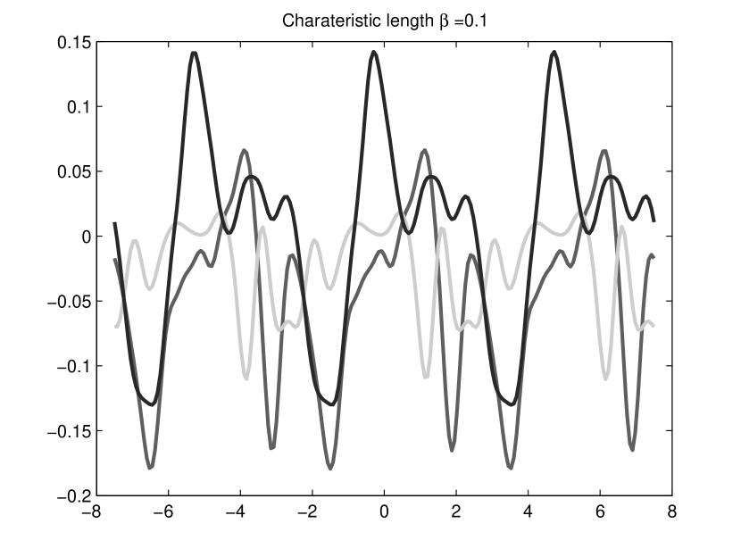
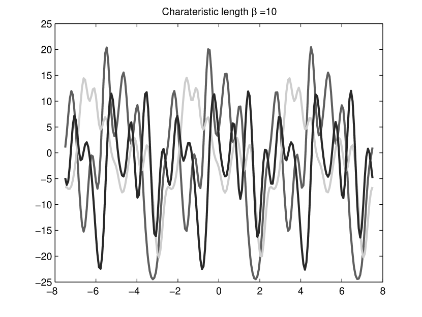
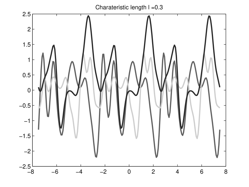
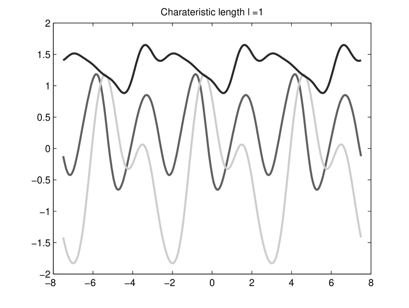
Figure 3.— Sample functions from a GP with covariance function in Equation (8) where the period is fixed to be 5, i.e. $w=0.2$. Top row: $\beta=0.1$ vs $\beta=10$ while $\ell$ is fixed to be 1. Bottom row: $\ell=0.3$ vs $\ell=1$ with $\beta=0.3$.

In our problem each star has its own period and shape and therefore each has its own set of hyperparameters. Our model, thus, assumes that the following generative process is the one producing the data. For each time series $j$ with arbitrary sample points $\bm{x}^{j}=[x_{1}^{j},\cdots,x_{N_{j}}^{j}]^{T}$, we first draw

$$f_{j}|\theta_{j}\sim\mathcal{GP}(0,\mathcal{K}_{\bm{\theta}_{j}}).$$ (9)

Then, given $\bm{x}^{j}$ and $f_{j}$ we sample the observations

$$\bm{y}^{j}\sim\mathcal{N}(f_{j}(\bm{x}^{j}),\sigma^{2}\mathbb{I}).$$ (10)

Denote the complete set of parameters by $\mathcal{M}=\{\bm{\theta},\sigma^{2}\}$. For each time series $j$, the inference task is to select the correct model for the data $\{\bm{x}^{j},\bm{y}^{j}\}$, that is, to find $\mathcal{M}$ that best describes the data. This is the main computational problem studied in this paper. The next subsection reviews two standard approaches for this problem.

Before presenting these we clarify two methodological issues. First, notice that our model assumes homogeneous noise $\mathcal{N}(0,\sigma^{2})$, i.e. the observation error for each $x_{i}$ is the same. Experimental results on the astronomy data (not shown here) show that $\sigma^{2}$ estimated from the data is very close to the mean of the recorded observation errors, and therefore there is no advantage in explicitly modeling the recorded observation errors.

Second, as defined above our task is to find the full set of parameters $\mathcal{M}$. Therefore, our framework and induced algorithms can estimate the underlying function, $f$, through the posterior mean $\hat{f}$, and thus yield a solution for the regression problem – predicting the value of the function at unseen sample points. However, our main goal and interest in solving the problem is to infer the frequency $w$ where the other parameters are less important. Therefore, a large part of the evaluation in the paper focuses on accuracy in identifying the frequency, although we also report results on prediction accuracy for the regression problem.

2.3. Model selection

2.3.1 Marginal Likelihood

The standard Bayesian approach is to identify the hyper-parameters that maximize the marginal likelihood. More precisely, we try to find $\mathcal{M}^{*}$ such that

$$\mathcal{M}^{*}=\underset{\mathcal{M}}{\text{argmax}}\left[\log\left[\Pr(\bm{y}|\bm{x};\mathcal{M})\right]\right]$$ (11)

where the marginal likelihood is given by

$$\begin{split}\log\Pr(\bm{y}|\bm{x};\mathcal{M})&=\log\left(\int\Pr(\bm{y}|f,\bm{x};\mathcal{M})\Pr(f|\bm{x};\mathcal{M})\,df\right)\\ &=-\frac{1}{2}\bm{y}^{T}(\bm{K}+\sigma^{2}\mathbb{I})^{-1}\bm{y}\\ &\quad-\frac{1}{2}\log|\bm{K}+\sigma^{2}\mathbb{I}|^{-1}-\frac{n}{2}\log 2\pi\end{split}$$ (12)

and Equation (12) holds because $\bm{y}\sim\mathcal{N}(\mathbf{0},\bm{K}+\sigma^{2}\mathbb{I})$ (Rasmussen & Williams, 2005). Typically, one can optimize the marginal likelihood by calculating the partial derivative of the marginal likelihood w.r.t. the hyper-parameters and optimizing the hyper-parameters using gradient based search (Rasmussen & Williams, 2005). As we show below, gradients alone cannot be used to solve our problem completely and therefore our algorithm elaborates and improves over this approach. We do, however, use the conjugate gradients optimization as a basic step in our algorithm. The partial derivative of Equation (12) w.r.t. the parameter $\theta_{j}$ is  (Rasmussen & Williams, 2005)

$$\begin{split}\frac{\partial}{\partial\theta_{j}}\log\Pr(\bm{y}|\bm{x};\mathcal{M})&=\text{Tr}\left(\left(\alpha\alpha^{T}-\bm{K}_{\sigma}^{-1}\right)\frac{\partial{\bm{K}_{\sigma}}}{\partial\theta_{j}}\right)\end{split}$$ (13)

where $\bm{K}_{\sigma}=\bm{K}+\sigma^{2}\mathbb{I}$ and $\alpha=\bm{K}_{\sigma}^{-1}\bm{y}$.

2.3.2 Cross-Validation

An alternative approach (Rasmussen & Williams, 2005) picks hyperparameter $\mathcal{M}$ by minimizing the empirical loss on a hold out set. This is typically done with a leave-one-out (LOO) formulation, which uses a single observation from the original sample as the validation data, and the remaining observations as the training data. The process is repeated such that each observation in the sample is used once as the validation data. To be precise, we choose the hyperparameter $\cal{M}^{*}$ such that

$$\mathcal{M}^{*}=\underset{\mathcal{M}}{\text{argmin}}\sum_{i=1}^{n}(y_{i}-\hat{f}_{-i}(x_{i}))^{2}$$ (14)

where $\hat{f}_{-i}$ is defined as the posterior mean given the data $\{\bm{x}_{-i},\bm{y}_{-i}\}$ in which the subscript $-i$ means all but the $i$th sample, that is,

$$\hat{f}_{-i}(x)=\mathcal{K}(\bm{x}_{-i},x)^{T}\left(\bm{K}_{-i}+\sigma^{2}\mathbb{I}\right)^{-1}\bm{y}_{-i}.$$ (15)

It can be shown that this computation can be simplified (Rasmussen & Williams, 2005) using the fact that

$$y_{i}-\hat{f}_{-i}(x_{i})=\frac{\left[(\bm{K}+\sigma^{2}\mathbb{I})^{-1}\bm{y}\right]_{i}}{\left[(\bm{K}+\sigma^{2}\mathbb{I})^{-1}\right]_{ii}}$$ (16)

where $[\cdot]_{i}$ is the $i$th entry of the vector and $[\cdot]_{ii}$ denotes the $(i,i)$th entry of the matrix.

3. Algorithm

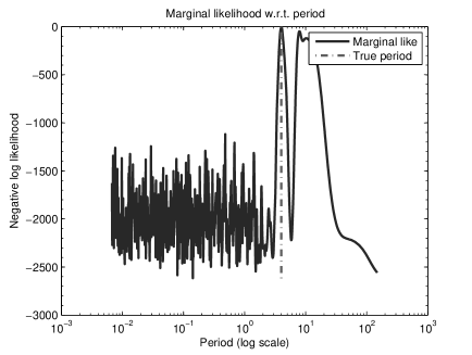
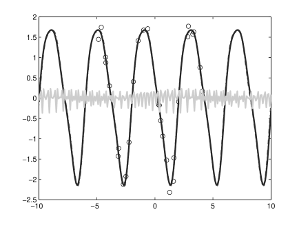
Figure 4.— Illustration of sensitivity of the marginal likelihood. A light curve is generated using the GP model with parameters $\beta=1$, $w=0.25$, and $\ell=1$. Left: The marginal likelihood function versus the period, where the dotted line indicates the true period. Right: The black circles are the observations and the dotted line (covered by the dark estimated curve) is the true function. The dark line which covers the true curve and the light line are the learned regression functions given two different starting points of $w$.

1:  Initialize the parameters randomly. 2:  repeat 3:        Jointly find $\tilde{w},\beta^{*},\ell^{*},\sigma^{*}$ that maximize Equation (12) using conjugate gradients. 4:        for all $w$ in a coarse grid set $\mathcal{C}$ do 5:              Calculate the marginal likelihood Equation (12) or the LOO Error Equation (14) using $\beta^{*},\ell^{*},\sigma^{*}$. 6:        end for 7:        Set $w$ to the best value found in the for loop. 8:  until Number of iterations reaches $L_{1}$ ($L_{1}=2$ by default) 9:  Record the Top $K$ ($K=10$ by default) frequencies $\mathcal{W}^{*}$ found in the last run of for loop (lines 4-6). 10:  repeat 11:        Jointly find $\tilde{w},\beta^{*},\ell^{*},\sigma^{*}$ that maximize Equation (12) using conjugate gradients. 12:        for all $w$ in a fine grid set $\mathcal{F}$ that covers $\mathcal{W}^{*}$ do 13:              Calculate the marginal likelihood Equation (12) or the LOO Error Equation (14) using $\beta^{*},\ell^{*},\sigma^{*}$. 14:        end for 15:        Set $w$ to the best value found in the for loop. 16:  until Number of iterations reaches $L_{2}$ ($L_{2}=2$ by default) 17:  Output the frequency $w^{*}$ that maximizes the marginal likelihood or minimizes the LOO Error in the last run of for loop (lines 11-13).

Figure 5.— Hyperparameter Optimization Algorithm

We start by demonstrating experimentally that gradient based methods are not sufficient for period estimation. We generate synthetic data and maximize the marginal likelihood w.r.t. $\bm{\theta}=\{\beta,w,\ell\}$ using conjugate gradients. For this experiment, 30 samples in the interval $[-10,10]$ are generated according to the periodic covariance function in Equation (8) with $\bm{\theta}=[1,0.25,1]$. Fixing $\beta,\ell$ to their correct values, the marginal likelihood w.r.t. the period $1/w$ is shown in Figure 4 left. The figure shows that the marginal likelihood has numerous local minima in the high frequency (small period) region that have no relation to the true period. Figure 4 right shows two functions with the learned parameters based on different starting points (initial values).

The function plotted in dark color estimates the true function correctly while the one in light color does not. This is not surprising because from Figure 4 left, we can see that there is only a small region of initial points from which the algorithm can find the correct period. We repeated this experiment using several other periodic functions with similar results. These preliminary experiments illustrate two points:

• When other parameters are known, the marginal likelihood function is maximized at the correct period, showing that in principle we can find the correct period by optimizing the marginal likelihood.

• On the other hand, it is not possible to identify the period using only gradient based search.

Therefore, as in previous work (Reimann, 1994; Hall et al., 2000), our algorithm uses grid search for the frequency. The grid used for the search must be sufficiently fine to detect the correct frequency and this implies high computational complexity. We therefore follow a two level grid search for frequency where the coarse grid must intersect the smooth region of the true maximum and the fine grid can search for the maximum itself. The two-level search significantly reduces the computational cost. Our algorithm, presented in Figure 5 combines this with gradient based optimization of the other parameters. There are several points that deserve further discussion, as follows:

1. In step 3, we can successfully maximize the marginal likelihood w.r.t. $\beta,\ell$ and $\sigma^{2}$ using the conjugate gradients method, but this approach does not work for the frequency $w$. The reason is that the objective function is highly sensitive w.r.t. $w$ and the gradient is not useful for finding the global maximum. This property justifies the structure of our algorithm. This issues has been observed before and grid search (in particular using two stages) is known to be the most effective solution (Reimann, 1994; Hall et al., 2000).

2. Our algorithm uses cyclic optimization estimating $w$, $\sigma$, $\beta$, $\ell$. That is to say, we fix other parameters $\sigma$, $\beta$, $\ell$ and optimize $w$ and then optimize $\sigma$, $\beta$, $\ell$ when $w$ is fixed. We keep doing this iteratively but use a small number of iterations (in our experiments, the default number of iterations is 2). A more complete algorithm would iterate until convergence but this incurs a large computational cost. Our experiments demonstrate that a small number of iterations is sufficient.

3. In steps 3 and 11 we incorporate $w$ into the joint optimization of the marginal likelihood. This yields better results than optimizing w.r.t. the other parameters with fixed $w$. This shows that the gradient of $w$ sometimes still provides useful information locally, although the obtained optimal value $\tilde{w}$ is discarded.

4. We use an adaptive search in the frequency domain, where at the first stage we use a coarse grid and later a fine grid search is performed at the neighbors of the best frequencies previously found. By doing this, the computational cost is dramatically reduced while the accuracy of the algorithm is still guaranteed.

Two additional approximations are introduced next, specifically targeting the coarse and fine grids respectively and using observations that are appropriate in each case.

3.1. Ensemble Subsampling

The coarse grid search in lines 4-6 of the algorithm needs to compute the covariance matrix w.r.t. each frequency in $\mathcal{C}$ and invert the corresponding covariance matrix, and therefore the total time complexity is $\mathcal{O}\left(|\mathcal{C}|N^{3}\right)$. In addition, different stars do not share the same sampling points. Therefore the covariance matrix and its inverse cannot be cached to be used on all stars. The computational cost is too high when the coarse grid has a large cardinality. Our observation here is that it might suffice to get an approximation of the likelihood at this stage of the algorithm, because additional fine grid search is done in the next stage.

Therefore, to reduce the time complexity, we propose an ensemble approach that combines the marginal likelihood of several subsampled times series. The idea (Protopapas et al., 2005) is that the correct period will get a high score for all sub-samples, but wrong periods that might score well on some sub-samples (and be preferred to others due to outliers) will not score well on all of them and will thus not be chosen. For the approximation, we sub-sample the original time series such that it only contains a fraction $f$ of the original time points, repeating the process $R$ times. The marginal likelihood score is the average over the $R$ repetitions. Our experiments justify default settings of $f=15\%$ (with the additional constraint that $30\leq f\leq 40$) and $R=10$. This approximation reduces the time complexity to $\mathcal{O}\left(|\mathcal{C}|\times R\times(fN)^{3}\right)$.

3.2. First Order Approximation with Low Rank Approximation

Similar to the previous case, the time complexity of fine grid search is $\mathcal{O}(|\mathcal{F}|N^{3})$. In this case we can reduce the constant factor in the $\mathcal{O}(N^{3})$ term. Notice that in step 13, other parameters are fixed and the grid is fine so that the marginal likelihood is a smooth function of $w$. Suppose we have $w_{0},w_{1}\in\mathcal{F}$ where $\cal{F}$ is the fine grid and $\Delta w=|w_{0}-w_{1}|<\epsilon$, where $\epsilon$ is a predefined threshold. Then, given $\bm{K}_{w_{0}}$, the covariance matrix w.r.t. $w_{0}$, we can get $\bm{K}_{w_{1}}$ by its Taylor expansion as

$$\bm{K}_{w_{1}}=\bm{K}_{w_{0}}+\frac{\partial\bm{K}}{\partial w}(w_{0})\Delta w+o(\epsilon^{2}).$$ (17)

Denote $\widetilde{\bm{K}}=\frac{\partial\bm{K}}{\partial w}(w_{0})$ where $\widetilde{\bm{K}}\Delta w$ can be seen as a small perturbation to $\bm{K}_{w_{0}}$. At first look, the Sherman-Morrison-Woodbury formula (Bishop, 2006) appears to be suitable for calculating the update of the inverse efficiently. Unfortunately, preliminary experiments (not shown here) indicated that this method fails due to numeric instability. Instead, we use an update for the Cholesky factors of the matrix and calculate the inverse through these. Namely, given the Cholesky decomposition of $\bm{K}_{w_{0}}=\bm{L}\bm{L}^{T}$ we calculate $\widetilde{\bm{L}}$ such that $\widetilde{\bm{L}}\widetilde{\bm{L}}^{T}=\bm{K}_{w_{0}}+\Delta w\widetilde{\bm{K}}\approx\bm{K}_{w_{1}}$. Details of this construction are given in the appendix.

3.3. Astrophysical Input Improvements

For some cases we may have further information on the type of periodic functions one might expect. We propose to use such information to bias the selection of periods, by using it to induce a prior over periods or as a post-processing selection criterion. The details of these steps are provided in the next section.

4. Experiments

This section evaluates the various algorithmic ideas using synthetic and astrophysics data and then applies the algorithm to a different set of lightcurves. Our implementation of the algorithms makes use of the gpml package (Rasmussen & Nickisch, 2010).

4.1. Synthetic data

In this section, we evaluate the performance of several variants of our algorithm, study the effects of its parameters, and compare it to the two most used methods in the literature: the LS periodogram (LS) (Lomb, 1976) and phase dispersion minimization (PDM) (Stellingwerf, 1978).

The LS method (Lomb, 1976) chooses $w$ to maximize the periodogram defined as:

$$\begin{split}P_{LS}(\omega)&=\frac{1}{2}\Bigg{\{}\frac{[\sum y_{j}\cos(\eta_{j})]^{2}}{\sum\cos^{2}(\eta_{j})}+\frac{[\sum y_{j}\sin(\eta_{j})]^{2}}{\sum\sin^{2}(\eta_{j})}\Bigg{\}},\end{split}$$ (18)

where $\eta_{j}=\omega(x_{j}-\tau)$. The phase $\tau$ (that depends on $\omega$) is defined as the value satisfying $\tan(2\omega\tau)=\frac{\sum\sin(2\omega x_{j})}{\sum\cos(2\omega x_{j})}.$ As shown by (Reimann, 1994), LS fits the data with a harmonic model using least-squares.

In the PDM method, the period producing the least possible scatter in the derived light curve is chosen. The score for a proposed period can be calculated by folding the light curve using the proposed period, dividing the resulting observation phases into bins, and calculating the local variance within each bin, $\sigma^{2}=\frac{\sum_{j}(y_{j}-\bar{y})^{2}}{N-1},$ where $\bar{y}$ is the mean value within the bin and the bin has $N$ samples. The total score is the sum of variances over all the bins. This method has no preference for a particular shape (e.g., sinusoidal) for the curve.

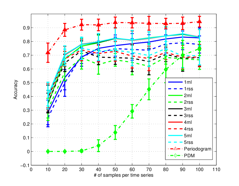
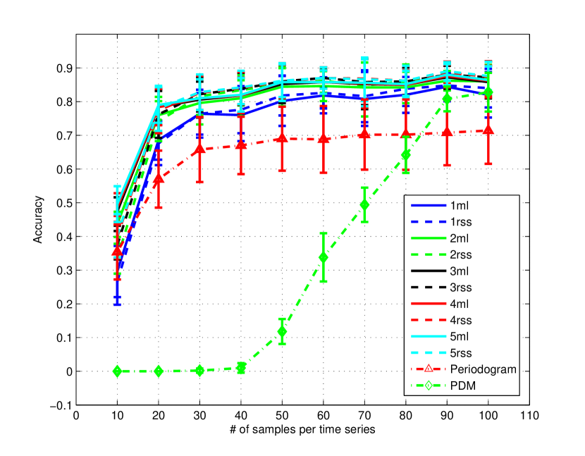
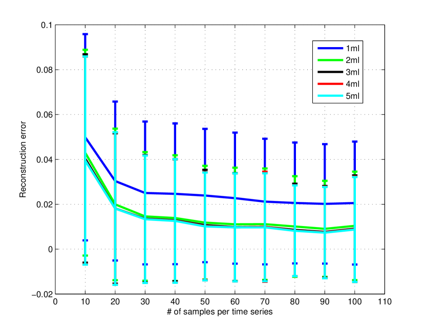
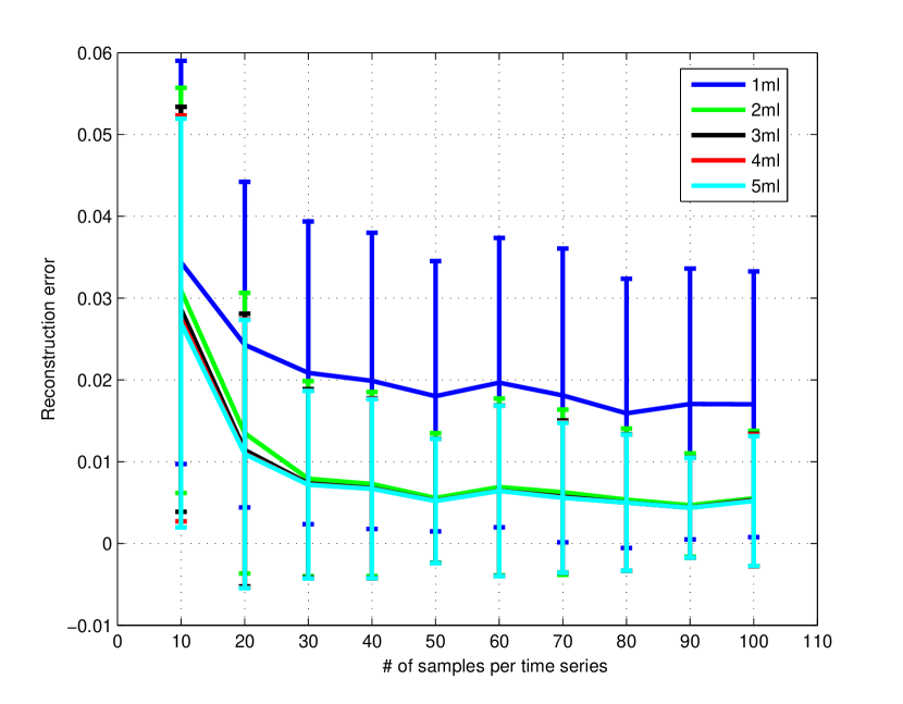
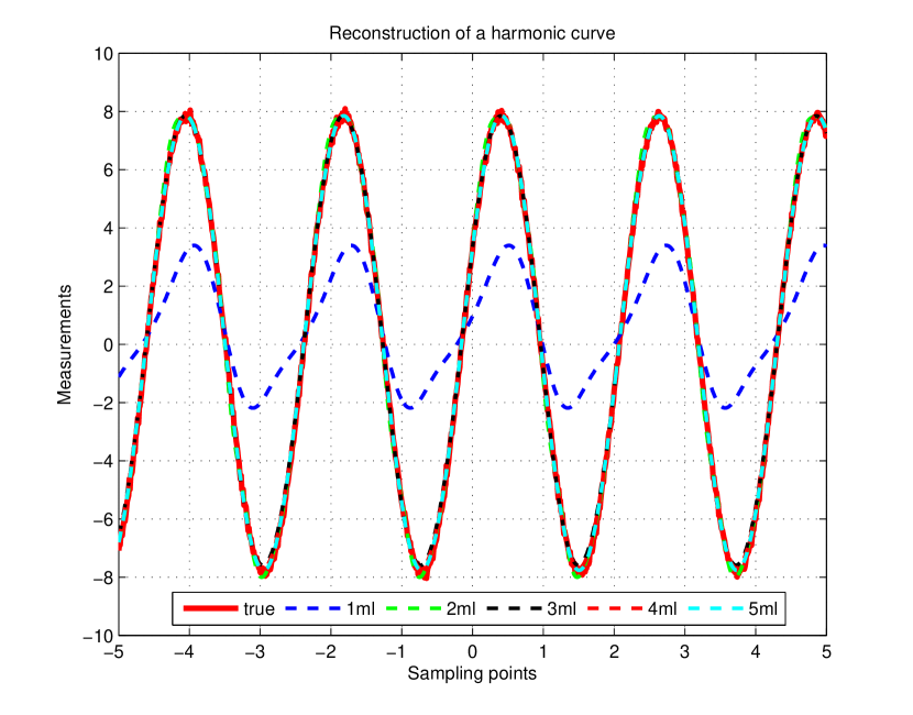
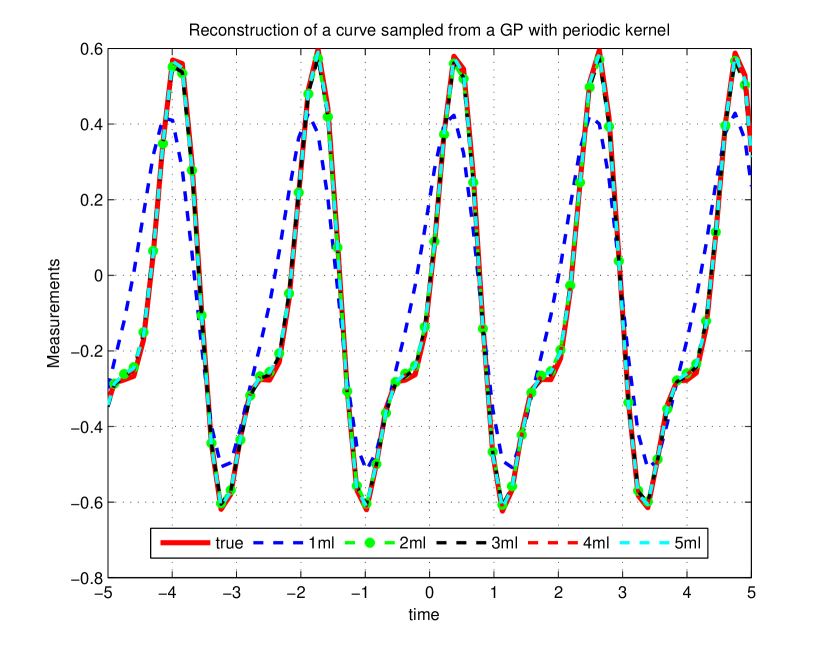
Figure 6.— Results for harmonic data (left column) and GP data (right column). Left: Accuracy (mean and standard deviation) versus the number of samples, where solid lines marked with $n$ml represent GP with marginal likelihood where $n$ denotes the number of iterations. The corresponding dotted lines marked $n$rss denote cross-validation results with $n$ iterations. Middle: Reconstruction error for the regression function versus the number of samples. Right: Reconstruction curve of GP in two specific runs using maximum likelihood with different number of iterations.

We generate two types of artificial data, referred to as harmonic data and GP data below. For the first, data is sampled from a simple harmonic function,

$$y\sim\mathcal{N}\left(a\sin(\omega x+\phi_{1})+b\cos(\omega x+\phi_{2}),\sigma^{2}\mathbb{I}\right)$$ (19)

where $a,b\sim\text{Uniform}(0,5)$, $\omega\sim\text{Uniform}(1,4)$, $\phi_{i}\sim\mathcal{N}(0,1)$ and the noise level $\sigma^{2}$ is set to be 0.1. Note that this is the model assumed by LS. For the second, data is sampled from a GP with periodic covariance function in Equation (8). We generate $\beta,\ell$ uniformly in $(0,3]$ and $(0,3]$ respectively and the noise level $\sigma^{2}$ is set to be 0.1. The period is drawn from a uniform distribution between $(0.5,2.5]$. For each type we generate data under the following configuration. We randomly sampled 50 time series each having 100 time samples in the interval $[-5,5]$. Then the comparison is performed using sub-samples with size increasing from 10 to 100. This is repeated ten times to generate means and standard deviations in the plots.

The setting of the algorithms is as follows: In our algorithm we only use one stage grid search. For our algorithm and LS, the lowest frequency $f_{\min}$ to be examined is the inverse of the span of the input data $1/(x_{\max}-x_{\min})=1/T$. The highest frequency $f_{\max}$ is twice the Nyquist frequency $f_{N}$, which we would obtain, if the data points were evenly spaced over the same span $T$, that is $f_{N}=N/(2T)$. We use an over-sample factor of 8, meaning that the range of frequencies is broken into even segments of $1/8T$. For PDM we set the frequency range to be $[0.02,5]$ with the frequency increments of 0.001 and the number of bins in the folded period is set to be 15.

For performance measures we consider both “accuracy” in identifying the period and the error of the regression function. For accuracy, we consider an algorithm to correctly find the period if its error is less than $1\%$ of the true period, i.e., $|\hat{p}-p|/p\leqslant 1\%$. Further experiments (not shown here) justify this approach by showing that the accuracies reported are not sensitive to the predefined error threshold.

The results, where our algorithm does not use the sampling and low rank approximations, are shown in Figure 6 and they support the following observations.

1. As expected, the top left plot shows that LS performs very well on the harmonic data and it outperforms both PDM and our algorithm. This means that if we know that the expected shape is sinusoidal, then LS is the best choice. This confirms the conclusion of other studies. For example, in the problem of detecting periodic genes from irregularly sampled gene expressions (Wentao et al., 2008; Glynn et al., 2006), the periodic time series of interest were exactly sine curves. In this case, studies showed that LS is the most effective comparing to several other statistical models.

2. On the other hand, the top right plot shows that our algorithm is significantly better than LS on the GP data showing that when the curves are non-sinusoidal the new model is indeed useful.

3. The two plots in top row together show that our algorithm performs significantly better than PDM on both types of data, especially when the number of samples is small.

4. The first two rows show the performance of the cyclic optimization procedure with 1-5 iterations. We clearly see that for these datasets there is little improvement beyond two iterations. The bottom row shows two examples of the learned regression curves using our method with different number of iterations. Although one iteration does find the correct period, the reconstruction curves are not accurate. However, here too, there is little improvement beyond two iterations. This shows that for the data tested here two iterations suffice for period estimation and for the regression problem.

5. The performance of marginal likelihood and cross validation is close, with marginal likelihood dominating on the harmonic data and doing slightly worse in GP data.

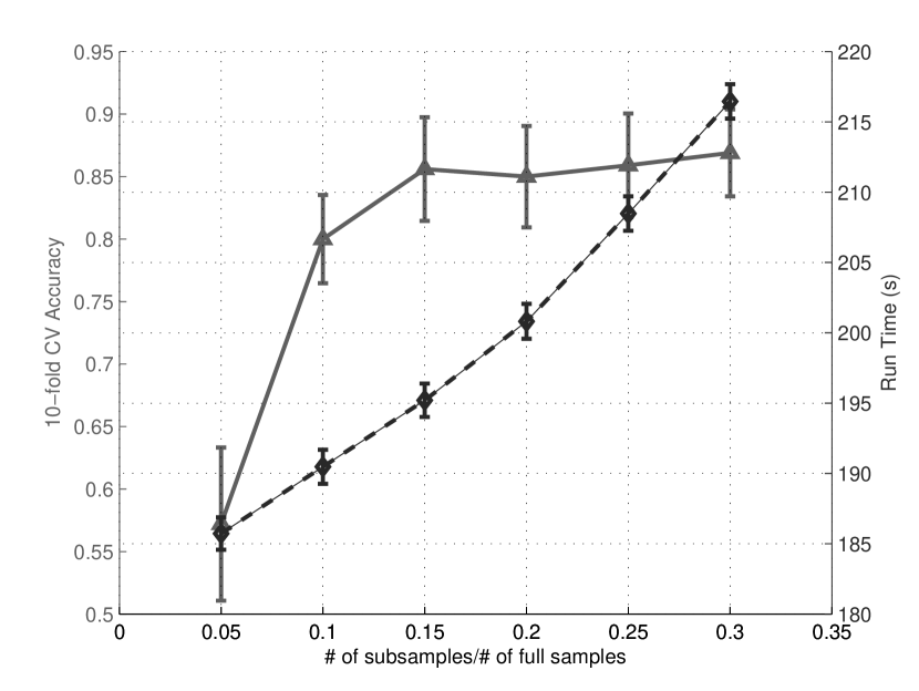
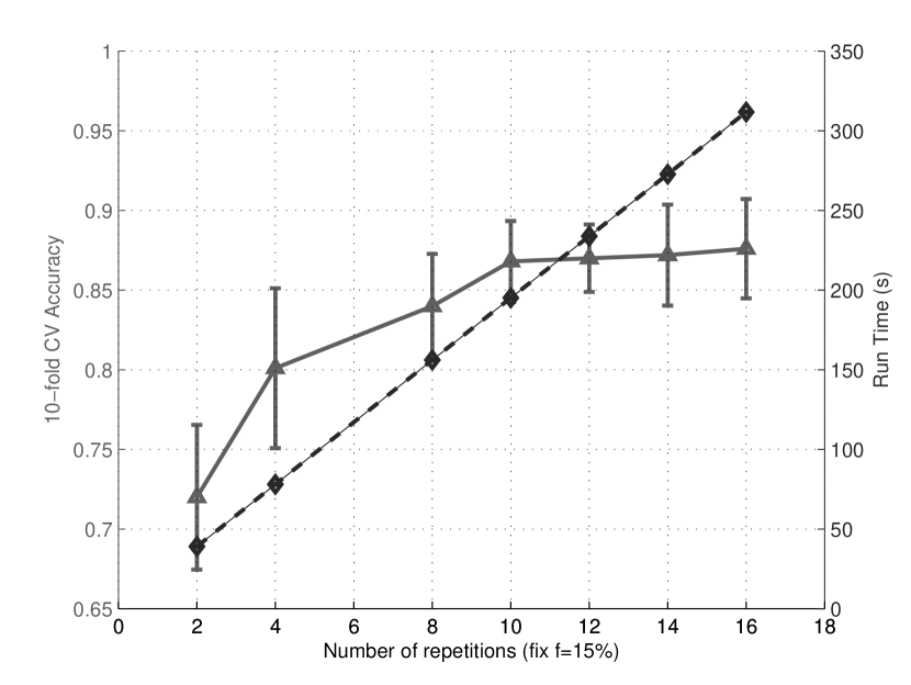
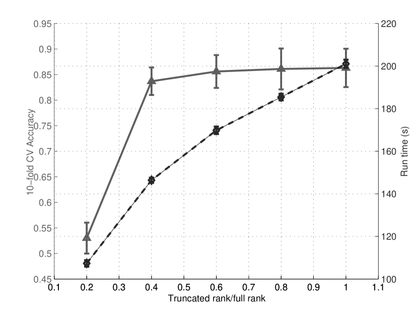
Figure 7.— Accuracy (solid line) and Run time (dash-line) of approximation methods as a function of their parameters. Left: sub-sampling ratio (with $R=10$). Middle: number of repetitions (with 15% sub-sampling). Right: rank in low rank approximation.

We next investigate the performance of the speedup techniques. For this we use GP data under the same configuration as the previous experiments. The experiment was repeated 10 times where in each round we generate 100 lightcurves each having 100 samples but generated from different $\theta$s. For the algorithm we used two iterations for cyclic optimization and varied the subsampling size, number of repetitions and rank of the approximation. Table 1 shows results with our chosen parameter setting using sampling rate of 15%, 10 repetitions, approximation rank $M=\lfloor\frac{N}{2}\rfloor$ and grid search threshold $\epsilon=0.005$. We can see that the subsampling technique saves over 60% percent of the run time while at the same time slightly increasing the accuracy. Low rank Cholesky approximation leads to an additional 15% decrease in run time, but gives slightly less good performance. Figure 7 plots the performance of the speedup methods under different parameter settings. The figure clearly shows that the chosen setting provides a good tradeoff in terms of performance vs. run time.

Table 1Comparison of GPs: Original, Subsampling and Subsampling plus low rank Cholesky update. Acc denotes accuracy and S/TS denotes the running time in seconds per time series.

	original	subsampling	sub + lowR
Acc	$0.831\pm 0.033$	$\mathbf{0.857\pm 0.038}$	$0.849\pm 0.028$
s/ts	$518.52\pm 121.49$	$197.59\pm 14.10$	$\mathbf{170.75\pm 17.93}$

4.2. Astrophysics Data

In this section, we estimate the periods of unfolded astrophysics time series from the OGLEII survey (Soszynski et al., 2003).

OGLE surveyed the sky over a number of years and has a huge number of light sources. The data we use here is a subset of OGLEII, containing a total of 14087 light curves of periodic variable stars that have previously been identified to be periodic (and thus their period is known) and to be members of one of 3 types: Cepheids, RR Lyrae, and Eclipsing Binary (illustrated in Figure 8).

We first explore, validate and develop our algorithm using a subset of OGLEII data and then apply the algorithm to the full OGLEII data except this development set. The OGLE subset is chosen to have 600 time series in total where each category is sampled according to its proportion in the full dataset.

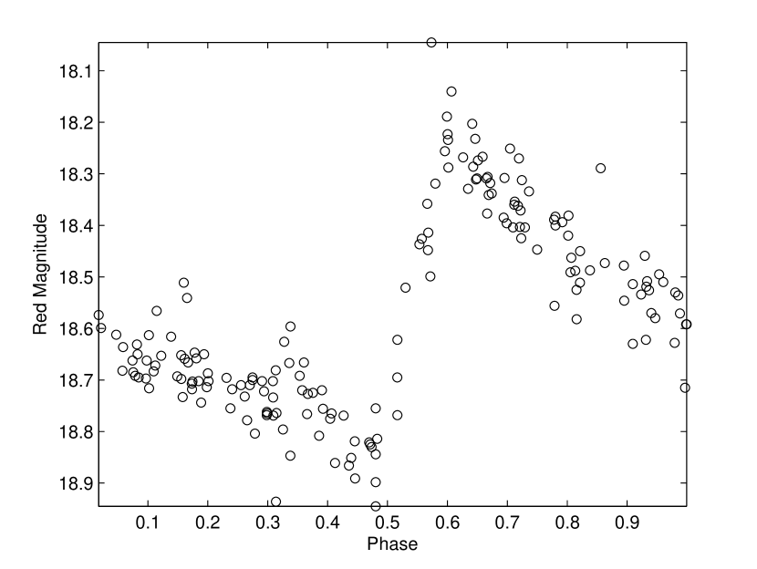
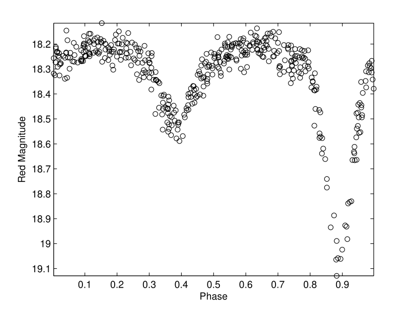
Figure 8.— Examples of light curves of periodic variable stars folded according to their period to highlight the periodic shape. Left: Cepheid, middle: RR Lyrae, right: Eclipsing Binary.

4.2.1 Evaluating the General GP Algorithm

The setting for our algorithm is as follows: The grid search ranges are chosen to be appropriate for the application using coarse grid of $[0.02,5]$ in the frequency domain with the increments of 0.001. The fine grid is a 0.001 neighborhood of the top frequencies each having 20 points with a step of 0.0001. We use $K=20$ top frequencies in step 9 of the algorithm and vary the number of iterations in a cyclic optimization. When using sub-sampling, we use 15% of the original time series, but restrict sample size to be between 30 and 40 samples. This guarantees that we do not use too small a sample and that complexity is not too high. For LS we use the same configuration as in the synthetic experiment. Results are shown in Table 2 and they mostly confirm our conclusions from the synthetic data. In particular, ML is slightly better than CV and subsampling yields a small improvement. In contrast with the artificial data, more iterations do provide a small improvement in performances and 5 iterations provide the best results in this experiment. Finally, we can also see that all of the GP variants outperform LS.

Table 2Comparisons of different GPs on OGLEII subset. gp-ml and gp-cv are GP with the ML and CV criteria. sgp-ml and sgp-cv are the corresponding subsampling versions. The first column denotes the number of iterations.

	gp-ml	gp-cv	sgp-ml	sgp-cv	ls
1itr acc	$0.7856$	$0.7769$	$0.7874$	0.7808	0.7333
2itr acc	$0.7892$	$0.7805$	$0.7910$	0.7818	-
3itr acc	$0.7928$	$0.7806$	$0.7964$	0.7845	-
4itr acc	$0.7946$	$0.7812$	$0.7982$	0.7875	-
5itr acc	$0.7964$	$0.7823$	$0.8000$	0.7906	-

Although this is an improvement over existing algorithms accuracy of 80% is still not satisfactory. As discussed by  Wachman (2009), one particularly challenging task is finding the true period of EB stars. The difficulty comes from the following two aspects. First, for a symmetric EB, the true period and half of the true period are not clearly distinguishable quantitatively. Secondly, methods that are better able to identify the true period of EBs are prone to find periods that are integer multiples of single bump stars like RRLs and Cepheids. On the other hand, methods that fold RRLs and Cepheids correctly often give “half” of the true period of EBs. In particular, the low performance of LS is due to the fact that it gives a half or otherwise wrong period for most EBs.

To illustrate the results Figure 9 shows the periods found by our method and by GP on 4 stars. The top row shows 2 cases where the GP method finds the correct period and LS finds half the period. The bottom row shows cases where LS identifies the correct period and the GP does not. In the example on the left the GP doubles the period. In the example on the right the GP identifies a different period from LS but given the spread in the correct period the period it uncovers is not unreasonable.

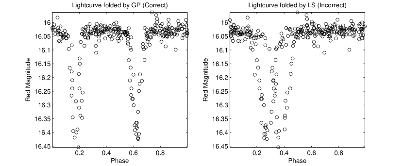
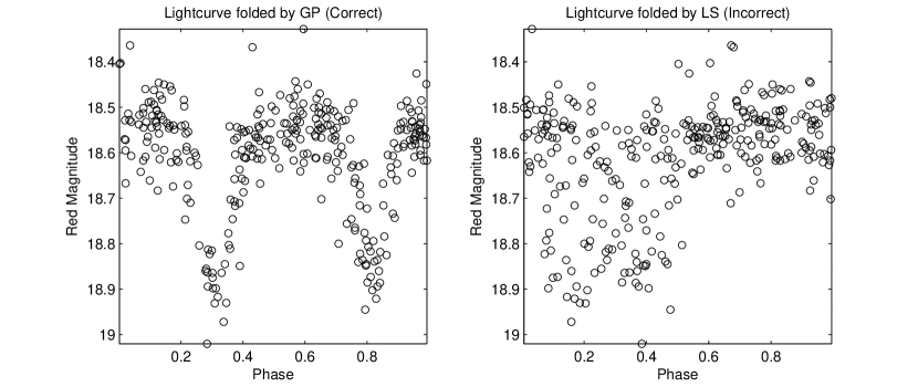
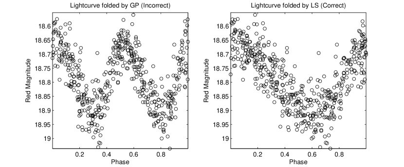
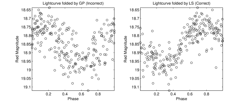
Figure 9.— Examples of light curves where GP and LS and identify different periods and one of them is correct. Each pair shows the time series folded by GP on the left and LS on the right. The top row shows cases where LS identifies half the period. The bottom row shows cases where GP identifies double the period or a different period.

4.2.2 Incorporating Domain Knowledge

We next show how this issue can be alleviated and the performance can be improved significantly using a learned probabilistic generative model. The methods developed are general and can be applied whenever such a model is available. As illustrated in Figure 8, our astrophysics knowledge suggests that different types of stars have different typical shift-invariant “shapes”. In addition, each class has more than one such shape and each individual star has some variation from the common shape. We use the Shift-invariant Grouped Mixed-effect Model (gmt) (Wang et al., 2010), which captures the common “shapes” via a mixture of Gaussian processes while at the same time allowing for individual variations. This model was previously developed to capture and aid in the classification of the astrophysics data. Once model parameters are learned we can calculate the likelihood of a light curve folded using a proposed period. Given the models, learned from a disjoint set of time series, for Cepheids, EBs and RRLs with parameter sets $\mathcal{M}_{i},i=\{C,E,R\}$, there are two perspectives on how they can be used:

Table 3Comparison of different regularization parameters on OGLEII subset using MAP.

$\gamma$	0	.1	.3	.5	.7	.9	1
acc	0.87027	0.85946	0.81802	0.81802	0.80901	0.80721	0.8

Model as Prior: The models can be used to induce an improper prior distribution (or alternatively a penalty function) on the period $p$. Given period $p$ and sample points $\bm{x}$ the prior is given by

$$\Pr(p)=\underset{i\in\{C,E,R\}}{\max}\left(\Pr(\bm{y}|\bm{x},p;\mathcal{M}_{i})\right)$$ (20)

where from the perspective of $\mathcal{M}_{i}$, $\bm{x}$ and corresponding points in $\bm{y}$ are interpreted as if they were sampled modulo $p$. Thus, combining this prior with the marginal likelihood, a Maximum A Posteriori (MAP) estimation can be obtained. Adding a regularization parameter $\gamma$ to obtain a tradeoff between the marginal likelihood and the improper prior we get our criterion:

$$\begin{split}\log\Pr(p|\bm{x},\bm{y};\mathcal{M})&=\gamma\log\Pr(\bm{y}|\bm{x},p;\mathcal{M})\\ &\quad+(1-\gamma)\log\Pr(p)\end{split}$$ (21)

where $\Pr(\bm{y}|\bm{x},p;\mathcal{M})$ is exactly as Equation (12) where the period portion of $\mathcal{M}$ is fixed to be $p$. When using this approach with our algorithm we use Equation (21) instead of Equation (12) as the score function in lines 5 and 13 of the algorithm. The results for different values of $\gamma$ (with subsampling and $5$ iterations) are shown in Table 3. The results show that gmt on its own ($\gamma=0$) is a good criterion for period finding. This is as one might expect because the OGLEII dataset includes only stars of the three types captured by gmt.

In this experiment, regularized versions do not improve the result of the gmt model. However, we believe that this will be the method of choice in other cases when the prior information is less strong. In particular, if the data includes unknown shapes that are not covered by the generative model then the prior on its own will fail. On the other hand when using Equation (21) with enough data the prior will be dominated by the likelihood term and therefore the correct period can be detected. In contrast, the filter method discussed next does not have such functionality.

Model as Filter: Our second approach uses the model as a post-processing filter and it is applicable to any method that scores different periods before picking the top scoring one as its estimate. For example, suppose we are given the top $K$ best periods $\{p_{i}\},i=1,\cdots,K$ found by LS, then we choose the one such that

$$p^{*}=\underset{i\in\{1,\cdots,K\}}{\text{argmax}}\left(\underset{j\in\{C,E,R\}}{\max}\left[\log\Pr(\bm{y}|\bm{x},p_{i};\mathcal{M}_{j})\right]\right).$$ (22)

Thus, when using the gmt as a filter, step 17 in our algorithm is changed to record the top $K$ frequencies from the last for loop, evaluate each one using the gmt model likelihood, and output the top scoring frequency.

Heuristic for Variable Periodic Stars: The two approaches above are general and can be used in any problem where a model is available. For the astrophysics problem we develop another heuristic that specifically addresses the half period problem of EBs. In particular, when using the filter method, instead of choosing the top $K$ periods, we double the selected periods, evaluate both the original and doubled periods $\{p_{i},2p_{i}\}$ using the gmt model, and choose the best one.

Results of experiments using the filter method with and without the domain specific heuristic are given in Table 4, based on the 5 iteration version of subsampling GP. The filter method significantly improve the performance of our algorithm showing its general applicability. The domain specific heuristic provides an additional improvement. For LS, the general filter method does not help but the domain specific heuristic significantly improves its performance. By analyzing the errors of both GP and LS, we found that their error regions are different. Therefore, we further propose a method that combines the two methods in the following way: pick the top $K$ periods found by both methods and evaluate the original and doubled periods using the gmt to select the best one. As Table 4 shows, the combination gives an additional 2% improvement on the OGLEII subset.

Table 4Comparisons of different algorithms on OGLEII subset using the GMT as a filter. Single denotes without the double period heuristic.

	original	single filter	filter
ls	0.7333	0.7243	0.9053
gp	0.8000	0.8829	0.9081
ls+gp	-	0.8811	0.9297

Table 5Comparisons of accuracies for full set of OGLEII.

	method in (Wachman, 2009)	ls-filter	gp-filter	gp-ls-filter
acc	0.8680	$0.8975\pm 0.04$	$0.8963\pm 0.03$	$\mathbf{0.9243\pm 0.03}$

4.2.3 Application

Finally, we apply our method using marginal likelihood with two level grid search, sub-sampling at 15%, 2 iterations, and filtering on the complete OGLEII data set with 13974 instances minus the development OGLEII subset. Note that the parameters of the algorithm, other than domain dependent heuristics, are chosen based on our results from the artificial data. The accuracy is reported using 10-fold cross validation under the following setting: the gmt is trained using the training set and we seek to find the periods for the stars in the test set. We compare our results to the best result from (Wachman, 2009) that used an improvement of LS, despite the fact that they filtered out 1719 difficult stars due to insufficient sampling points and noise. The results are shown in Table 5. We can see that our approach significantly outperforms existing methods on OGLEII.

5. Related Work

Period detection has been extensively studied in the literature and especially in astrophysics. The periodogram, as a tool for spectral analysis, dates back to the 19th century when Schuster applied it to the analysis of some data sets. The behavior of the periodogram in estimating frequency was discussed by Deeming (1975). The periodogram is defined as the modulus-squared of its discrete Fourier transform (Deeming, 1975). Lomb (1976) and Scargle (1982) introduced the so-called Lomb-Scargle (LS) Periodogram that was discussed above and which rates periods based on the sum-of-squares error of a sine wave at the given period. This method has been used in astrophysics (Cumming, 2004; Wachman, 2009) and has also been used in Bioinformatics (Glynn et al., 2006; Wentao et al., 2008). One can show that the LS periodogram is identical to the equation we would derive if we attempted to estimate the harmonic content of a data set at a specific frequency using the linear least-squares model (Scargle, 1982). This technique was originally named least-squares spectral analysis method Vaníček (1969). Many extensions of the LS periodogram exist in the literature (Bretthorst, 2001). Hall & Li (2006) proposed the periodogram for non-parametric regression models and discussed its statistical properties. This was later applied to the situation where the regression model is the superposition of functions with different period (Hall, 2008).

The other main approach uses least-squares estimates, equivalent to maximum likelihood methods under Gaussian noise assumption, using different choices of periodic regression models. This approach, using finite-parameter trigonometric series of different orders, has been explored by various authors (Hartley, 1949; Quinn & Thomson, 1991; Quinn & Fernandes, 1991; Quinn, 1999; Quinn & Hannan, 2001). Notice that if the order of the trigonometric series is high then this is very close to nonparametric methods (Hall, 2008).

Another intuition is to minimize some measure of dispersion of the data in phase space. Phase Dispersion Minimization (Stellingwerf, 1978), described above, performs a least squares fit to the mean curve defined by averaging points in bins. Lafler & Kinman (1965) described a procedure which involves trial-period folding followed by a minimization of the differences between observations of adjacent phases.

Other least squares methods use smoothing based on splines, robust splines, or variable-span smoothers. Craven & Wahba (1978) discussed the problem of smoothing periodic curve with spline functions in the regularization framework and invented the generalized cross-Validation (GCV) score to estimate the period of a variable star. Oh et al. (2002) extended it by substituting the smoothing splines with robust splines to alleviate the effects caused by outliers. Supersmoother, a variable-span smoother based on running linear smooths, is used for frequency estimation in (McDonald, 1986).

Several other approaches exist in the literature. Perhaps the most related work is (Hall et al., 2000) who studied nonparametric models for frequency estimation, including the Nadaraya-Watson estimator, and discussed their statistical properties. This was extended to perform inference for multi-period functions (Hall & Yin, 2003) and evolving periodic functions (Genton & Hall, 2007; Hall, 2008). Our work differs from (Hall et al., 2000) in three aspects: 1) the GP framework presented in this paper is more general in that one can plug in different periodic covariance functions for different prior assumptions; 2) we use marginal likelihood that can be interpreted to indicate how the data agrees with our prior belief; 3) we introduce mechanisms to overcome the computational complexity of period selection.

Other approaches include entropy minimization (Huijse et al., 2011), data compensated discrete Fourier transform (Ferraz-Mello, 1981), and Bayesian models (Gregory & Loredo, 1996; Scargle, 1998). Recently, Bayesian methods have also been applied to solve the frequency estimation problem, such as Bayesian binning for Poisson-regime (Gregory & Loredo, 1996) and Bayesian blocks (Scargle, 1998).

6. Conclusion

The paper introduces a nonparametric Bayesian approach for period estimation based on Gaussian process regression. We develop a model selection algorithm for GP regression that combines gradient based search and grid search, and incorporates several algorithmic improvements and approximations leading to a considerable decrease in run time. The algorithm performs significantly better than existing state of the art algorithms when the data is not sinusoidal. Further, we show how domain knowledge can be incorporated into our model as a prior or post-processing filter, and apply this idea in the astrophysics domain. Our algorithm delivers significantly higher accuracy than existing state of the art in estimating the periods of variable periodic stars.

An important direction for future work is to extend our model to develop a corresponding statistical test for periodicity, that is, to determine whether a time series is periodic. This will streamline the application of our algorithm to new astrophysics catalogs such as MACHO (Alcock et al., 1993) where both periodicity testing and period estimation are needed. Another important direction is establishing the theoretical properties of our method. Hall et al. (2000) provided the first-order properties of nonparametric estimators such that under mild regularity conditions, the estimator is consistent and asymptotically normally distributed. Our method differs in two ways: we use a GP regressor instead of Nadaraya-Watson estimator, and we choose the period that minimizes marginal likelihood rather than using a cross-validation estimate. Based on the well known connection between kernel regression and GP regression, we conjecture that similar results exist for the proposed method.

Appendix A Low rank approximation

In this appendix, we complete the details on how the first order approximation with low rank approximation can be achieved by a series of rank one updates/downdates of the Cholesky factors. As shown by Seeger (2007) each such update can be done in $\mathcal{O}(N^{2})$ using a series of Givens rotations.

It can be easily seen that $\widetilde{\bm{K}}$ is a real symmetric matrix. Denote its eigendecomposition as $\widetilde{\bm{K}}=\bm{U}\bm{\Lambda}\bm{U}^{T}$, then it can be written as the sum of a series of rank one components,

$$\widetilde{\bm{K}}=\sum_{i=1}^{N}\text{sgn}(\lambda_{i})\left(\sqrt{|\lambda_{i}|}\mathbf{u}_{i}\right)\left(\sqrt{|\lambda_{i}|}\mathbf{u}_{i}\right)^{T}$$ (A1)

where $\lambda_{i}$ is the $i$th eigenvalue and $\mathbf{u}_{i}$ is the corresponding eigenvector. Furthermore, we perform a low rank approximation to $\widetilde{\bm{K}}$ such that

$$\widetilde{\bm{K}}\approx\sum_{i=1}^{M}\text{sgn}(\lambda_{(i)})\left(\sqrt{|\lambda_{(i)}|}\mathbf{u}_{(i)}\right)\left(\sqrt{|\lambda_{(i)}|}\mathbf{u}_{(i)}\right)^{T}$$ (A2)

where $M<N$ is a predefined rank and $\lambda_{(i)}$ and $\mathbf{u}_{(i)}$ are the $i$th largest (in absolute value) eigenvalue and its corresponding eigenvector. Therefore we have,

$$\bm{K}_{w_{1}}\approx\bm{L}\bm{L}^{T}+\sum_{i=1}^{M}\text{sgn}(\lambda_{(i)})((\Delta w)^{1/2}\bm{\ell}_{i})((\Delta w)^{1/2}\bm{\ell}_{i})^{T}$$ (A3)

where $\bm{\ell}_{i}=\sqrt{|\lambda_{(i)}|}\mathbf{u}_{(i)}$. We can see that the complexity for calculating the Cholesky factor of $\bm{K}_{w_{1}}$ becomes $\mathcal{O}(MN^{2})$. Therefore, we can choose an $\epsilon$-net $\mathcal{E}$ of the fine grid such that $\forall w\in\mathcal{F},\sup_{v\in\mathcal{E}}|w-v|<\epsilon$, perform the exact Cholesky decomposition directly only on the $\epsilon$-net, and use the approximation on the other frequencies. In this way we reduce the complexity from $\mathcal{O}(|\mathcal{F}|N^{3})$ to $\mathcal{O}(|\mathcal{E}|N^{3}+|\mathcal{F}|MN^{2})$.

References

- Alcock et al. (1993) Alcock, C., et al. 1993, in Astronomical Society of the Pacific Conference Series, Vol. 43, Sky Surveys. Protostars to Protogalaxies, ed. B. T. Soifer, 291–296
- Bishop (2006) Bishop, C. 2006, Pattern recognition and machine learning, Vol. 4 (Springer New York)
- Bretthorst (2001) Bretthorst, G. 2001, in Bayesian Inference and Maximum Entropy Methods in Science and Engineering, Vol. 568, 246–251
- Craven & Wahba (1978) Craven, P., & Wahba, G. 1978, Numerische Mathematik, 31, 377
- Cumming (2004) Cumming, A. 2004, Monthly Notices of the Royal Astronomical Society, 354, 1165
- Deeming (1975) Deeming, T. 1975, Astrophysics and Space Science, 36, 137
- Ferraz-Mello (1981) Ferraz-Mello, S. 1981, The Astronomical Journal, 86, 619
- Genton & Hall (2007) Genton, M., & Hall, P. 2007, Journal of the Royal Statistical Society: Series B (Statistical Methodology), 69, 643
- Glynn et al. (2006) Glynn, E., Chen, J., & Mushegian, A. 2006, Bioinformatics, 22, 310
- Gregory & Loredo (1996) Gregory, P., & Loredo, T. 1996, The Astrophysical Journal, 473, 1059
- Hall (2008) Hall, P. 2008, COMPSTAT 2008, 3
- Hall & Li (2006) Hall, P., & Li, M. 2006, Biometrika, 93, 411
- Hall et al. (2000) Hall, P., Reimann, J., & Rice, J. 2000, Biometrika, 87, 545
- Hall & Yin (2003) Hall, P., & Yin, J. 2003, Journal of the Royal Statistical Society: Series B (Statistical Methodology), 65, 869
- Hartley (1949) Hartley, H. 1949, Biometrika, 36, 194
- Huijse et al. (2011) Huijse, P., Estevez, P. A., Zegers, P., Principe, J. C., & Protopapas, P. 2011, IEEE Signal Processing Letters, 18, 371
- Lafler & Kinman (1965) Lafler, J., & Kinman, T. 1965, The Astrophysical Journal Supplement Series, 11, 216
- Lomb (1976) Lomb, N. 1976, Astrophysics and space science, 39, 447
- McDonald (1986) McDonald, J. 1986, SIAM Journal on Scientific and Statistical Computing, 7, 665
- Oh et al. (2002) Oh, H., Nychka, D., Brown, T., & Charbonneau, P. 2002, Period analysis of variable stars by a robust method
- Petit (1987) Petit, M. 1987, Variable stars, ed. Petit, M.
- Protopapas et al. (2005) Protopapas, P., Jimenez, R., & Alcock, C. 2005, Monthly Notices of the Royal Astronomical Society, 362, 460
- Quinn (1999) Quinn, B. 1999, Biometrika, 86, 213
- Quinn & Fernandes (1991) Quinn, B., & Fernandes, J. 1991, Biometrika, 78, 489
- Quinn & Hannan (2001) Quinn, B., & Hannan, E. 2001, The estimation and tracking of frequency (Cambridge Univ Pr)
- Quinn & Thomson (1991) Quinn, B., & Thomson, P. 1991, Biometrika, 78, 65
- Rasmussen & Nickisch (2010) Rasmussen, C., & Nickisch, H. 2010, Journal of Machine Learning Research, 11, 3011
- Rasmussen & Williams (2005) Rasmussen, C., & Williams, C. 2005, Gaussian Processes for Machine Learning (The MIT Press)
- Reimann (1994) Reimann, J. 1994, PhD thesis, UC Berkeley
- Scargle (1982) Scargle, J. 1982, The Astrophysical Journal, 263, 835
- Scargle (1998) —. 1998, The Astrophysical Journal, 504, 405
- Seeger (2007) Seeger, M. 2007, University of California at Berkeley, Tech. Rep
- Soszynski et al. (2003) Soszynski, I., Udalski, A., & Szymanski, M. 2003, Acta Astronomica, 53, 93
- Stellingwerf (1978) Stellingwerf, R. 1978, The Astrophysical Journal, 224, 953
- Vaníček (1969) Vaníček, P. 1969, Astrophysics and Space Science, 4, 387
- Wachman (2009) Wachman, G. 2009, PhD thesis, Tufts University
- Wang et al. (2010) Wang, Y., Khardon, R., & Protopapas, P. 2010, Machine Learning and Knowledge Discovery in Databases, 418
- Wentao et al. (2008) Wentao, Z., Kwadwo, A., Erchin, S., et al. 2008, EURASIP Journal on Bioinformatics and Systems Biology, 2008