Experimental estimation of the dimension of classical and quantum systems

Abstract

An overwhelming majority of experiments in classical and quantum physics make a priori assumptions about the dimension of the system under consideration. However, would it be possible to assess the dimension of a completely unknown system only from the results of measurements performed on it, without any extra assumption? The concept of a dimension witness brunner ; perezgarcia ; wehner ; perez ; gbha answers this question, as it allows one to bound the dimension of an unknown classical or quantum system in a device-independent manner, that is, only from the statistics of measurements performed on it. Here, we report on the experimental demonstration of dimension witnesses in a prepare and measure scenario gbha . We use pairs of photons entangled in both polarization and orbital angular momentum molina-terriza2007 ; mair2001 to generate ensembles of classical and quantum states of dimensions up to 4. We then use a dimension witness to certify their dimensionality as well as their quantum nature. Our results open new avenues for the device-independent estimation of unknown quantum systems mayers ; bardyn ; bancal ; rabelo and for applications in quantum information science marcin ; guo .

Any physical theory aims at providing an explanation for the results of measurements performed on a system under different conditions. Given a system, one makes some general and plausible assumptions about its behavior, builds a theory compatible with these assumptions and tests its predictive power under different experimental configurations. The dimension of the system, that is, the number of relevant and independent degrees of freedom needed to describe it, is in general an a priori parameter and represents one of these initial assumptions. In general, the failure of a theoretical model in predicting experimental data does not necessarily imply that the assumption on the dimensionality is incorrect, as there might exist a different model in a space of the same dimension able to reproduce the observed data.

A natural question is whether this approach can be reversed and whether the dimension of an unknown system, classical or quantum, can be estimated experimentally. Clearly, the best one can hope for is to provide lower bounds on this unknown dimension. Indeed, one can never exclude that more degrees of freedom are necessary to describe the system in more complex experimental arrangements. The goal, then, is to obtain a lower bound on the dimension of the unknown system from the observed measurement data without making any assumption about the detailed functioning of the devices used in the experiment. Besides its fundamental interest, estimating the dimension of an unknown quantum system is also relevant from the perspective of quantum information, where the Hilbert space dimension is considered as a resource (see, e.g., lanyon ). For instance, the optimal quantum realization of some protocols, e.g. bit commitment, requires systems of a minimal dimension BC . Moreover, the dimension of quantum systems plays a crucial role in security proofs of standard quantum key distribution schemes that become insecure if the dimension is higher than assumed acingisin .

The concept of a dimension witness allows one to establish lower bounds on the dimension of an unknown system in a device-independent way, that is, only from the collected measurement statistics. It was first introduced for quantum systems in connection with Bell inequalities in brunner , and further developed in perezgarcia ; vertesi1 ; vertesi2 ; vertesi4 ; junge ; briet ; junge2 . Other techniques to estimate the dimension have been developed in scenarios involving random access codes wehner , or the time evolution of a quantum observable perez .

More recently, a general framework for the study of this question has been proposed in gbha . In this approach, dimension witnesses are defined in a prepare and measure scenario where an unknown system is subject to different preparations and measurements. One of the advantages of this approach is its simplicity from an experimental viewpoint when compared to previous proposals. The considered scenario consists of two devices (see Fig. 1), the state preparator and the measurement device. These devices are seen as black boxes, as no assumptions are made on their functioning. The state preparator prepares upon request a state. The box features $N$ buttons which label the prepared state; when pressing button $x$, the box emits a state $\rho_{x}$, where $x\in\{1,...,n\}$. The prepared state is then sent to the measurement device. The measurement box performs a measurement $y\in\{1,...,m\}$ on the state, delivering outcome $b\in\{1,...,k\}$. The experiment is thus described by the probability distribution $P(b|x,y)$, giving the probability of obtaining outcome $b$ when measurement $y$ is performed on the prepared state $\rho_{x}$. The goal is to estimate the minimal dimension that the ensemble $\left\{\rho_{x}\right\}$ must have to be able to describe the observed statistics. Moreover, for a fixed dimension, we also aim at distinguishing sets of probabilities $P(b|x,y)$ that can be obtained from ensembles of quantum states, but not from ensembles of classical states. This allows one to guarantee the quantum nature of an ensemble of states under the assumption that the dimensionality is bounded.

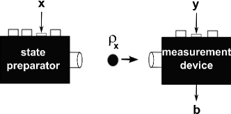
Figure 1: Sketch of a device-independent test of the dimension of an ensemble of quantum states. Our scenario features two black boxes: a state preparator, which generates one of $n$ possible states on demand, and a measurement device which performs one of $m$ possible measurements on the state generated.

Formally, a probability distribution $P(b|x,y)$ admits a $d$-dimensional representation if it can be written in the form

$$P(b|x,y)=\textrm{tr}(\rho_{x}M_{b}^{y}),$$ (1)

for some state $\rho_{x}$ and operator $M_{b}^{y}$ acting on $\mathbb{C}^{d}$. We then say that $P(b|x,y)$ has a classical $d$-dimensional representation if any state of the ensemble $\left\{\rho_{x}\right\}$ is a classical state of dimension $d$, i.e., a probability distribution over classical dits (or equivalently, all the states of the ensemble commute).

A dimension witness for classical (quantum) systems of dimension $d$ is defined by a linear combination of the observed probabilities $P(b|x,y)$, defined by a tensor of real coefficients $D_{b,x,y}$, such that

$$\sum_{b,x,y}D_{b,x,y}P(b|x,y)\leq w_{d}$$ (2)

for all probabilities with a $d$-dimensional representation, while this bound can be violated by a set of probabilities whose representation has a dimension strictly larger than $d$. A family of dimension witnesses $I_{N}$ was introduced recently  gbha in a scenario consisting of $N$ possible preparations and $N-1$ measurements with only two possible outcomes, labeled by $b=\pm 1$. Here we shall focus on one of these witnesses, namely

$$I_{4} \equiv E_{11}+E_{12}+E_{13}$$ (3)

$$+ E_{21}+E_{22}-E_{23}$$

$$+ E_{31}-E_{32}$$

$$- E_{41},$$

where $E_{xy}=P(b=+1|x,y)-P(b=+1|x,y)$. Witness $I_{4}$ features four preparations and three measurements. It can distinguish ensembles of classical and quantum states of dimensions up to $d=4$. All the relevant bounds are summarized in Table 1.

	$C_{2}$ (bit)	$Q_{2}$ (qubit)	$C_{3}$ (trit)	$Q_{3}$ (qutrit)	$C_{4}$ (quart)
$I_{4}$	5	6	7	7.97	9

Table 1: Classical and quantum bounds for the dimension witnesses $I_{4}$. The maximal possible value of $I_{4}$ for classical systems of dimension $d$ is denoted $C_{d}$, while the maximum possible value for quantum systems of dimension $d$ is denoted $Q_{d}$. The witness can be used to discriminate ensembles of classical and quantum states of dimension up to $d=4$. Note that for a given value of the dimension of the system, the witness can be used to certify its quantum nature.

In order to test this witness experimentally, we must generate classical and quantum states of dimension 2 (bits and qubits, respectively), classical and quantum states of dimension 3 (trits and qutrits), and classical states of dimension 4 (quarts). To do so we exploit the angular momentum of photons molina-terriza2007 ; mair2001 . The total angular momentum contains a spin contribution associated with the polarization, and an orbital contribution associated with the spatial shape of the light intensity and its phase. Within the paraxial regime, both contributions can be measured and manipulated independently. The polarization of photons can be described in a $2$-dimensional Hilbert space, as any polarization state can be described by a weighted superposition of two orthogonal polarization states (e.g., horizontal and vertical). The spatial degree of freedom of light lives in an infinite-dimensional Hilbert space, as any spatial waveform can be described in terms of a weighted superposition of modes that span an infinite-dimensional basis molina-terriza2002 . Paraxial Laguerre-Gaussian (LG) modes constitute one of these bases. LG beams are characterized by two integer indices, $p$ and $m$. The index $m$ determines the azimuthal phase dependence of the mode, which is of the form $\sim\exp\left(im\varphi\right)$, where $\varphi$ is the azimuthal angle in the cylindrical coordinates. LG laser beams carry a well-defined orbital angular momentum (OAM) of $m\hbar$ per photon that is associated with their spiral wavefronts allen1992 .

Our state preparator employs a source based on spontaneous parametric down-conversion (SPDC) that generates pairs of photons (signal and idler) entangled in both polarization and OAM. By performing a projective measurement on one photon of the pair (idler), we prepare its twin photon (signal) in a well-defined state. A given measurement outcome on the first photon (idler) corresponds to a given preparation for the second photon (signal), which represents the mediating particle of Fig. 1.

We use the state preparator to generate ensembles of states of dimension up to 4: two degrees of freedom are encoded in their polarization (horizontal or vertical) and two degrees of freedom are encoded in their OAM ($m=+1$ or $m=-1$). For the case of qubit preparations, the four states $|\phi_{x}\rangle$ ($x=1...4$) are enconded in the polarization only and have the same OAM of $m=+1$ (see the upper left part of Fig. 2). An analogous procedure is used to prepare a qutrit state, however, now state $|\phi_{3}\rangle$ carries OAM of $m=-1$, thus adding one dimension. The quart state is prepared by flipping the OAM of state $|\phi_{4}\rangle$. In this way we generate a 4-dimensional Hilbert, spanned by the orthogonal vectors $\left\{|H,+1\rangle,|H,-1\rangle,|V,+1\rangle,\rm{and}|V,-1\rangle\right\}$, where $|H,\pm 1\rangle$ and $|V,\pm 1\rangle$ stand for a horizontally or vertically polarized photon with OAM equal to $m=\pm 1$, respectively.

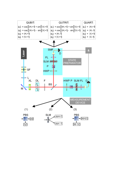
Figure 2: Experimental setup of the dimension witness. The upper part depicts the individual states $|\phi_{x}\rangle$ ($x=1...4$) prepared by the state preparator. The lower part illustrates the measurements performed by the measurement device. SF - spatial filter; L - lens; M - mirror; XL - nonlinear crystal; DL - delay line; F - 5-nm bandpass filter; BS - beamsplitter; HWP - half-wave plate; P - polarizer; SLM - spatial light modulator; PBS - polarizing beamsplitter; FL - Fourier-transform lens; SMF - single-mode fiber; D - single-photon counting detector; & - coincidence electronics.

To implement continuous transition from quantum to classical states, a polarization-dependent temporal delay between the two photons of an entangled pair is introduced. If the temporal delay between the photons exceeds their correlation time, the coherence is lost, i.e., the off-diagonal terms of the state in the ensemble go to zero (see Appendix).

Finally, the measurement device simply performs measurements on the second (signal) photon.

The experimental setup is shown in Fig. 2. The second harmonic (Inspire Blue, Spectra Physics/Radiantis) at a wavelength of 405 nm of a Ti:saphire laser in the picosecond regime (Mira, Coherent) is shaped by a spatial filter and focused into a 1.5-mm thick crystal of beta-barium borate (BBO), where SPDC takes place. The nonlinear crystal is cut for collinear type-II down-conversion so that the generated photons have orthogonal polarizations. Before splitting the photon pairs towards the state preparator and measurement device, the polarization-dependent temporal delay $\tau$ is introduced. The delay line (DL) consists of two quartz prisms whose mutual position determines the difference between the propagation times of photons with different polarizations.

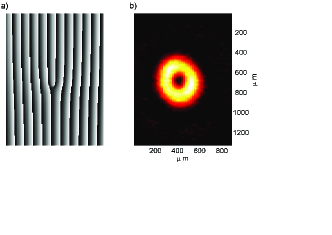
Figure 3: a) Computer generated hologram used to detect a LG beam with $m=+1$. b) CCD camera photograph of the generated LG mode when the hologram is illuminated by a Gaussian beam.

The measurement setup consists of a half-wave plate (HWP), polarizer (P), spatial-light modulator (SLM) and a Fourier-transform lens (FL). The half-wave plate and polarizer project the incoming idler photon into the desired polarization state. The desired OAM state is selected by the spatial light modulator. If the nonlinear crystal is pumped by the fundamental LG beam LG₀₀, about 15% of the entangled photons are generated in the LG mode with $m=\pm 1$ silvana . The OAM is conserved langford2004 ; molina-terriza2004 ; osorio2008 (see Appendix for more details), i.e., if the signal photon has $m=+1$, the idler must have $m=-1$ and vice versa. The SLM encodes computer-generated holograms that transform the $m=+1$ state or $m=-1$ state into the fundamental LG state LG₀₀ molina-terriza2007 that is coupled into a single-mode fiber (SMF). In this way, only a photon having a correct combination of its OAM with a corresponding hologram placed at the SLM is successfully coupled in the fiber and results in a subsequent click at the detector. Figure 3 a) shows a computer-generated hologram to measure an $m=+1$ state and Fig. 3 b) shows a picture of the LG mode taken by a CCD camera when this hologram is illuminated by a Gaussian beam.

When the polarizers in both arms are set to $+45$ degrees, a Hong-Ou-Mandel dip HOM of visibility above 95% is measured (see Fig. 4 a)). The center of the dip corresponds to the pure state generation when the qubit and qutrit states are prepared depending on their OAM. On the right-hand side, on the shoulder of the dip, the superposition is lost and the qubit and qutrit are converted to a classical bit and trit, respectively. The purity of the state is given by Eq. 8 that can be found in Appendix with more details.

To find the correct position of the hologram on the SLM, the center of the hologram must exactly coincide with the center of the down-converted beam. To overlap them perfectly, first the signal hologram is set to detect photons with $m=+1$ and the idler hologram is set to detect $m=0$. Then signal holograms with different central positions of the vortex are scanned across the SLM. Since the down-converted photons are generated with $m=\pm 1$, a minimum of coincident counts between $m=+1$ and $m=0$ tells us the correct position of the signal hologram (see Fig. 4 b)). Now with the signal hologram fixed, the idler hologram set to $m=-1$ is scanned to find a maximum number of coincidences. With both holograms in the correct place, the dimension witness is measured.

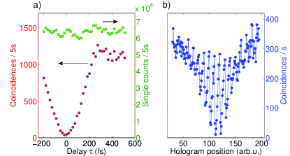
Figure 4: a) The Hong-Ou-Mandel dip shows the transition from a pure entangled state to a mixed state. The pure state is used to prepare a quantum superposition of $|H\rangle$ and $|V\rangle$, whereas the mixed state is used to prepare statistical mixtures of $|H\rangle$ and $|V\rangle$. b) Two-dimensional scan of the hologram position in the signal beam. Signal hologram is set to $m=+1$ and idler hologram is set to $m=0$. Disappearance of coincidences asserts the correct position of the hologram was found in order to detect signal photons with OAM $m=+1$.

First, the qubit ensemble is generated. We sequentially prepare the four qubit states $|\phi_{x}\rangle$ of Fig. 2 and perform the three desired measurements. The first measurement $y=1$ assigns dichotomic measurement results of $b=+1$ and $b=-1$ to horizontally and vertically polarized photons, respectively. The second measurement $y=2$ assigns $b=+1$ and $b=-1$ to OAM values of $m=+1$ and $m=-1$, respectively. And the third measurement $y=3$ assigns $b=+1$ and $b=-1$ to photons polarized at $+45^{o}$ and $-45^{o}$. The maximum theoretical value of the witness $I_{4}$ of Eq. 3 for this ensemble of states and this set of measurements is 5.83 (see Appendix). The experimentally measured witness reaches $I_{4}=5.66\pm 0.15$. This clearly demonstrates the quantum nature of our 2-dimensional system, since classical bits always satisfy $I_{4}\leq 5$.

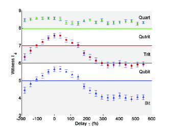
Figure 5: Dimension witness $I_{4}$ for qubit (blue triangles), qutrit (red circles) and quart (green diamonds) as a function of temporal delay $\tau$. For delays $\tau>255$ fs, coherence is lost and quantum superpositions turn into statistical mixtures, i.e., classical states. The maximum violations for qubit, qutrit and quart are $5.66\pm 0.15$, $7.57\pm 0.13$, and $8.57\pm 0.06$, respectively, which are close to the corresponding theoretical bounds, given in Table 1, which are represented here by the horizontal lines.

Now a variable temporal delay $\tau$ is introduced between the horizontal and vertical polarizations, and the value of the witness decreases below 5, leveling off at $\tau\approx 255$ fs that corresponds to the end of the Hong-Ou-Mandel dip, as expected (see blue triangles of Fig. 5). Thus our qubit is now converted into a classical bit.

If the OAM of state $|\phi_{3}\rangle$ is flipped, a qutrit is prepared and the dimension witness is measured. For a zero delay $\tau$, the value of the witness reaches $I_{4}=7.57\pm 0.13$, certifying the presence of a (at least) 3-dimensional quantum system. Here the maximum theoretical value for this ensemble of states and this set of measurements is $5+2\sqrt{2}\sim 7.83$ (see Appendix).

When the delay line is scanned, the values of the witness drop below 7, but in a certain range of $\tau$ they remain above the qubit bound of 6, testifying that at least three dimensions are present (see red circles of Fig. 5). In the classical limit of large delays, the witness values are still larger then the bound of $I_{4}=5$ for bits.

Finally, we prepare classical 4-dimensional systems, i.e. quarts. Now the first measurement $y=1$ assigns the dichotomic value of $b=+1$ to horizontally polarized photons of $m=\pm 1$ and to vertically polarized photons of $m=+1$, and $b=-1$ corresponds to vertically polarized photons with $m=-1$; the second measurement $y=2$ assigns $b=+1$ and $b=-1$ to horizontally and vertically polarized photons, respectively; and the third measurement $y=3$ assigns $b=+1$ and $b=-1$ to OAM values of $m=+1$ and $m=-1$, respectively. All the correlation coefficients should add up and should be equal to 1. The obtained value is $I_{4}=8.57\pm 0.06$, which violates the qutrit threshold by more than 10 standard deviations. In this case, the values of the witness remain constant and are independent of the temporal delay $\tau$. Indeed this is because the state is classical (a statistical mixture of orthogonal quantum states) and no superposition is present (see green diamonds of Fig. 5).

To conclude, we have demonstrated how the dimension of classical and quantum systems can be bounded only from experimental measurement results without any extra assumption on the devices used in the experiment. Dimension witnesses represent an example of a device-independent estimation technique, in which relevant information about an unknown system is obtained solely from the measurement data. Device-independent techniques (see also Refs. mayers ; bardyn ; bancal ; rabelo ) provide an alternative and robust approach to the estimation of quantum systems, especially when compared to most of the existing estimation techniques, such as quantum tomography, which crucially rely on some assumptions about the measured system, e.g., its Hilbert space dimension, that may be questionable in complex setups. Our work demonstrates how the device-independent approach can be employed to experimentally estimate the dimension of an unknown system.

I Appendix

In order to generate photons in the multidimensional Hilbert space defined by the angular momentum of light, and at the same time to be able to modify the dimension and the properties of the corresponding quantum states, we generate photon pairs entangled in the polarization and spatial degrees of freedom mair2001 .

If the beam sizes of the pump beam and those of the collection systems of the down-converted photons are large enough, we can neglect the effects of the Poynting-vector walk-off that takes place in a birefringent medium molina-terriza2007 . In this case, the generated paired photons are found to be embedded into LG modes with opposite winding numbers $m_{s}=-m_{i}$, where $m_{s,i}\hbar$ refers to the OAM of the signal and idler photons, respectively. After the down-conversion stage, a beam splitter is used to separate the signal and idler photons. If the optical system selects only the modes with $m_{s,i}=\pm 1$, the quantum state of the photon pairs can be written as

$$\Psi = \frac{1}{\sqrt{2}}\int d\Omega$$ (4)

$$\times \left\{f\left(\Omega\right)\left[|\Omega,H,+1\rangle_{1}|\Omega,V,-1\rangle_{2}\right.\right.$$

$$\qquad\left.+|\Omega,H,-1\rangle_{1}|\Omega,V,+1\rangle_{2}\right]$$

$$+ f\left(-\Omega\right)\left[|\Omega,V,+1\rangle_{1}|\Omega,H,-1\rangle_{2}\right.$$

$$\qquad\left.\left.+|\Omega,V,-1\rangle_{1}|\Omega,H,+1\rangle_{2}\right]\right\}.$$

The signal photon has frequency $\omega_{s}=\omega_{0}+\Omega$, and the idler photon has frequency $\omega_{i}=\omega_{0}-\Omega$, where $\omega_{0}$ is the central frequency of the down-converted photons and $\Omega$ is the frequency deviation from the central frequency. The function $f$ reads

$$f(\Omega)=\frac{DL}{2\pi}\text{sinc}\left(\frac{D\Omega L}{2}\right)\exp\left(i\frac{D\Omega L}{2}\right),$$ (5)

where $L$ is the crystal length, and $D=1/v_{s}-1/v_{i}$ is the difference of inverse group velocities ($v_{s,i}$) of the signal and idler photons.

The signal and idler photons are entangled in the polarization and spatial degrees of freedom. On the other hand, the frequency properties of entangled two-photon states cannot be neglected even when the entanglement resides in the other degrees of freedom. In most experiments, the entangled states take advantage of only a portion of the total two-photon quantum state and the generation of high-quality entanglement requires the suppression of any frequency “which-path” information that would otherwise degrade the degree of entanglement. Notwithstanding, here we use the presence of frequency “which-path” information to tailor the quantum nature of ensembles of signal photons.

We introduce a temporal delay $\tau$ between the orthogonally polarized signal and idler photons before they are separated at the beam splitter. In the idler path, a polarizer rotated by an angle $\varphi$, is placed, followed by a spatial light modulator which in combination with a single mode fiber selects idler photons in a LG mode with a winding number $m=\pm 1$. Thanks to the angular momentum correlations between signal and idler photons, the detection of an idler photon with horizontal or vertical polarization ($\varphi=0^{o}$) and with a spatial shape given by a LG mode with index $m=\pm 1$, projects the signal photon into the orthogonal polarization and a LG mode with index $m=\mp 1$. When the polarizer projects the idler photon in a weighted combination of the two orthogonal polarizations ($\varphi\neq 0^{o}$), the resulting quantum state of the signal photon depends on the delay $\tau$.

The Hilbert space of signal photons, defined by the angular momentum (i.e., polarization and orbital angular momentum), is spanned by vectors $\left\{|H,+1\rangle,|H,-1\rangle,|V,+1\rangle,{\rm and}|V,-1\rangle\right\}$. After tracing out the frequency degree of freedom, the quantum state of signal photons is given by the density matrix

$$\rho_{x}=\left(\begin{array}[]{cccc}\alpha\cos^{2}\varphi&0&\alpha\gamma(\tau)\sin 2\varphi/2&0\\ 0&(1-\alpha)\cos^{2}\varphi&0&(1-\alpha)\gamma(\tau)\sin 2\varphi/2\\ \alpha\gamma^{*}(\tau)\sin 2\varphi/2&0&\alpha\sin^{2}\varphi&0\\ 0&(1-\alpha)\gamma^{*}(\tau)\sin 2\varphi/2&0&(1-\alpha)\sin^{2}\varphi,\\ \end{array}\right),$$ (6)

where $\alpha=1$ if the idler photons is projected into a mode with $m=-1$, and $\alpha=0$ if the idler photon is projected into a mode with $m=1$.

The parameter $\gamma(\tau)$, which fulfills the condition $|\gamma(\tau)|\leq 1$, writes

$$\gamma(\tau) = \frac{DL}{2\pi}\int d\Omega\text{sinc}^{2}\frac{DL\Omega}{2}\exp\left\{i\Omega\left(2\tau-DL\right)\right\}$$ (7)

$$= \text{tri}\left(\frac{\tau-DL/2}{DL/2}\right),$$

where tri(t) is the triangle function $\rm{tri}(t)=max(1-|t|,0)$.

The purity of the state given by Eq. (6), provided $\alpha=0,1$, writes

$$P=1-\frac{1-|\gamma(\tau)|^{2}}{2}\sin^{2}2\varphi.$$ (8)

The parameter $\gamma(\tau)$ defines the “quantumness” of the ensemble of states. A $d$-dimensional ensemble of states $\left\{\rho_{x}\right\}$ ($x=1\ldots d$), where all the states satisfy the condition $\gamma_{x}(\tau)=0$, constitutes an ensemble of classical states, while if any of the states has $\gamma(\tau)\neq 0$, the ensemble is of quantum nature.

The quart is generated by the four combinations of $\alpha=0,1$ and $\varphi=0,90^{o}$. A three-dimensional quantum system (qutrit) is generated by states $|\phi_{1}\rangle:\alpha=1,\varphi=22.5^{o}$, $|\phi_{2}\rangle:\alpha=1,\varphi=-22.5^{o}$, $|\phi_{3}\rangle:\alpha=0,\varphi=0^{o}$, and $|\phi_{4}\rangle:\alpha=1,\varphi=90^{o}$. The delay line is set to $\tau=DL/2$ so that $|\gamma_{x}|=1$. When $|\gamma_{x}(\tau)|\rightarrow 0$, the qutrit is converted into a classical trit. The theoretical value of $I_{4}$ for this ensemble of states and this set of measurements is

$$I_{4}=5+2\cos 2\varphi+2\gamma(\tau)\sin 2\varphi$$ (9)

that attains its maximum value of $5+2\sqrt{1+|\gamma(\tau)|^{2}}$ when $\tan 2\varphi=\gamma(\tau)$. For $\gamma=1$, we obtain $I_{4}^{max}=7.83>7$. For $\gamma=0$, the maximum value a classical trit can reach is 7.

A two-dimensional quantum system (qubit) is generated by the same set of states as in the case of qutrit, except that state $|c\rangle$ now has $\alpha=1$ and $\varphi=0^{o}$. A classical two-dimensional system (bit) is obtained for $\gamma=0$. The value of $I_{4}$ is

$$I_{4}=3+2\cos 2\varphi+2\gamma(\tau)\sin 2\varphi$$ (10)

with its maximum of $3+2\sqrt{1+|\gamma(\tau)|^{2}}$. For $\gamma=1$, we obtain $I_{4}^{max}=5.83>5$ and for $\gamma=0$ we obtain $I_{4}^{max}=5$.

II acknowldegments

We acknowledge support from the ERC Starting Grant PERCENT, the EU Projects Q-Essence and QCS, Spanish projects FIS2010-14830, CatalunyaCaixa, and FI Grant of the Generalitat de Catalunya. This work was also supported by projects FIS2010-14831, FET-Open grant number: 255914 (PHORBITECH), and by Fundació Privada Cellex, Barcelona.

References

- (1) N. Brunner, S. Pironio, A. Acín, N. Gisin, A. Méthot, and V. Scarani, Phys. Rev. Lett. 100, 210503 (2008).
- (2) D. Pérez-García, M. M. Wolf, C. Palazuelos, I. Villanueva, and M. Junge , Comm. Math. Phys. 279, 455 (2008).
- (3) S. Wehner, M. Christandl, and A. C. Doherty, Phys. Rev. A 78, 062112 (2008).
- (4) M. M. Wolf and D. Pérez-García, Phys. Rev. Lett. 102, 190504 (2009).
- (5) R. Gallego, N. Brunner, C. Hadley, and A. Acín, Phys. Rev. Lett. 105, 230501 (2010).
- (6) G. Molina-Terriza, J. P. Torres, and L. Torner, “Twisted Photons”, Nat. Phys. 305 (2007).
- (7) A. Mair, A. Vaziri, G. Weihs, and A. Zeilinger, “Entanglement of the orbital angular momentum states of photons”, Nature 412, 313 (2001).
- (8) D. Mayers and A. Yao, Quant. Inf. Comp. 4 No. 4, 273-286 (2004).
- (9) C.-E. Bardyn, T. C. H. Liew, S. Massar, M. McKague, and V. Scarani, Phys. Rev. A 80, 062327 (2009).
- (10) J.-D. Bancal, N. Gisin, Y.-C. Liang, and S. Pironio, Phys. Rev. Lett. 106, 250404 (2011).
- (11) R. Rabelo, M. Ho, D. Cavalcanti, N. Brunner, and V. Scarani, Phys. Rev. Lett. 107, 050502 (2011).
- (12) M. Pawlowski and N. Brunner, Phys. Rev. A 84, 010302(R) (2011).
- (13) H.-W. Li, et al., Phys. Rev. A 84, 034301 (2011).
- (14) B. P. Lanyon, M. Barbieri, M. P. Almeida, T. Jennewein, T. C. Ralph, K. J. Resch, G. J. Pryde, J. L. O’Brien, A. Gilchrist, and A. G. White, Nature Phys. 5, 134 (2009).
- (15) R. W. Spekkens, T. Rudolph, Phys. Rev. A 65, 012310 (2001).
- (16) A. Acín, N. Gisin, and Ll. Masanes, Phys. Rev. Lett. 97, 120405 (2006).
- (17) T. Vértesi and K. Pál, Phys. Rev. A 77, 042106 (2008).
- (18) K. Pál and T. Vértesi, Phys. Rev. A 77, 042105 (2008).
- (19) T. Vértesi, S. Pironio, and N. Brunner, Phys. Rev. Lett. 104, 060401 (2010).
- (20) M. Junge, C. Palazuelos, D. Pérez-García, I. Villanueva, and M. M. Wolf, Phys. Rev. Lett. 104, 170405 (2010).
- (21) J. Briët, H. Buhrman, and B. Toner, Comm. Math. Phys. 305 (3), 827 (2011).
- (22) M. Junge, C. Palazuelos, Comm. Math. Phys. 306 (3), 695 (2011).
- (23) G. Molina-Terriza, J. P. Torres, and L. Torner, “Management of the orbital angular momentum of light: preparation of photons in multidimensional vector states of angular momentum”, Phys. Rev. Lett. 88 013601 (2002).
- (24) L. Allen, M. W. Beijersbergen, R. J. C. Spreeuw, and J. P. Woerdman, “Orbital angular momentum of light and the transformation of Laguerre-Gaussian laser modes”, Phys. Rev. A 45, 8185 (1992).
- (25) S. Palacios, R. Leon-Montiel, M. Hendrych, A. Valencia, and J. P. Torres, “Flux enhancement of photons entangled in orbital angular momentum”, Opt. Exp. 19, 14108 (2011).
- (26) N. K. Langford et al. “Measuring entangled qutrits and their use for quantum bit commitment”, Phys. Rev. Lett. 93, 053601 (2004).
- (27) G. Molina-Terriza, A. Vaziri, J. Řeháček, Z. Hradil, and A. Zeilinger, A. “Triggered qutrits for quantum communication protocols”, Phys. Rev. Lett. 92, 167903 (2004).
- (28) C. I. Osorio, G. Molina-Terriza, and J. P. Torres, “Correlations in orbital angular momentum of spatially entangled photons generated in parametric down-conversion”, Phys. Rev. A 77, 015810 (2008).
- (29) C. K. Hong, Z. Y. Ou, and L. Mandel, Phys. Rev. Lett. 59, 2044 (1987).