THE GAP VS CRITICAL TEMPERATURE RATIO IN PEIERLS-TYPE PHASE TRANSITIONS

Abstract

We analyze a 2D spin-pseudospin model, where the pseudospins represents the charge degrees of freedom. The model is known to undergo a phase transition with the simultaneous appearance of the long-range charge order and the spin gap. We show how the gap vs critical temperature ratio (also called the BCS ratio) gets renormalized from the classical non-interacting value. This value is also universal in the sense that is does not depend on the microscopic parameters of the model, and must be the same for various types of the Peierls-like transitions where the spin gap is accompanied by the structural, orbital or charge order.

$\bullet$ Introduction. – There is a large number of materials which demonstrate phase transitions into states with a spin gap accompanied by some types of the structural, charge or orbital order. The most canonical example is the spin-Peierls transition Pouget01 ; CF79 . The interplay of charge, spin and orbital degrees of freedom is known to produce some exotic phases in transition metal oxides Kugel82 ; Oles10 . The dimerized Peierls states driven by the superstructures of the orbital order are reported in some spinels Khomskii05 . Our main motivation comes from the recent work on the spin-SAF transition in the quarter-filled ladder compound $\rm NaV_{2}O_{5}$ Most ; GC04 ; GCStack04 ; CGEPL05 ; GCFNT05 , where the Super-Anti-Ferroelectric (SAF) long-range charge order occurs together with the spin gap. Several other layered vanadate compounds demonstrate transitions when the spin gaps occur simultaneously with charge ordering. In particular, the spin-SAF transition was recently reported in Zn(pyz)$\mathrm{V_{4}O_{10}}$ Yan07 .

If, in all seemingly different Peirels-like states the spin gap is induced by the dimerization due to structural, orbital or charge long-range order, then there should be some universal parameters unifying all such transitions. A good candidate is the BCS ratio we calculate here for the case of the spin-SAF transition. It does not depend on the model microscopic parameters and matches the value found earlier for the spin-Peierls transition.

$\bullet$ Spin-Pseudospin Model and Analysis. – We analyze here a spin-pseudospin model which consists of the Ising pseudospins $\bm{\mathcal{T}}$ coupled to the Heisenberg spins $\mathbf{S}$ which reside on the same sites of a square lattice. The pseudospin sector is given by the Ising Model in a Transverse Field (IMTF). An elementary plaquette and the couplings in this model are shown in Fig. 1. The Hamiltonian of this IMTF reads:

$$H_{\textrm{IMTF}}=\frac{1}{2}\sum_{nn,nnn}J_{\sharp}\mathcal{T}^{x}_{\mathbf{k}}\mathcal{T}^{z}_{\mathbf{l}}-\Omega\sum_{\mathbf{k}}\mathcal{T}^{z}_{\mathbf{k}}~{}.$$ (1)

The spin sector is given by the Heisenberg chains parallel to the $J_{1}$ diagonals $H_{S}=J\sum_{m,n}{\textbf{S}}_{mn}{\textbf{S}}_{m,n+1}$. The spin-pseudospin coupling is:

$$H_{ST}=\frac{1}{2}\varepsilon\sum_{m,n}{\textbf{S}}_{mn}{\textbf{S}}_{m,n+1}\big{(}\mathcal{T}^{x}_{m+1,n+1}-\mathcal{T}^{x}_{m-1,n}\big{)}~{},$$ (2)

with the total Hamiltonian of the model:

$$H=H_{\textrm{IMTF}}+H_{S}+H_{ST}~{}.$$ (3)

The spin and pseudospin operators satisfy the standard $SU(2)$ algebra, while $S$ and $\mathcal{T}$ commute.

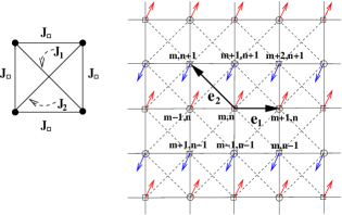
Figure 1: Couplings on an elementary plaquette of the 2D nn and nnn Ising model (left) and an example of the 4-fold degenerate SAF order (right). The SAF is also called columnar or stripe order in some recent literature. The degeneracy of the SAF state is due to the $Z_{2}\otimes Z_{2}$ symmetry with respect to the spins of each of the sublattices (labeled by circles or squares) being flipped. The lattice vectors are parameterized by the integers $(m,n)$ in the skewed basis $\mathbf{r}=m\mathbf{e}_{1}+n\mathbf{e}_{2}$.

The spin-pseudospin model (3) and some of its modifications were proposed and analyzed in the earlier related work GC04 ; GCStack04 ; CGEPL05 ; GCFNT05 in the context of the quarter-filled ladder compound $\rm NaV_{2}O_{5}$, where the pseudospins correspond to the charge degrees of freedom. For the physically interesting couplings GCFNT05 the classical Ising model ($\Omega=0$) orders into the 4-fold degenerate Super-Anti-Ferromagnetic (SAF) phase FanWu69 shown in Fig. 1. The SAF pattern appears in various contexts, and it is also called columnar or stripe order in some more recent literature. The SAF charge order occurs along with dimerization and gap in the spin sector GCFNT05 . That is what we called the spin-SAF transition GC04 ; GCStack04 ; CGEPL05 ; GCFNT05 . Note that the spin gap is due to the frozen phonon displacements at the spin-Peierls transition, while the charge plays the role of phonons at the spin-SAF transition.

The molecular-field approximation is applied for the pseudospins GC04 , while the spin sector is treated via minimization of the exact free energy of the dimerized Heisenberg $XXX$-chain

$$H_{\textrm{xxx}}=\sum_{n}J(1+(-1)^{n}\delta){\textbf{S}}_{n}{\textbf{S}}_{n+1}~{}.$$ (4)

The specific free energy of the spin chain $f_{s}(T,\delta)$ is an analytic function at $T\neq 0$ and can be expanded over $\delta$ as $f_{s}(T,\delta)=f_{s}(T,0)-\frac{J}{2}\eta(T,0)\delta^{2}+\mathcal{O}(\delta^{4})$, where $\eta(T,0)$ is called the static dimerization susceptibility.

$\bullet$ Spin-SAF phase transition. XY Spin Chain: Free Fermions. – It is straightforward to obtain in a closed form the specific free energy of the XY spin chain mapped onto the spinless non-interacting Jordan-Wigner fermions. To leading order GC04

$$\eta^{\textrm{\tiny XY}}(T,0)=\frac{1}{\pi}\ln\frac{\mathbb{C}J}{T}+\mathcal{O}\Big{(}\frac{T^{2}}{J^{2}}\Big{)}~{},$$ (5)

where $\mathbb{C}\equiv\frac{4}{\pi\textrm{e}^{1-\gamma}}$, $\gamma=0.5772...$ is Euler’s constant. In the region $\mathcal{J}<\mathcal{J}_{c}$ (where $\mathcal{J}_{c}=2\Omega$ is the mean-field value of the QCP of the IMTF (1) GCFNT05 ), the critical temperature is given by the BCS-type solution

$$T_{c}\approx\mathbb{C}J\textrm{exp}\Big{[}-\frac{\pi J}{\varepsilon^{2}}(\mathcal{J}_{c}-\mathcal{J})\Big{]}~{}.$$ (6)

The ground-state dimerization is

$$\delta\approx\frac{4}{\mathrm{e}}\textrm{exp}\Big{[}-\frac{\pi J}{\varepsilon^{2}}(\mathcal{J}_{c}-\mathcal{J})\Big{]},~{}~{}T=0~{}.$$ (7)

In the case of free fermions the spin gap depends linearly on dimerization, $\Delta^{\textrm{\tiny XY}}=J\delta$. So the ratio of the zero-temperature spin gap ($\Delta_{\circ}$) and the critical temperature (a.k.a the BCS ratio) in the regime $\mathcal{J}_{c}<\mathcal{J}$ is

$$\frac{\Delta_{\circ}^{\textrm{\tiny XY}}}{T_{c}}=\frac{4}{\mathrm{e}\mathbb{C}}=\frac{\pi}{\mathrm{e}^{\gamma}}=1.76...~{},$$ (8)

which coincides exactly with the classical result for the superconducting gap in the BCS theory AGD .

$\bullet$ Spin-SAF phase transition. XXX Spin Chain: Interacting Fermions – sine-Gordon Model. – The Heisenberg spin chain can be mapped onto the model of interacting Jordan-Wigner spinless fermions, and the low-energy sector of the fermionic Hamiltonian in its turn can be bosonized Tsvelik . Neglecting the marginal term, the dimerized spin chain maps onto the sine-Gordon model Tsvelik

$$v^{-1}H_{\mathrm{sG}}=\frac{1}{2}\int dx\big{(}\Pi^{2}+(\partial_{x}\phi)^{2}\big{)}+2\mu\int dx\cos\sqrt{2\pi}\phi~{},$$ (9)

where $v=\frac{\pi}{2}J$ is the bosonic velocity and $\mu=\frac{A_{\epsilon}}{\pi}\delta$. The relevant perturbation of the free bosonic part of the Hamiltonian (9) comes from the spin dimerization term $(-1)^{n}{\textbf{S}}_{n}{\textbf{S}}_{n+1}\sim A_{\epsilon}\cos\sqrt{2\pi}\phi$. The amplitude $A_{\epsilon}$ is not known exactly yet, but according to the approximate calculations of Orignac Orignac04

$$A_{\epsilon}=\frac{3}{\pi^{2}}\Big{(}\frac{\pi}{2}\Big{)}^{\frac{1}{4}}$$ (10)

Using the sine-Gordon model (9) to approximate the low-energy sector of the dimerized Heisenberg chain (4), the free energy of the latter reads to leading order Tsvelik ; OrignacChitra04

$$f_{s}(T,\delta)=-Jt_{\circ}-\frac{1}{3}\frac{T^{2}}{J}-\frac{1}{2}\frac{J^{2}a_{\circ}}{T}\delta^{2}~{},~{}~{}\textrm{where}~{}~{}a_{\circ}\equiv\frac{1}{4}\bigg{(}\frac{\Gamma(1/4)}{\Gamma(3/4)}\bigg{)}^{2}A_{\epsilon}^{2}\equiv\vartheta_{1}A_{\epsilon}^{2}~{},$$ (11)

and $t_{\circ}\equiv\ln 2-\frac{1}{4}=0.4431...$. Then the dimerization susceptibility to lowest order

$$\eta(T,0)=\frac{a_{\circ}J}{T}~{}.$$ (12)

This function was first calculated by Cross and Fisher CF79 for their spin-Peierls transition theory. The amplitude $A_{\epsilon}$ (10) suggested by Orignac Orignac04 gives $a_{\circ}=0.253418$, very close to the original bosonization result $a_{\circ}^{\textrm{\tiny CF}}\approx 0.26$ CF79 .

The interactions of the Jordan-Wigner spinless fermions of the XXX chain modify considerably the critical properties of the Ising-XXX model (3). The inverse dependence $\eta\propto T^{-1}$ (12) results in the power-law dependence of $T_{c}$ on couplings:

$$T_{c}=\vartheta_{1}A_{\epsilon}^{2}\frac{\varepsilon^{2}}{\mathcal{J}_{c}-\mathcal{J}}~{},~{}~{}\mathcal{J}<\mathcal{J}_{c}.$$ (13)

The phase diagram of the Ising-XXX model is shown in Fig. 2.

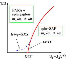
Figure 2: Phase diagram of the coupled Ising-XXX model. Axes are not in scale. The solid red line shows the critical temperature $T_{c}$ separating the disordered and SAF phases of the decoupled IMTF. Its QCP corresponds to $\mathcal{J}_{c}=2\Omega$ in the mean-field approximation. $(\mathcal{J}\equiv J_{1}+J_{2})$. The dashed blue line shows $T_{c}$ separating the disordered + spin gapless phase from the spin-SAF phase of the coupled Ising-XXX model.

From the ground-state specific energy of the sine-Gordon model Baxter ; AlZam95

$$f_{\mathrm{sG}}(0,\mu)=-v\frac{M^{2}}{4}\tan\frac{\pi}{6}~{},~{}\textrm{where}~{}~{}M=\frac{2}{\sqrt{\pi}}\bigg{(}\pi\mu\frac{\Gamma(3/4)}{\Gamma(1/4)}\bigg{)}^{2/3}\frac{\Gamma(1/6)}{\Gamma(2/3)}$$ (14)

($M$ is the dimensionless soliton mass) we get the ground-state energy of the Heisenberg chain (4):

$$f_{s}(0,\Delta_{\circ})=-Jt_{\circ}-\frac{1}{2\pi\sqrt{3}}\frac{\Delta_{\circ}^{2}}{J}~{},$$ (15)

where the zero-temperature spin gap $\Delta_{\circ}=\frac{\pi}{2}JM$ is related to the dimerization as follows:

$$\Delta_{\circ}=J\sqrt{\pi}\bigg{(}\frac{\Gamma(3/4)}{\Gamma(1/4)}\bigg{)}^{2/3}\frac{\Gamma(1/6)}{\Gamma(2/3)}A_{\epsilon}^{2/3}\delta^{2/3}~{}.$$ (16)

The ground-state spin gap:

$$\Delta_{\circ}=\vartheta_{2}A_{\epsilon}^{2}\frac{\varepsilon^{2}}{\mathcal{J}_{c}-\mathcal{J}}~{},~{}~{}\textrm{where}~{}~{}\vartheta_{2}\equiv\frac{2}{3}\sqrt{\frac{\pi}{3}}\bigg{(}\frac{\Gamma(3/4)}{\Gamma(1/4)}\bigg{)}^{2}\bigg{(}\frac{\Gamma(1/6)}{\Gamma(2/3)}\bigg{)}^{3}$$ (17)

Combining Eqs. (13,17) we obtain the BCS ratio:

$$\frac{\Delta_{\circ}}{T_{c}}=\frac{\vartheta_{2}}{\vartheta_{1}}=6\sqrt{3}\frac{\big{(}\Gamma(1/3)\big{)}^{9}}{\big{(}\Gamma(1/4)\big{)}^{8}}=2.47...$$ (18)

The same BCS ratio for the spin-Peierls transition was first obtained by Orignac and Chitra OrignacChitra04 . We would like to stress that the above result is exact for the IMTF coupled to the sine-Gordon model, i.e., when the marginal terms in the Heisenberg spin Hamiltonian are neglected. Similar to the non-interacting result (8), the ratio (18) does not depend on the microscopic parameters of the model, and even the dimerization amplitude $A_{\epsilon}$ cancels. In this sense we interpret this as a universal result. The interactions renormalize the BCS ratio away from the free fermionic value of 1.76.

$\bullet$ Conclusions. –The BCS ratio in the interacting Ising-XXX model is calculated. Similar to the classical free-fermionic case, this value is also universal in the sense that is does not depend on the microscopic parameters of the model. We conjecture that it must be the same for various types of the Peierls-like transitions where the spin gap is accompanied by the structural, orbital or charge order. An extension of these results taking into account marginal terms of the spin chain Hamiltonian is warranted.

$\bullet$ Acknowledgements. – I am very grateful to C. Gros, J. Leeson for the earlier spin-SAF theory collaborations, and to S.L. Lukyanov for numerous enlightening discussions. The author acknowledges financial support from NSERC (Canada) and the Laurentian University Research Fund.

References

- (1) See, e.g., J.-P. Pouget, Eur. Phys. J. B 20, 321 (2001); Erratum: ibid, 24, 415 (2001).
- (2) M.C. Cross and D.S. Fisher, Phys. Rev. B 19, 402 (1979).
- (3) K.I. Kugel and D.I. Khomskii, Usp. Fiz. Nauk 136, 621 (1982); [Sov. Phys. Usp. 25(4), 231 (1982)].
- (4) A. M. Oles, Acta Phys. Polon. A 118, 212 (2010).
- (5) D.I. Khomskii and T. Mizokawa, Phys. Rev. Lett. 94, 156402 (2005).
- (6) M.V. Mostovoy and D.I. Khomskii, Solid St. Comm. 113, 159 (1999); M.V. Mostovoy, D.I. Khomskii, and J. Knoester, Phys. Rev. B 65, 064412 (2002).
- (7) G.Y. Chitov and C. Gros, Phys. Rev. B 69, 104423 (2004).
- (8) G.Y. Chitov and C. Gros, J. Phys.: Condens. Matter 16, L415 (2004).
- (9) C. Gros and G.Y. Chitov, Europhys. Lett. 69, 447 (2005).
- (10) G.Y. Chitov and C. Gros, Low Temperature Physics 31, 722 (2005) [Fizika Nizkikh Temperatur 31, 952 (2005)].
- (11) B. Yan, M.M. Olmstead, and P.A. Maggard, J. Am. Chem. Soc. 129, 12646 (2007).
- (12) C. Fan and F.Y. Wu, Phys. Rev. 179, 560 (1969).
- (13) A.M. Tsvelik, Quantum Field Theory in Condensed Matter Physics, Second Edition, (Cambridge University Press, Cambridge, 2003).
- (14) See, e.g., A.A. Abrikosov, L.P. Gorkov, and I.E. Dzyaloshinski, 1963, Methods of Quantum Field Theory in Statistical Physics (Dover, New York).
- (15) Al.B. Zamolodchikov, Int. J. Mod Phys. A 10, 1125 (1995).
- (16) E. Orignac, Eur. Phys. J. B 39, 335 (2004).
- (17) E. Orignac and R. Chitra, Phys. Rev. B 70, 214436 (2004).
- (18) R.J. Baxter, Exactly Solved Models in Statistical Mechanics (Academic Press, London, 1982).