A new simple class of superpotentials in SUSY Quantum Mechanics

Abstract

In this work we introduce the class of quantum mechanics superpotentials $W(x)=g\varepsilon(x)x^{2n}$ and study in details the cases $n=0$ and $1$. The $n=0$ superpotential is shown to lead to the known problem of two supersymmetrically related Dirac delta potentials (well and barrier). The $n=1$ case result in the potentials $V_{\pm}(x)=g^{2}x^{4}\pm 2g|x|$. For $V_{-}$ we present the exact ground state solution and study the excited states by a variational technic. Starting from the ground state of $V_{-}$ and using logarithmic perturbation theory we study the ground states of $V_{+}$ and also of $V(x)=g^{2}x^{4}$ and compare the result got by this new way with other results for this last potential in the literature.

I Introduction

Supersymmetric quantum mechanics (SUSY QM) was first introduced by E. Witten Witten1 Witten2 , as a simplified model (a $0+1$ dimensional field theory) to study the possibility of SUSY breaking. Soon it became a research branch in itself, a way of getting new solutions to problems in quantum mechanics Cooper Bagchi Junker Elso . Of particular interest, to our work below, we must cite the many papers in the literature BenderLPT3 CooperLPT BenderLPT1 BenderLPT2 SukhatmeLPT LeeLPT Boya2 Guilarte devoted to the development of technics for treating the anharmonic oscillator $V(x)=\omega^{2}x^{2}+g^{2}x^{4}$, and other related potentials, which in general do not have exact solutions.

In this work we present a new simple class of superpotentials in SUSY QM, in the form $W(x)=g\varepsilon(x)x^{2n}$ with $n=0,1,2,\ldots$. The first example of this class, i.e., the case $n=0$, was studied long ago in Boya and revisited in Plyushchay1 and Plyushchay2 . One of our results is an analytic solution for the ground state wave function of the potential $V(x)=g^{2}x^{4}-2g|x|$, an amazing result, considering that analytic solutions do not exist for anharmonic oscillators. Another result is a new perturbative solution for the ground state of the potential $V(x)=gx^{4}$, starting from the solution for the potential $V(x)=g^{2}x^{4}-2g|x|$. Excited states of the potentials $V_{\pm}(x)=g^{2}x^{4}\pm 2g|x|$ are also studied by a variational approximation.

The paper is organized as folows. In Sec. II, we make a brief introduction to the well known case of superpotentials, which are monomials of odd powers of $x$, as well as to the SUSY breaking ones, which are monomials of even powers of $x$. More details of these solutions can be found in Cooper and FMarques . In Sec. III, we study solutions related to the class of simple superpotentials of the form $W(x)=g\varepsilon(x)x^{2n}$ ($n=0,1,2,\ldots$), where $\varepsilon(x)$ is the sign function. The simple analytical solution for the ground state of the corresponding SUSY system is shown, the already known case $n=0$ is revised and the case $n=1$ is studied in more details. The first one is the ilustrative example of the Dirac delta well and barrier potentials, which are shown to be SUSY partner potentials associated with the superpotential $W(x)=g\varepsilon(x)$. The second one, $W(x)=g\varepsilon(x)x^{2}$, allows us to find an analytical solution for the ground state of the potential $V(x)=g^{2}x^{4}-2g|x|$. In Sec. III.1 and Sec. III.2, we study the excited states of the potentials $V_{\pm}(x)=g^{2}x^{4}\pm 2g|x|$ which are derived from $W(x)=g\varepsilon(x)x^{2}$. After discussing that exact solutions for the excited states cannot be obtained, we apply a variational method (Sec. III.1) to find approximate solutions for the energy levels and the wave functions. In Sec. III.2, a new perturbative approach to the ground state of the potentials $V(x)=gx^{4}$ and $V(x)=g^{2}x^{4}+2g|x|$ is presented. Finally, a discussion of the results is presented in the Conclusions.

II Our Notation and Definitions on SUSY QM

Let us briefly summarize some main concepts in SUSY QM. For simplicity, we will work in a system of units with the Planck’s constant set as $\hbar=1$ and the particle mass set as $m=1/2$ (that is $2m=1$). We start by defining the operators $A^{\dagger}$ and $A$:

$$A^{\dagger}=W(x)-ip\qquad\text{and}\qquad A=W(x)+ip\;\text{,}$$ (1)

where $W(x)$ is a given function of $x$ and $p=-id/dx$ is the momentum operator. From these operators we can construct two hamiltonians:

$$H_{-}=A^{\dagger}A\qquad\text{and}\qquad H_{+}=AA^{\dagger}\;\text{,}$$ (2)

which in terms of $p$ and $W(x)$ result in: $H_{\pm}=p^{2}+V_{\pm}$. The potentials $V_{\pm}$ are given by the equations ($W^{\prime}\equiv dW/dx$):

$$V_{\pm}(x)=W(x)^{2}\pm W^{\prime}(x)\;\text{,}$$ (3)

which are Riccati’s equations.

These equations can be understood in two ways. One way is: given $W(x)$, we can define the hamiltonians $H_{\pm}$ with potentials $V_{\pm}(x)$. The other is: given the potential $V_{-}(x)$ (or $V_{+}(x)$), by solving one of the Riccati’s equations, $W(x)$ can be found, the operators $A$ and $A^{\dagger}$ constructed and the partner potential $V_{+}(x)$ (or $V_{-}(x)$) can be found.

The ground state of a SUSY system is defined as the zero energy state of $H_{-}$ (this is a choice; changing the function $W(x)\rightarrow-W(x)$ will change the roles of $H_{-}$ and $H_{+}$). As $H_{-}=A^{\dagger}A$, its ground state wave function $\psi_{0}^{-}(x)$ can be got by imposing that it is annihilated by the operator $A$, that is:

$$A\psi_{0}^{-}(x)=\left(W(x)+\frac{d}{dx}\right)\psi_{0}^{-}(x)=0\;\text{.}$$

The solution is given by:

$$\psi_{0}^{-}(x)=\mathcal{N}\exp{\left\{-\int^{x}W(y)dy\right\}}\;\text{.}$$ (4)

This is a good, physicaly meaningful solution, provided that the function (4) is normalizable. Otherwise, a zero energy solution does not exist and SUSY is said to be broken. As it is easy to see, superpotentials obeying the rule of being positive ($W(x)>0$) for $x>0$ and negative ($W(x)<0$) for $x<0$ shall manifest SUSY.

Then, starting from $W(x)$, we have two partner hamiltonians, $H_{-}$ and $H_{+}$, one of them ($H_{-}$, in our choice) having a ground state $\psi_{0}^{-}$ with energy $E_{0}^{-}=0$ and a tower of other states: bound states with energies $E_{n}^{-}>0$, $n=1,2,3,\ldots$ or scattering states with energies $E^{-}>0$. The hamiltonian $H_{+}$ has bound energy levels $E_{n-1}^{+}$, $n=1,2,3,\ldots$ with energies related to the energies of $H_{-}$ by the relation: $E_{n-1}^{+}=E_{n}^{-}$ or scattering energies $E^{+}>0$. Moreover, the eigenfunctions of $H_{-}$ and $H_{+}$ are related according to:

$$\psi_{n-1}^{+}=\left(E_{n}^{-}\right)^{-1/2}A\psi_{n}^{-}$$ (5)

$$\psi_{n}^{-}=\left(E_{n-1}^{+}\right)^{-1/2}A^{\dagger}\psi_{n-1}^{+}\;\text{.}$$ (6)

The simplest class of superpotentials manifesting supersymmetry are monomials of odd power in $x$ , that is:

$$W(x)=gx^{2n+1}\quad\text{,}\;n=0,1,2,\ldots\;\text{.}$$ (7)

Using the Riccati equation (3), we have for the partner potentials:

$$V_{\pm}(x)=W(x)^{2}\pm W^{\prime}(x)=g^{2}x^{4n+2}\pm g(2n+1)x^{2n}\;\text{.}$$ (8)

The ground (normalizable) state of $H_{-}=p^{2}+V_{-}$, with energy $E_{0}^{-}=0$ (see Eq. (4)) is given by:

$$\psi_{0}^{-}(x)=\mathcal{N}\exp{\left\{\frac{-gx^{2n+2}}{(2n+2)}\right\}}\;\text{.}$$ (9)

The first example of a superpotential of the class (7) is $W(x)=gx$. In this case, the associated partner potentials are:

$$V_{\pm}(x)=g^{2}x^{2}\pm g\;\text{,}$$ (10)

which are simply the potentials of two harmonic oscillators of the same frequency, with a constant energy shift $g$ added or subtracted. The ground state of $H_{-}$ have $E_{0}^{-}=0$. Its excited states and the states of $H_{+}$ are given by $E_{n}^{-}=E_{n-1}^{+}=2ng$, for $n=1,2,3,\ldots$.

We will not pursuit the study of this class of superpotentials because they are well known. We only mention that the next example of this class, $W(x)=gx^{3}$, corresponds to the potentials $V_{\pm}(x)=g^{2}x^{6}{\pm}3gx^{2}$ and their ground state solution is given by (9) with $n=1$.

On the other hand, the class of superpotentials that are monomials in even powers of $x$, does not give a normalizable zero energy solution to (4) and SUSY is broken. However, we can introduce the sign function $\varepsilon(x)$ and consider superpotentials of the form $W(x)=g\varepsilon(x)x^{2n}$. For this class of superpotentials, a normalizable ground state exists and SUSY is not broken. Thus, in the following we study this class of superpotentials, specially the $n=0$ and $n=1$ cases.

III The class of Superpotentials of the form $W(x)=g\varepsilon(x)x^{2n}$

The case $n=0$ must be treated separately. So, let us consider the superpotential:

$$W(x)=g\varepsilon(x)\;\text{,}$$ (11)

where $g$ is a positive constant. For this superpotential (11) the Riccati equations (3) give the following SUSY partner potentials:

$$V_{\pm}(x)=W(x)^{2}\pm W^{\prime}(x)=\pm 2g\delta(x)+g^{2}\;\text{,}$$ (12)

where $\delta(x)$ is the Dirac delta function. $V_{-}$ is a delta well, while $V_{+}$ is a delta barrier, with the energy of the ground state displaced by $g^{2}$. The corresponding Schrödinger equations are:

$$-\psi^{\pm\prime\prime}(x)\pm 2g\delta(x)\psi^{\pm}(x)=\left(E^{\pm}-g^{2}\right)\psi^{\pm}(x)\;\text{.}$$ (13)

Their solutions are well known Boya Plyushchay1 Plyushchay2 . The well ($V_{-}$) has a single bound state with energy level $E_{0}^{-}=0$, binding energy $g^{2}$, and wave function given by:

$$\psi_{0}^{-}(x)=\sqrt{g}e^{-g|x|}\;\text{.}$$ (14)

All the other eigenstates are plane waves in continuous spectra of energies, the lowest one starting with $E=g^{2}$. Simple scattering solutions of the well $V_{-}$ and the barrier $V_{+}$ can be written as:

$$\psi_{I}^{\pm}(x)=\mathcal{A}_{\pm}e^{ikx}+\mathcal{B}_{\pm}e^{-ikx}\quad,\qquad x\leq 0$$ (15)

$$\psi_{II}^{\pm}(x)=\mathcal{C}_{\pm}e^{ikx}+\mathcal{D}_{\pm}e^{-ikx}\quad,\qquad x\geq 0\;\text{,}$$ (16)

where $k=\sqrt{E^{\pm}-g^{2}}$ with $E^{\pm}>g^{2}$ and the respective constants are related according to the bondary conditions $\psi_{II}(0)=\psi_{I}(0)$ and $\psi^{\prime}_{II}(0)=\psi^{\prime}_{I}(0)\pm 2g\psi(0)$ required by the Dirac delta potential.

Summarizing: the hamiltonian $H_{-}$ has one ground state with energy $E_{0}^{-}=0$ and continuum of states with energies $E^{-}>g^{2}$ and $H_{+}$ has a continuum of states with $E^{+}>g^{2}$.

To see the role of the supersymmetry in this system, let us consider a particle crossing the well (or hitting the barrier), coming from $x=-\infty$, such that we can choose $\mathcal{D}_{\pm}=0$. With the apropriate boundary conditions through $x=0$, we can determine $\mathcal{B}_{\pm}$ and $\mathcal{C}_{\pm}$, getting the scattered and the transmited solutions as functions of the incident amplitudes $\mathcal{A}_{\pm}$. The results can be written as:

$$\qquad\psi_{I}^{\pm}(x)=\mathcal{A}_{\pm}\left\{e^{ikx}+i\frac{\frac{(\mp g)}{k}}{\left(1-i\frac{(\mp g)}{k}\right)}e^{-ikx}\right\} ,\qquad x\leq 0$$ (17)

$$\qquad\psi_{II}^{\pm}(x)=\mathcal{A}_{\pm}\frac{1}{\left(1-i\frac{(\mp g)}{k}\right)}e^{ikx} ,\qquad x\geq 0\;\text{.}$$ (18)

It is easy to verify that the solutions $\psi^{-}$ and $\psi^{+}$ are related by the supersymmetry equations (5) and (6). For example, by applying the operator $A$ to $\psi_{I}^{-}(x)$ we get:

$$A\psi_{I}^{-}(x) \propto\left(g\varepsilon(x)+\frac{d}{dx}\right)\left\{e^{ikx}+i\frac{\frac{g}{k}}{\left(1-i\frac{g}{k}\right)}e^{-ikx}\right\}$$

$$\propto\left\{e^{ikx}+i\frac{\frac{-g}{k}}{\left(1-i\frac{-g}{k}\right)}e^{-ikx}\right\}\propto\psi_{I}^{+}(x)\;\text{,}$$

explicitly showing the manifestation of the supersymmetry of the system.

Let us now consider the superpotential:

$$W(x)=g\varepsilon(x)x^{2}\;\text{,}$$ (19)

where here also, $g$ is a positive constant. The two partner potentials are given by:

$$V_{\pm}(x)=W(x)^{2}\pm W^{\prime}(x)=g^{2}x^{4}\pm 2g|x|\;\text{.}$$ (20)

In these potentials a term $\delta V=\pm 2gx^{2}\delta(x)$ has been dropped. The reason is that for the wave functions involved in this problem its action is null. As the potentials $V_{\pm}(x)\rightarrow\infty$ for $x\rightarrow\pm\infty$, the spectra of $H_{\pm}=p^{2}+V_{\pm}$ are discrete and their eigenfunctions are normalizable. If $\delta V$ is treated as a perturbative correction to $H_{\pm}$, its action would be non null only if $\int_{-\infty}^{\infty}dx\,x^{2}\delta(x)|\psi(x)|^{2}\neq 0$. But this condition requires a wave function that near $x=0$ behaves like $f(x)/x$ with $f(0)\neq 0$, which is non normalizable and is not in the spectra of $H_{\pm}$. On the other side, treated as part of $H_{\pm}$, the term $\delta V$ could give non trivial boundary conditions for $d\psi/dx$ at $x=0$. To study this possibility we must integrate the Schrödinger equation in the interval $x=(-\epsilon,\epsilon)$ for $\epsilon\rightarrow 0$. A non null effect of $\delta V$ only comes if $\int_{-\epsilon}^{\epsilon}dx\,x^{2}\delta(x)\psi(x)\neq 0$, which would require a $\psi(x)$ behaving like $f(x)/x^{2}$ with $f(0)\neq 0$ that is also, out of the spectra of $H_{\pm}$.

Figure 1: Partner potentials $V_{-}(x)$ and $V_{+}(x)$ associated with the superpotential $W(x)=g\varepsilon(x)x^{2}$.

A representation of these potentials is given in Fig. 1. As can be seen, $V_{+}$ is a single well potential and $V_{-}$ a double well potential symmetric in $x$. The corresponding Schrödinger equations read:

$$\left(-\frac{d^{2}}{dx^{2}}+g^{2}x^{4}\pm 2g|x|\right)\psi^{\pm}(x)=E^{\pm}\psi^{\pm}(x)\;\text{.}$$ (21)

The wave function for the ground state of the double well potential $V_{-}(x)=g^{2}x^{4}-2g|x|$, has energy $E_{0}^{-}=0$ and is easily obtained from the equation:

$$0=A\psi_{0}=\left(g\varepsilon(x)x^{2}+\frac{d}{dx}\right)\psi_{0}\;\text{.}$$

The result (already normalized) is given by:

$$\psi_{0}(x)=\left(\frac{3}{2}\right)^{1/3}\frac{g^{1/6}}{\Gamma\left(1/3\right)^{1/2}}e^{-g|x|^{3}/3}\;\text{.}$$ (22)

This is an interesting result. As it is well known, exact analytic solutions for the ground (or any excited) state of the potentials $V(x)=g^{2}x^{4}$ or $V(x)=\omega^{2}x^{2}+g^{2}x^{4}$ cannot be obtained. So this exact solution for the potential $V_{-}$ is somewhat surprising. Another characteristic of this solution, is that it represents a single lump centered at $x=0$ (which is a local maximum of $V_{-}$) and it is not in the form, as naively expected, of two lumps centered at the two symmetric minima, $x=\pm(1/2g)^{1/3}$, of $V_{-}$ notwithstanding the fact that, in one dimension, any attractive well supports at least a bound state. This happens because the "volume” of each well is not big enough to support a bound state (this can be seen in a WKB analysis of the potential, or even more simply, by the Heisenberg uncertaint principle. We should only observe that this well size $\Delta x(\Delta E)^{1/2}$ is independent of $g$).

Let us now look for the excited states solutions. Inspired by the analytic method to solve the one-dimensional simple harmonic oscillator and by the form of the solution (22), we try a solution of the form :

$$\psi(x)=F(x)e^{-\nicefrac{{g|x|^{3}}}{{3}}}\;\text{.}$$ (23)

Subtituting (23) in the Schrödinger equation (21), it becomes:

$$F^{\prime\prime}-2g\varepsilon(x)x^{2}F^{\prime}(x)+EF(x)=0\;\text{.}$$ (24)

For the simple harmonic oscillator, the same steps would lead us to the Hermite equation. In our case, we get the equation (24), which is, for a particular choice of parameters, the Triconfluent Heun equationRonv .

We can go on, look for solutions for the equation (24) through a power series method. Assuming that $F(x)$ can be written as:

$$F(x)=\sum_{j=0}^{\infty}a_{j}x^{j}$$ (25)

and substituting this expression for $F(x)$ in the differential equation (24), we find:

$$\sum_{j=0}^{\infty}j(j-1)a_{j}x^{j-2}-2g\varepsilon(x)\sum_{j=0}^{\infty}ja_{j}x^{j+1}+E\sum_{j=0}^{\infty}a_{j}x^{j}=0\;\text{.}$$

Renaming indices and rearranging terms, we have:

$$2a_{2}+Ea_{0}+\sum_{j=1}^{\infty}\left[(j+2)(j+1)a_{j+2}-2g\varepsilon(x)(j-1)a_{j-1}+Ea_{j}\right]=0\;\text{.}$$

Then, given $a_{0}$ e $a_{1}$, this equation is satisfied if the coefficients $a_{j}$, $j\geq 2$, are given by the three terms recursion relations:

$$a_{2}=-\frac{E}{2}a_{0} ,\qquad j=2\;\,\,$$ (26)

$$a_{j}=\frac{2g\varepsilon(x)(j-3)a_{j-3}-Ea_{j-2}}{j(j-1)} ,\qquad j\geq 3\;\text{.}$$ (27)

The corresponding recursion relation for the the harmonic oscilator potential, is a simple two terms recursion relation. To get a normalizable solution, we choose the values of $E$ so as to terminate the series in a polynomial. In this way we get the set of discretized values of the energy spectrum and the corresponding wave functions, that turn up to be the Hermite polynomials (see footnote).

In our case, the recurrence relation (27), is a three terms recurrence relation and there is no way of choosing a subset of values of $E$ to terminate the series in polynomials, so as to have a normalizable solution. Then, no analytic solution can be found and in the next sections we pass to look for approximate solutions. In Sec. III.1 a variational approximation is studied and in Sec. III.2 a perturbative approximation, that will allows us also, to study solutions for the potential $V(x)=gx^{4}$.

III.1 Looking for Approximate Solutions by a Variational Method

Let us first apply a variational method. The trial function that we are going to use is:

$$\phi(x)=\sum_{j=1}^{m}\alpha_{j}f_{j}(x)\;\text{,}$$ (28)

where $j=1,2,\ldots,m.$ and the coefficients $\alpha_{j}\in\mathbbm{C}$ are the variational parameters. The functions $f_{j}(x)$ are chosen to be:

$$f_{j}(x)=x^{j-1}e^{-\nicefrac{{g|x|^{3}}}{{3}}}\;\text{.}$$ (29)

This trial function corresponds to the previously used in the power series method, with the additional restriction of being a finite polynomial of degree $m-1$, instead of an infinite series in $x$.

For the harmonic oscillator, with a very similar choice of the trial function we would find exact solutions. In that case, the variational parameters would be, except for the normalization, the coefficients of the Hermite polynomials $\mathcal{H}_{n}(x^{2})$.

Before proceeding, let us consider a convenient change of variables. As can easily be seen, by making the rescaling: $x\rightarrow g^{-1/3}x$ it is possible to factor out of the hamiltonians $H_{\pm}$, the constant $g^{2/3}$, that is:

$$H_{\pm}=g^{2/3}\left(-\frac{d^{2}}{dx^{2}}+x^{4}\pm 2|x|\right)\;\text{.}$$ (30)

So, in the rest of this section, we will work with $g=1$ and after finding the energy eigenvalues, we can restore the dependence of the energy levels in $g$ by multiplying the results by a factor of $g^{2/3}$. The restoration of the corresponding wave functions (or trial functions), can also be obtained by rescaling $x\rightarrow g^{1/3}x$ in the results.

To go on with the variational method, we construct the expectation value of the energy with these trial functions:

$$E=\frac{\braket{\phi}{H_{\pm}}{\phi}}{\braket{\phi}{\phi}}=\frac{\sum\limits_{k=1}^{m}\sum\limits_{l=1}^{m}\alpha_{k}\alpha_{l}\braket{f_{k}}{H_{\pm}}{f_{l}}}{\sum\limits_{k=1}^{m}\sum\limits_{l=1}^{m}\alpha_{k}\alpha_{l}\braket{f_{k}}{f_{l}}}$$ (31)

and minimize $E$ with respect to the parameters $\alpha_{l}$. This condition gives the system of linear equations:

$$\sum_{l=1}^{m}((H_{\pm})_{kl}-ES_{kl})\alpha_{l}=0\;\text{,}$$ (32)

where we used the notation $H_{kl}=\braket{f_{k}}{H}{f_{l}}$ and $S_{kl}=\braket{f_{k}}{f_{l}}$. The values of $E$ that minimize the above system of equations are the eigenvalues of the matrix:

$$M_{kl}=\left(ES_{kl}-(H_{\pm})_{kl}\right)$$ (33)

and are obtained by solving the equation $\det{M}=0$. The wave functions corresponding to each of these eigenvalues are got by substituting the value of $E$ in the linear system above and solving for the parameters $\alpha_{k}$. The matrix elements that we need to construct $M_{kl}$ are:

$$S_{kl} =\braket{f_{k}}{f_{l}}=\int_{-\infty}^{+\infty}dx\,e^{-\frac{2}{3}|x|^{3}}x^{k+l-2}$$ (34)

$$\left(H_{\pm}\right)_{kl} =\braket{f_{k}}{H_{\pm}}{f_{l}}=\int_{-\infty}^{+\infty}dx\,e^{-\frac{2}{3}|x|^{3}}\left[-(l-1)(l-2)x^{k+l-4}+2(l\pm 1)\varepsilon(x)x^{k+l-1}\right]\;\text{.}$$ (35)

For $(k+l)$ odd, the integrands in (34) and (35) are odd functions and $S_{kl}=\left(H_{\pm}\right)_{kl}=0$. Otherwise, for $(k+l)$ even, we find:

$$S_{kl} =\left(\frac{3}{2}\right)^{\frac{k+l-4}{3}}\Gamma\left(\frac{k+l-1}{3}\right)$$ (36)

$$\left(H_{\pm}\right)_{kl} =-2\left(\frac{3}{2}\right)^{\frac{k+l-3}{3}}\left[\frac{(l-1)(l-2)-(l\pm 1)(k+l-3)}{(k+l-3)}\right]\Gamma\left(\frac{k+l}{3}\right)\;\text{.}$$ (37)

With these results, the matrix $M$ (33) gets the form:

$$M_{\pm}=\begin{pmatrix}(M_{\pm})_{11}&0&(M_{\pm})_{13}&0&&\ldots&&(M_{\pm})_{1m}\\ 0&(M_{\pm})_{22}&0&(M_{\pm})_{24}&&\ldots&&(M_{\pm})_{2m}\\ (M_{\pm})_{31}&0&(M_{\pm})_{33}&0&&\ldots&&(M_{\pm})_{3m}\\ \\ \vdots&\vdots&\vdots&\vdots&&\ddots&&\vdots\\ \\ (M_{\pm})_{m1}&(M_{\pm})_{m2}&(M_{\pm})_{m3}&(M_{\pm})_{m4}&&\ldots&&(M_{\pm})_{mm}\end{pmatrix}\;\text{.}$$ (38)

In this matrix, all elements in positions $(k,l)$, such that $(k+l)$ is odd are null, while those with $(k+l)$ even are given by (33) with $S_{kl}$ and $H_{kl}$ respectively given by (36) and (37). To find the energy values we must solve the equation: $\det{M}=0$.

Tables 1 and 2 show some results found for different number ($m$) of parameters and for $g=1$. For different values of $g$, the values in the Table must be multiplied by a factor of $g^{\nicefrac{{2}}{{3}}}$, as observed above.

Table 1: Energy values associated with $H_{-}$ calculated for different numbers of variational parameters.

$m$	$E^{-}_{0}$	$E^{-}_{1}$	$E^{-}_{2}$	$E^{-}_{3}$	$E^{-}_{4}$	$E^{-}_{5}$	$E^{-}_{6}$	$E^{-}_{7}$
1	0.00000
2	0.00000	2.04441
3	0.00000	2.04441	5.76541
4	0.00000	1.97852	5.76541	10.00191
5	0.00000	1.97852	5.54135	10.00191	14.94174
6	0.00000	1.97115	5.54135	9.49446	14.94174	20.37028
7	0.00000	1.97115	5.51302	9.49446	14.06558	20.37028	26.29953
8	0.00000	1.96991	5.51302	9.41370	14.06558	19.02962	26.29953	32.64399
9	0.00000	1.96991	5.50842	9.41370	13.90148	19.02962	24.43194	32.64399
10	0.00000	1.96963	5.50842	9.39868	13.90148	18.73498	24.43194	30.18755

Table 2: Energy values associated with $H_{+}$ calculated for different numbers of variational parameters.

$m$		$E_{0}^{+}$	$E_{1}^{+}$	$E_{2}^{+}$	$E_{3}^{+}$	$E_{4}^{+}$	$E_{5}^{+}$	$E_{6}^{+}$
1		2.31447
2		2.31447	6.13324
3		2.04493	6.13324	10.54940
4		2.04493	5.63655	10.54940	15.63469
5		1.99066	5.63655	9.66470	15.63469	21.21933
6		1.99066	5.53888	9.66470	14.30956	21.21933	27.28556
7		1.97666	5.53888	9.46567	14.30956	19.36916	27.28556	33.76558
8		1.97666	5.51611	9.46567	13.98107	19.36916	24.86727	33.76558
9		1.97235	5.51611	9.41524	13.98107	18.85787	24.86727	30.72924
10		1.97235	5.51007	9.41524	13.89369	18.85787	24.13659	30.72924

The results in Table 1 and 2 reflect the manifestation of SUSY in the system, at least with respect to the equality between the energy levels $E_{n}^{-}$ and $E_{n-1}^{+}$, $n>0$, of $H_{-}$ and $H_{+}$. As expected, the ground state energy of $H_{-}$ is zero and it is not equal to any energy of $H_{+}$. Moreover, for $n>0$, increasing the number of variational parameters, we find, mainly for the first levels, energies $E_{n}^{-}$ more and more closer to $E_{n-1}^{+}$.

Therefore, the better the trial we make, the closer we are to satisfy the equality between energy levels. Moreover, because the one parameter trial function for the ground state of $H_{-}$ has the same form of the exact (analytical) solution, the value $E_{0}^{-}=0$ found is exact and the condition of having a zero energy ground state is naturally satisfied.

Figure 2 shows the first energy levels of $H_{-}$ and $H_{+}$. We must remember that the values found are better for increasing number of variational parameters and for the lowest levels. Thus, for instance, we are supposed to find for the level $n=4$ a worse approximation than for the level $n=1$.

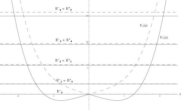
Figure 2: Scheme for the 5 first levels of $H_{-}$ (and 4 first levels of $H_{+}$) using 6 variational parameters.

The graphics in Fig. 3 show the approximations for the first levels eigenfunctions of $H_{-}$ and $H_{+}$, respectively. Those approximations were found using 6 variational parameters.

 

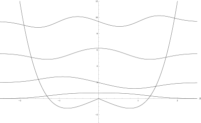
(a) Eigenfunctions of $H_{-}$

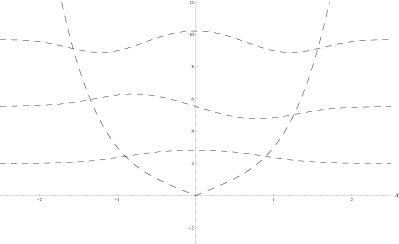
(b) Eigenfunctions of $H_{+}$

Figure 3: Eigenfunctions of the first levels of $H_{-}$ and $H_{+}$ for 6 variational parameters.

As expected, we see that the eigenfunctions found have well defined parity, interchanging even and odd solutions with even solutions for the ground states.

III.2 Looking for Approximate Solutions by a Logarithmic Perturbation Theory

We now apply a variant of the logarithmic perturbation theory (LPT) to our problem. LPT is explained with more details, for example, in Cooper , BenderLPT3 , CooperLPT , BenderLPT1 or SukhatmeLPT .

Starting from the known solution $\psi_{0}^{-}$ of $V_{-}$ we can perturbatively obtain the ground state of $V_{+}$, or for example, of the anharmonic potential $V(x)=x^{4}$. We start by writting:

$$V(x;\delta)=V_{0}(x)+\delta V_{1}(x)\;\text{,}$$ (39)

where:

$$V_{0}(x)=V_{-}(x)=x^{4}-2|x|$$ (40)

$$V_{1}(x)=4|x|\;\text{.}$$ (41)

Observe that $V(x;\delta=1)=V_{+}$ and that $V(x;\delta=1/2)=x^{4}$. As we only know the ground state of $V_{-}$ we can not go beyond the first order in the Rayleigh-Schrödinger perturbation theory. To bypass this difficult we will use the so called logarithmic perturbation theory where only the knowledge $\psi_{0}^{-}$ is required to calculate the ground state energy level of $V(x;\delta)$ to any order in $\delta$ (at least numerically). For that aim we consider the perturbed Schrödinger equation:

$$-\Psi"+(V_{0}+\delta V_{1})\Psi=E\Psi$$ (42)

and write the expansions:

$$E=E_{0}+\delta E_{1}+\delta^{2}E_{2}+\ldots$$ (43)

$$\Psi=\exp{(S_{0}+\delta S_{1}+\delta^{2}S_{2}+\ldots)}\;\text{,}$$ (44)

where $S_{1}$, $S_{2}$, etc. are functions and $E_{1}$, $E_{2}$, etc. are numbers to be determined. By substituting these expressions in the Schrödinger equation above and equating the terms of same powers in $\delta$ we get the set of equations:

$$S_{0}^{\prime\prime}+S_{0}^{\prime\,2} =-E_{0}+V_{2}$$ (45)

$$S_{1}^{\prime\prime}+2S_{0}^{\prime}S_{1}^{\prime} =-E_{1}+V_{1}$$ (46)

$$S_{2}^{\prime\prime}+2S_{0}^{\prime}S_{2}^{\prime}+S_{1}^{\prime\,2} =-E_{2}$$ (47)

$$S_{3}^{\prime\prime}+2S_{0}^{\prime}S_{3}^{\prime}+2S_{1}^{\prime}S_{2}^{\prime} =-E_{3}$$ (48)

$$\,\,\,\vdots$$

Starting with $E_{0}=0$ and $S_{0}=-|x|^{3}/3$, (that is, $\Psi_{0}(x)=\psi^{-}_{0}=\mathcal{N}e^{-\nicefrac{{|x|^{3}}}{{3}}}$), these equations can be recursively solved to get $E_{k}$ and $S_{k}$ to the desired order in $\delta$.

Eq. (46) can be rewritten as:

$$(S^{\prime}_{1}\exp{(2S_{0})})^{\prime}=(V_{1}-E_{1})\exp{(2S_{0})}\;\text{.}$$ (49)

By substituting $S_{0}=-|x|^{3}/3$ and $V_{1}=4|x|$ in this equation, integrating both sides in the interval $x=(-\infty,+\infty)$ and observing that the integrand of the left side goes exponentially to zero at both ends of the integration range, we get for $E_{1}$ the result:

$$E_{1} =\frac{\braket{\psi_{0}}{V_{1}(x)}{\psi_{0}}}{\braket{\psi_{0}}{\psi_{0}}}=\frac{\int_{-\infty}^{+\infty}dxe^{-\frac{2}{3}|x|^{3}}4|x|}{\int_{-\infty}^{+\infty}dxe^{-\frac{2}{3}|x|^{3}}}$$ (50)

$$=4\left(\frac{3}{2}\right)^{\nicefrac{{1}}{{3}}}\frac{\Gamma(2/3)}{\Gamma(1/3)}=2.31447\;\text{.}$$

Inserting this result for $E_{1}$ back into the same equation and integrating now in the interval $y=(0,x)$ we get:

$$S^{\prime}_{1}(x) =|\psi_{0}(x)|^{-2}\int_{0}^{x}dy|\psi_{0}(y)|^{2}\left[E_{1}-V_{1}(y)\right]$$ (51)

$$=e^{\frac{2}{3}|x|^{3}}\int_{0}^{x}dye^{-\frac{2}{3}|y|^{3}}\left[4\left(\frac{3}{2}\right)^{\nicefrac{{1}}{{3}}}\frac{\Gamma(2/3)}{\Gamma(1/3)}-4|y|\right]$$

$$=-2\left(\frac{2}{3}\right)^{1/3}e^{\frac{2}{3}|x|^{3}}\left[\frac{\Gamma(2/3)}{\Gamma(1/3)}\Gamma(1/3,2x^{3}/3)-\Gamma(2/3,2x^{3}/3)\right]\;\text{,}$$

where $\Gamma(\alpha,x)\equiv\int_{x}^{\infty}dt\,e^{-t}t^{\alpha-1}$ are the upper incomplete gamma functionsGrad .

The second order equation (47) can also be written in the form:

$$(S^{\prime}_{2}\exp{(2S_{0})})^{\prime}=(-S_{1}^{\prime\,2}-E_{2})\exp{(2S_{0})}\;\text{.}$$ (52)

Integrating this equation in the interval $x=(-\infty,+\infty)$, and observing that the integrand of the left side goes to zero at both ends of the integration range, we get $E_{2}$ as an integral over $S^{\prime}_{1}$:

$$E_{2}=-\frac{\braket{\psi_{0}}{S^{\prime}_{1}(x)^{2}}{\psi_{0}}}{\braket{\psi_{0}}{\psi_{0}}}=-\frac{3}{\Gamma(1/3)}\left(\frac{2}{3}\right)^{\nicefrac{{1}}{{3}}}\int_{0}^{\infty}dxe^{-\frac{2}{3}|x|^{3}}S^{\prime}_{1}(x)^{2}\;\text{.}$$ (53)

Substituting (51) in (53), we find:

$$E_{2}=-\frac{4}{\Gamma(1/3)}\left(\frac{2}{3}\right)^{\nicefrac{{2}}{{3}}}\left\{\frac{\Gamma(2/3)^{2}}{\Gamma(1/3)^{2}}I_{\nicefrac{{2}}{{3}}}\left(\tfrac{1}{3},\tfrac{1}{3}\right)+I_{\nicefrac{{2}}{{3}}}\left(\tfrac{2}{3},\tfrac{2}{3}\right)-2\frac{\Gamma(2/3)}{\Gamma(1/3)}I_{\nicefrac{{2}}{{3}}}\left(\tfrac{1}{3},\tfrac{2}{3}\right)\right\}\;\text{,}$$ (54)

where:

$$I_{\alpha}(x,y)=\int_{0}^{\infty}dt\,e^{t}t^{-\alpha}\Gamma(x,t)\Gamma(y,t)\;,\quad x>0\;,\quad y>0\;,\quad 0<\alpha<1\;\text{.}$$ (55)

Evaluating the integrals, the expression (54) gives $E_{2}=-0.43817$.

Sumarizing: up to the second order, the ground state energy of $V(x;\delta)$ is given by:

$$E(\delta)=E_{0}+\delta E_{1}+\delta^{2}E_{2}\;\text{,}$$ (56)

with $E_{0}=0$, $E_{1}=2.31447$ and $E_{2}=-0.43817$.

For $\delta=1$, we get for the ground state energy of $V_{+}$, the result: $E_{0}^{+}=1.87630$.

For $\delta=1/2$, we find the result $E_{0}^{x^{4}}=1.04769$ for the ground state energy of the the quartic anharmonic potential $V(x)=x^{4}$. This result can be compared with the exact one given in Cooper , noting that our “coupling” constant $g$ is related to their constant $\tilde{g}$ by: $g^{2/3}=\left(\frac{1}{4}\right)^{1/3}\tilde{g}^{1/3}$. Thus, multiplying our result by $\left(\frac{1}{4}\right)^{1/3}$, we find: $\tilde{E}_{0}^{x^{4}}=0.66000$, differing of Cooper only by about $1.2\%$.

On the other hand, comparing the value of $E_{0}^{+}$ found here with the most acurate result of the variational method (see Table 2), we see that they differ by about $4.9\%$, what does not seem very good. But, following the suggestion of CooperLPT or BenderBook , and substituting the expression (56) by the corresponding $[1,1]$ Padé approximant in $\delta$, we find:

$$E(\delta)=\frac{E_{0}E_{1}+(E_{1}^{2}-E_{0}E_{2})\delta}{E_{1}-E_{2}\delta}\;\text{,}$$ (57)

which results (for $\delta=1$) in $E_{0}^{+}=1.94605$. This result now differs from the result of Table 2 only by $1.3\%$. Doing the same for $\delta=1/2$ (and then multiplying by $\left(\frac{1}{4}\right)^{1/3}$), we find $\tilde{E}_{0}^{x^{4}}=0.66597$, differing from the result of Cooper et all Cooper by only $0.03\%$. A pretty good result.

IV Conclusions

In this paper we studied the class of superpotentials $W(x)=\varepsilon(x)x^{2n}$ in SUSY QM. After revisiting the case $n=0$ we went on studying in details the case $W(x)=\varepsilon(x)x^{2}$. As a result we got the exact solution for the ground state of the potential $V_{-}(x)=x^{4}-2|x|$, showed that exact solutions do not exist for the excited states and studied these states by a variational method. Finally, starting from the known ground state of $V(x)=x^{4}-2|x|$, we obtained the ground states for the potentials $V(x)=x^{4}$ and $V(x)=x^{4}+2|x|$, by using logarithmic perturbation theory. Comparision with other known results in the literature and in the paper are given.

Some other approaches and improvements can be used to study this class of superpotentials. In a forthcoming paper we analyze the solutions for the ground states of $V_{\pm}(x)=x^{4}\pm 2|x|$ by starting with the solutions of $V_{\pm}=x^{2}\pm C$ and using LPT and the $\delta$ expansion of Bender BenderLPT3 and Cooper CooperLPT .

Updated: .

References

• (1) E. Witten, Nucl. Phys. B 185 (1981) 513.
• (2) E. Witten, Nucl. Phys. B 202 (1982) 253.
• (3) F. Cooper, A. Khare, and U. Sukhatme, Supersymmetry in Quantum Mechanics. World Scientific, 2001.
• (4) B. K. Bagchi, Supersymmetry in Quantum and Classical Mechanics. Chapman & Hall/CRC, 2001.
• (5) G. Junker, Supersymmetric Methods in Quantum and Statistical Physics. Springer, Berlim, 1996.
• (6) E. Drigo Filho, Supersimetria aplicada à Mecânica Quântica. Editora Unesp, 2009.
• (7) C. M. Bender, Nuc. Phys. B (Proc. Suppl.) 11 (1989) 316-324.
• (8) F. Cooper, and P. Roy, Phys. Lett. A 143 (1990) 202-206.
• (9) C. M. Bender, K. A. Milton, M. Moshe, S. S. Pinsky, and L. M. Simmons Jr., Phys. Rev. Lett., 58 (1987) 2615.
• (10) C. M. Bender, K. A. Milton, M. Moshe, S. S. Pinsky, and L. M. Simmons Jr., Phys. Rev., D37 (1988) 1472.
• (11) T. Imbo, and U. Sukhatme, Am. Jour. Phys. 52 (1984) 140-146
• (12) C. Lee, Phys. Lett., A 267 (2000) 101-108.
• (13) L. J. Boya, M. Kmiecik, and A. Bohm, Phys. Rev. D35 (1987) 1255.
• (14) M. A. González León, J. Mateos Guilarte, and M. de le Torre Mayado, hep-th:0603225v1 29 Mar 2006.
• (15) L. J. Boya,Eur. J. Phys. 9 (1988) 139-144.
• (16) F. Correa, L. M. Nieto, and M. S. Plyushchay, Phys.Lett. B 659 (2008) 746-753.
• (17) V. Jakubský, L. M. Nieto, and M. S. Plyushchay, Phys.Lett. B 692 (2010) 51-56.
• (18) F. Marques, A study about the Supersymmetry in the context of Quantum Mechanics, University of Sao Paulo, Brazil (2011).
• (19) A. Ronveaux, Heun’s Differential Equations. Oxford University Press, 1995.
• (20) I. S. Gradshteyn, I. M. Ryzhik, Table of Integrals, Series and Products: Corrected and Enlarged Edition. Academic Press, Inc. San Diego, 1980.
• (21) C. M. Bender, and S. A. Orszag, Advanced Mathematical Methods for Scientists and Engineers. McGraw-Hill, 1978.