Beyond pure state entanglement for atomic ensembles

Abstract

We analyze multipartite entanglement between atomic ensembles within quantum matter-light interfaces. In our proposal, a polarized light beam crosses sequentially several polarized atomic ensembles impinging on each of them at a given angle $\alpha_{i}$. These angles are crucial parameters for shaping the entanglement since they are directly connected to the appropriate combinations of the collective atomic spins that are squeezed. We exploit such scheme to go beyond the pure state paradigm proposing realistic experimental settings to address multipartite mixed state entanglement in continuous variables.

Keywords: atomic ensembles, quantum interfaces, continuous variables, multipartite entanglement

1 Introduction

Experiments exploiting the quantum character of atom-light interactions are often carried out in the regime of cavity QED where, due to cavity, the coupling between individual atoms and photons, represented by the optical depth is highly enhanced. An alternative approach to achieve an efficient atom-photon coupling are atomic ensembles, where large optical depths are obtained due to to the macroscopic or mesoscopic number of atoms of the sample, as proposed initially by Kuzmich and coworkers [1].

Atomic ensembles typically refer to samples composed of $10^{6}$ to $10^{12}$ atoms. In the atomic ensembles the spin of each atom, $\hat{\bf{j}}_{i}$, originating either from its hyperfine structure or from its nuclear spin (e.g. alkaline-earth fermions) can be disregarded and the sample can be characterized by its collective spin $\hat{\bf{J}}=(\hat{J}_{x},\hat{J}_{y},\hat{J}_{z})=\sum_{i}\hat{\bf{j}}_{i}$. If the sample is polarized, the component of $\hat{\bf{J}}$ along the polarization axis can be approximated to a c-number, let’s say $\hat{J}_{x}=\sum_{i}\hat{j}_{x}^{i}\simeq\langle\hat{J}_{x}\rangle$, while the orthogonal components behave as conjugate canonical variables$[\hat{J}_{y},\hat{J}_{z}]=i\hbar\langle\hat{J}_{x}\rangle$. Such an elegant and simple description of polarized atomic ensembles makes them extremely appealing for quantum information processing in the domain of continuous variables.

The interaction between a polarized atomic ensemble and an off-resonant linearly polarized laser beam results – at the classical level – in a Faraday rotation. The latter refers to the rotation experienced by the polarization of light when it propagates through a magnetic medium, in our case the polarized atomic ensemble. Furthermore, this interaction leads to a quantum interface, i.e., an exchange of quantum fluctuations between the matter and the light. Seminal results exploiting such interface are the generation of atomic spin squeezed states produced by the interaction of coherent atomic sample and a squeezed light beam [1, 2], the realization of the atomic quantum memory [3] and the establishing of entangled state of two spatially separated atomic ensembles [4]. The above situations require a final projective measurement on the light (homodyne detection) that projects the atomic ensembles into their desired final state. This ”measurement induced” mapping of fluctuations between different physical systems provides a powerful tool to design quantum correlations. The potential applications of such a genuine quantum tool have just started. Among them are the application in quantum metrology [5, 6], quantum magnetometry [7] and quantum spectroscopy for detection of magnetic ordering in spinor Bose-Einstein condensates [8], or strongly correlated spin systems realized with ultracold atomic gases [9, 10, 11, 12].

A milestone achievement using quantum matter-light interfaces was the generation of entanglement between two spatially separated atomic ensembles [4] mediated by a single light beam propagating sequentially through both of them. In such setup, the entanglement between the atomic ensembles was established as soon as the light was measured, independently of the outcome of the measurement. However the detection of the entanglement thus generated, based on variance inequalities criteria [13, 14], is rather challenging. As shown in [4] its verification can be made feasible with the help of external magnetic fields applied to the ensembles. Nonetheless, it has been shown in [15] that entanglement verification without external magnetic fields is also possible if the light crosses through each sample at a given angle $\alpha_{i}$. In this setup, that we name ”geometrical”, the incident angles play a critical role since they can be used to shape both quantitatively and qualitatively, the entanglement between the atomic ensembles.

The geometrical scheme of entangling different atomic systems using quantum interfaces can be extended beyond the bipartite pure state setting to include both several parties and noise. Multipartite mixed states entanglement, has been mainly addressed for finite dimensional Hilbert spaces and it is poorly understood in all but the simplest situations. For instance, recent results suggesting the potential supremacy of noisy quantum computation versus pure state multipartite quantum computation[16, 17, 18] are highly intriguing. For continuous variables even less is known. Atomic-ensemble systems belong to the important class of continuous-variable states known as Gaussian, whose characterization and mathematical description is much simpler. For instance, the complete classification of three-mode Gaussian systems has been provided in [19, 20]. However, even in the simplest multipartite Gaussian scenario, the verification of the entanglement using variance inequalities [14] becomes a very intricate task in the atomic-ensemble setup. Here we address the generation and detection of multipartite entanglement in Gaussian mixed states in experimentally feasible systems using the geometrical scheme. In particular, we provide physical bounds on atomic ensembles’ parameters that lead to generation of bound entanglement, providing a guideline on their experimental accessibility. Bound entanglement refers to the entanglement which cannot be distilled, i.e., no pure state entanglement can be obtained from it by means of local operations and classical communication (LOCC). In the multipartite setting, a state can be bound entangled with respect to certain parties while distillable with respect to others. Although bound entanglement may seem useless for quantum information processing, it has been shown that for discrete systems it can be used for certain tasks (e.g. channel discrimination) or activated [21, 22, 23, 24, 25, 26].

A particular example of bound entanglement we are going to deal with is the so-called Smolin state [27]. In the discrete case, this state corresponds to a four qubit mixed state formed by an equal-weight mixture of Bell states that has the property that its entanglement can be unlocked. Moreover, it has been shown that it violates maximally a Bell inequality, being at the same time useless for secrete key distribution [23]. The Smolin state has been very recently addressed mathematically within the continuous variables stabilizer formalism[28]. Here we will perform its covariance matrix analysis that gives more insight into the nature of the state and demonstrate how such type of states can be experimentally realized using quantum light interfaces with atomic-ensembles.

Since both the atomic ensembles and the light assume a unified continuous-variable description and given the inherent Gaussian character of the setting we are considering, we use a covariance matrix formalism [29] to describe in a compact way the generation and manipulation of entanglement. Such a formalism, as we shall see, enlightens the possibilities offered by atomic samples as a quantum toolbox to generate many different types of continuous variables entangled states in an experimentally accessible way.

The paper is organized as follows. In Section 2 we review, for completeness, the description of matter and light as continuous variables systems, and describe the matter-light interaction in terms of an effective Hamiltonian and the corresponding evolution equations. Then we derive explicitly all the steps of the matter-light interface in terms of covariance matrices, symplectic transformations and Gaussian operations. In Section 3 we analyze the properties of the interface leading to mixed state entanglement with atomic ensembles. First, we consider the bipartite case in Section 3.1, setting the bounds on system parameters that produce mixed state entanglement. In Section 3.2 we move to multipartite bound entanglement in continuous variables. Here, we consider a general frame in which initially the atomic samples are in a thermal state with different amounts of noise. This allows us to set physical bounds on the generation of such type of entanglement in the CV scenario. In Section 3.3 we analyze the much more involved Smolin state[28]. We show that the geometrical setup we propose provides all the tools needed to generate and unlock the Smolin state, including a (quantum) random number generator. Finally, in Section 4 we present our conclusions.

2 Continuous Variables systems

2.1 The Faraday Interaction

The setting we are considering consists of several atomic ensembles and light beams, the latter playing the role of information carriers between the atomic samples. At a time, only a single light beam interacts with the atomic ensembles. In previous proposals, the light beam after interacting with the atomic ensembles was measured, inducing entanglement between the different samples (see e.g.[29, 30, 4, 15]). Here, we will have a closer look at the situation in which the light beam is not measured after the interaction. Such action, as we will see, acts as a truly quantum Gaussian random number generator. We will show that through such procedure one can generate multipartite mixed states, in particular bound entangled states.

As pointed out in the introduction, each atomic ensemble is described by its collective angular momentum $\mathbf{\hat{J}}=(\hat{J}_{x},\hat{J}_{y},\hat{J}_{z})$. Atoms are assumed to be all polarized along the $x$ direction (e.g. prepared in a particular hyperfine state) so that fluctuations in the $\hat{J}_{x}$ component of the collective spin are very low and this variable can be treated as a classical number $\hat{J}_{x}\approx\big{\langle}\hat{J}_{x}\big{\rangle}\equiv\hbar J_{x}=\hbar N_{\mathrm{at}}j$. By appropriate normalization the orthogonal spin components are made to fulfill the canonical commutation relation, $\left[\hat{J}_{y}/\sqrt{\hbar J_{x}},\hat{J}_{z}/\sqrt{\hbar J_{x}}\right]=i\hbar$. Notice that they have non-zero fluctuations. To stress the continuous variable character of the system, we rename the above variables as “position” and “momentum” :

$$\hat{x}_{A}=\frac{\hat{J}_{y}}{\sqrt{\hbar J_{x}}},\mbox{\hskip 56.9055pt}\hat{p}_{A}=\frac{\hat{J}_{z}}{\sqrt{\hbar J_{x}}}.$$ (1)

From now on we will use only the canonical variables $\hat{x}_{A},\hat{p}_{A}$ to refer to the atomic sample, where the subindex $A$ stands for atomic ensemble. Later on when dealing with different atomic ensembles the notation $\hat{x}_{A,n},\hat{p}_{A,n}$, when we refer to the $n$th atomic sample, will be used.

Light is taken to be out of resonance from any relevant atomic transition and linearly polarized along the $x$-direction. We use the Stokes description $\mathbf{\hat{s}}=(\hat{s}_{x},\hat{s}_{y},\hat{s}_{z})$ for the light polarization. The components $\hat{s}_{k}$ $(k=x,y,z)$ correspond to the differences between the number of photons (per unit time) with $x$ and $y$ linear polarizations, $\pm\pi/4$ linear polarizations and the two circular polarizations, i.e.,

$$\begin{array}[]{l}\displaystyle\hat{s}_{x}=\frac{\hbar}{2}(\hat{n}_{x}-\hat{n}_{y})=\frac{\hbar}{2}(\hat{a}_{x}^{\dagger}\hat{a}_{x}-\hat{a}_{y}^{\dagger}\hat{a}_{y}),\\[8.61108pt] \displaystyle\hat{s}_{y}=\frac{\hbar}{2}(\hat{n}_{\nearrow}-\hat{n}_{\searrow})=\frac{\hbar}{2}(\hat{a}_{x}^{\dagger}\hat{a}_{y}+\hat{a}_{y}^{\dagger}\hat{a}_{x}),\\[8.61108pt] \displaystyle\hat{s}_{z}=\frac{\hbar}{2}(\hat{n}_{\circlearrowleft}-\hat{n}_{\circlearrowright})=\frac{\hbar}{2i}(\hat{a}_{x}^{\dagger}\hat{a}_{y}-\hat{a}_{y}^{\dagger}\hat{a}_{x}).\end{array}$$ (2)

The Stockes operators are well suited for the microscopic description of interaction with atoms, however, effectively only the following macroscopic observables will be relevant: $\hat{S}_{k}=\int_{0}^{T}\hat{s}_{k}(t)\mathrm{d}t$, where $T$ is the duration of the light pulse. The so defined operators obey standard angular momentum commutation rules. The assumption of linear polarization along direction $x$ allows for the approximation $\hat{S}_{x}\approx\big{\langle}\hat{S}_{x}\big{\rangle}\equiv N_{ph}\hbar/2$. Once more, the remaining orthogonal components $\hat{S}_{y}$ and $\hat{S}_{z}$ are appropriately rescaled in order to make them fulfill the canonical commutation rule, $\left[\hat{S}_{y}/\sqrt{\hbar S_{x}},\hat{S}_{z}/\sqrt{\hbar S_{x}}\right]=i\hbar$. Straightforwardly, an equivalent equation to equation (1) arises:

$$\hat{x}_{L}=\frac{\hat{S}_{y}}{\sqrt{\hbar S_{x}}},\mbox{\hskip 56.9055pt}\hat{p}_{L}=\frac{\hat{S}_{z}}{\sqrt{\hbar S_{x}}},$$ (3)

which allows to treat the light polarization degrees of freedom on the same footing as the atomic variables.

In the situation in which a light beam propagates in the $YZ$ plain and passes through a single ensemble at angle $\alpha$ with respect to direction $z$, the atom-light interaction can be approximated to the following QND effective Hamiltonian (see [31] and references therein for a detailed derivation):

$$\hat{H}_{\mathrm{int}}^{\mathrm{eff}}(\alpha)=-\kappa\hat{p}_{L}(\hat{p}_{A}\cos{\alpha}+\hat{x}_{A}\sin{\alpha}).$$ (4)

The parameter $\kappa$ is the coupling constant with the dimension of the inverse of an action. Notice that such Hamiltonian leads to a bilinear coupling between the Stokes operator and the collective atomic spin operators. Evolution can be calculated through the Heisenberg equation for the atoms and using Maxwell-Bloch equation for light, neglecting retardation effects. The variables characterizing both systems (atom and light) transform according to the following equations ([31] and references therein):

$$\hat{x}_{A}^{\mathrm{out}} = \hat{x}_{A}^{\mathrm{in}}-\kappa\hat{p}_{L}^{\mathrm{in}}\cos\alpha,$$ (5a)

$$\hat{p}_{A}^{\mathrm{out}} = \hat{p}_{A}^{\mathrm{in}}+\kappa\hat{p}_{L}^{\mathrm{in}}\sin\alpha,$$ (5b)

$$\hat{x}_{L}^{\mathrm{out}} = \hat{x}_{L}^{\mathrm{in}}-\kappa(\hat{p}_{A}^{\mathrm{in}}\cos{\alpha}+\hat{x}_{A}^{\mathrm{in}}\sin{\alpha}),$$ (5c)

$$\hat{p}_{L}^{\mathrm{out}} = \hat{p}_{L}^{\mathrm{in}}.$$ (5d)

where the subscript in/out refers to the variable before/after the interaction. The above equations can be generalized to the case in which a single light beam $(\hat{x}_{L},\hat{p}_{L})$ propagates through many samples shining at the $n$th sample at a certain angle $\alpha_{n}$. A complete description taking into account inhomogeneities of the atomic samples or the light beams has been considered in [32].

Due to the strong polarization constraint, both the atomic ensembles and the light are initially Gaussian modes. Moreover, the Hamiltonian is linear in both atomic and light quadratures, and therefore quadratic in creation and annihilation operators. Such interaction Hamiltonians correspond to Gaussian transformations preserving the Gaussianity of the input state. These facts enable us to tackle the quantum atom-light interface within a covariance matrix formalism.

2.2 The atom light interface in the covariance matrix formalism

We start by reviewing the most basic concepts needed to describe Gaussian continuous-variable systems. For further reading, the reader is referred to [33, 34, 35] and references therein. For a general quantum system of $N$ pairs of canonical degrees of freedom (“position” and “momentum”), the commutation relations fulfilled by the canonical coordinates $\hat{R}=(\hat{x}_{1},\hat{p}_{1},\ldots,\hat{x}_{N},\hat{p}_{N})$ can be represented in a matrix form by the symplectic matrix $\mathcal{J}_{N}:[\hat{R}_{i},\hat{R}_{j}]=i\hbar(\mathcal{J}_{N})_{ij}$, $i,j=1,\ldots,2N$, where

$$\mathcal{J}_{N}=\bigoplus_{\mu=1}^{N}\mathcal{J},\quad\mathcal{J}=\left(\begin{array}[]{cc}0&1\\ -1&0\\ \end{array}\right).$$ (5f)

Gaussian states are, by definition, fully described by the first and second moments of the canonical coordinates. Hence, rather than describing them by their infinite-dimensional density matrix $\varrho$, one can use the Wigner function representation

$$W(\zeta)=\frac{1}{\pi^{N}\sqrt{\det\gamma}}\exp\left[-(\zeta-d)^{T}\gamma^{-1}(\zeta-d)\right],$$ (5g)

which is a function of the first moments through the displacement vector $d$, and of the second moments through the covariance matrix $\gamma$, defined as:

$$d_{i}=\Tr(\varrho\hat{R}_{i}),\qquad\gamma_{ij}=\Tr(\varrho\{\hat{R}_{i}-d_{i},\hat{R}_{j}-d_{j}\}).$$ (5h)

The variable $\zeta=(x_{1},p_{1},\ldots,x_{N},p_{N})$ is a real phase space vector with probability distribution given by the Wigner function. The covariance matrix corresponding to a quantum state must fulfill the positivity condition

$$\gamma+i\mathcal{J}_{N}\geq 0.$$ (5i)

In the particular case of a physical system consisting of several atomic ensembles and single light beam the most general covariance matrix takes the form

$$\gamma=\left(\begin{array}[]{cc}\gamma^{A}&C\\ C^{T}&\gamma^{L}\end{array}\right),$$ (5j)

where the submatrix $\gamma^{L}$ corresponds to the light mode, $\gamma^{A}$ to the atomic ensembles, that initially reads $\gamma^{A}_{in}=\gamma^{A_{1}}_{in}\oplus\cdots\oplus\gamma^{A_{n}}_{in}$ and $C$ accounts for the correlations between the atomic ensembles and the light.

If a Gaussian state undergoes a unitary evolution preserving its Gaussian character, as it is the case here, then the corresponding transformation at the level of the covariance matrix is represented by a symplectic matrix $S$ acting as

$$\gamma_{\mathrm{out}}=S^{T}\gamma_{\mathrm{in}}S.$$ (5k)

Let us illustrate how to reconstruct the evolution of the covariance matrix from the propagation equations (5a)–(5d). Notice that the variables describing the system after interaction (out) are expressed as a linear combination of the initial ones (in). Let us denote this linear transformation by $K$

$$K:(\hat{x}_{A,n}^{\rm{out}},\hat{p}_{A,n}^{\rm{out}},\hat{x}_{L}^{\rm{out}},\hat{p}_{L}^{\rm{out}})^{T}=K(\hat{x}_{A,n}^{\rm{in}},\hat{p}_{A,n}^{\rm{in}},\hat{x}_{L}^{\rm{in}},\hat{p}_{L}^{\rm{in}})^{T}.$$ (5l)

In our case, $K$ can be straightforwardly obtained from the evolution equations (5a)–(5d). For a single atomic mode the transformation reads:

$$\left(\begin{array}[]{c}\hat{x}_{A}^{\mathrm{out}}\\ \hat{p}_{A}^{\mathrm{out}}\\ \hat{x}_{L}^{\mathrm{out}}\\ \hat{p}_{L}^{\mathrm{out}}\end{array}\right)=\left(\begin{array}[]{cccc}1&0&0&-\kappa\cos\alpha\\ 0&1&0&\kappa\sin\alpha\\ -\kappa\sin\alpha&-\kappa\cos\alpha&1&0\\ 0&0&0&1\end{array}\right)\left(\begin{array}[]{c}\hat{x}_{A}^{\mathrm{in}}\\ \hat{p}_{A}^{\mathrm{in}}\\ \hat{x}_{L}^{\mathrm{in}}\\ \hat{p}_{L}^{\mathrm{in}}\end{array}\right).$$ (5m)

Since the interaction Hamiltonian is bilinear, the matrix $K$ can be directly applied to a phase space vector $\zeta$ and correspondingly to the covariance matrix, however the sign of the coupling constant $\kappa$ should be changed. This is so because the phase space variables evolve according to the Schrödinger picture, whereas the quadratures, being operators transform according to the Heisenberg picture. Therefore, we define $\tilde{K}=K\big{|}_{\kappa\to(-\kappa)}$, which we apply to the phase space vector and covariance matrix as

$$\zeta_{\mathrm{out}}^{T}\gamma_{\mathrm{in}}^{-1}\zeta_{\mathrm{out}}=\zeta_{\mathrm{in}}^{T}\tilde{K}^{T}\gamma_{\mathrm{in}}^{-1}\tilde{K}\zeta_{\mathrm{in}}=\zeta_{\mathrm{in}}^{T}(\tilde{K}^{-1}\gamma_{\mathrm{in}}(\tilde{K}^{T})^{-1})^{-1}\zeta_{\mathrm{in}}=\zeta_{\mathrm{in}}^{T}\gamma_{\mathrm{out}}^{-1}\zeta_{\mathrm{in}},$$ (5n)

leading to $S=(\tilde{K}^{T})^{-1}$. The above formalism has been explicitly developed for a single sample and a single beam, but it easily generalizes to an arbitrary number of atomic ensembles and light beams, as well as to different geometrical settings.

Finally, the last ingredient essential to describe the matter–light interface at the level of the covariance matrix is the effect of the homodyne detection of light [33]. A homodyne measurement on the light quadratures acts as a Gaussian map on the atomic covariance matrix. Assuming a zero initial displacement and covariance matrix of the form (5j), the measurement of the quadrature $\hat{x}_{L}$ with outcome $\tilde{x}_{L}$ leaves the atomic system in a state described by a covariance matrix [36, 33, 29].

$$\gamma^{A^{\prime}}=\gamma^{A}-C(X\gamma^{L}X)^{-1}C^{T},$$ (5o)

and displacement

$$d_{A}=C(X\gamma^{L}X)^{-1}(\tilde{x}_{L},0),$$ (5p)

where the inverse is understood as an inverse on the support whenever the matrix is not of full rank and $X$ is a two-dimensional diagonal matrix with diagonal entries $(1,0)$. The measurement of the quadrature $\hat{p}_{L}$ affects the system analogously. Let us note here that if the light is not measured after the interaction, the state of the atomic sample is characterized by the covariance matrix $\gamma^{A}$ obtained after tracing out the light degrees of freedom, with the displacement being a Gaussian random variable according to equations (5a) and (5b)

$$d_{A}={-\kappa\bar{p}_{L}\cos\alpha,\kappa\bar{p}_{L}\sin\alpha},$$ (5q)

where $\bar{p}_{L}$ denotes a Gaussian random variable associated with momentum operator.

An important step in the matter–light interface when several atomic ensembles are present is the analysis of the quantum correlations between the different atomic samples once the light beam has been measured. The symplectic formalism provides the whole information about the atomic covariance matrix and displacement vector after the interaction. This makes verification of entanglement amenable to covariance matrix entanglement criteria (see also [30, 29]).

An operational separability criterion, i.e., state-independent, which can be only applied when the full covariance matrix is available, is the positive partial transposition (PPT) criterion [37, 38]. For continuous variable systems, it corresponds to partial time reversal of the covariance matrix [39], i.e. a change of the sign of the momentum for the chosen modes. If the partially time reversed covariance matrix does not fulfill the positivity condition (5i), the corresponding state is entangled. This test, however, checks only bipartite entanglement. For Gaussian states this criterion is necessary and sufficient to detect entanglement in all partitions of $1\times N$ modes. In the multipartite scenario, a state may be PPT with respect to all its bipartite divisions and still not be fully separable. Such states are bound entangled states. For three-mode Gaussian states, a operational separability criterion distinguishing a fully separable state from a fully PPT entangled state was given in [20]. We will use such criterion together with the PPT criterion in section 3.2 to demonstrate how different types of entanglement arise in tripartite cluster-like states at finite temperature.

Experimentally, however, it is more convenient to check separability via variances of the collective observables, originally proposed for two mode states in [13] and generalized to many-mode states in [14]. Such criteria states that if an $N$ mode state is separable, then the sum of the variances of the following operators:

$$\hat{u}=h_{1}\hat{x}_{1}+\ldots+h_{N}\hat{x}_{N}$$

$$\hat{v}=g_{1}\hat{p}_{1}+\ldots+g_{N}\hat{p}_{N}$$ (5r)

is bounded from below by a function of the coefficients $h_{1},\ldots,h_{N},g_{1},\ldots,g_{N}$. Mathematically, the inequality is expressed as

$$\left(\Delta\hat{u}\right)^{2}+\left(\Delta\hat{v}\right)^{2}\geq f(h_{1},\ldots,h_{N},g_{1},\ldots,g_{N})\hbar,$$ (5s)

where

$$f(h_{1},\ldots,h_{N},g_{1},\ldots,g_{N})=\left|h_{l}g_{l}+\sum_{r\in I}h_{r}g_{r}\right|+\left|h_{m}g_{m}+\sum_{s\in I^{\prime}}h_{s}g_{s}\right|.$$ (5t)

In the above formula the two modes, $l$ and $m$, are distinguished and the remaining ones are grouped into two disjoint sets $I$ and $I^{\prime}$. The criterion (5s) holds for all bipartite splittings of a state defined by the sets of indices $\{l\}\cup I$ and $\{m\}\cup I^{\prime}$. For two mode states, the criterion becomes a necessary and sufficient entanglement test, however only after the state is transformed into its standard form by local operations [13]. This local transformations, however, are determined by the form of the covariance matrix. In this sense, the knowledge of the full covariance matrix is essential in order to determine whether the state is entangled. Since in experiments usually one does not have access to the full covariance matrix, one cannot assume that this criterion decides unambiguously about separability.

3 Beyond the pure state entanglement

Here we analyze mixed state entanglement for atomic ensembles. We start our analysis with bipartite states and show that the entanglement induced by the measurement of light, despite its irreversible nature, can be erased by making the samples interact with a second light beam, in a similar fashion as it happens for the pure states [15]. We then address multipartite entanglement and show how bound entanglement can be created in a tripartite setting (cluster state) using thermal states. Finally, we analyze the effect of randomness introduced in the multipartite setting by the action of the light which interacts with all the atomic samples but is not measured. We show that through such procedure one may produce unlockable bound entanglement.

3.1 Bipartite entanglement of thermal states.

Let us start with the setup in which the atomic samples are not in the minimum-fluctuation coherent state (vacuum), but in a general thermal state. Under such assumptions, the initial state of the composite system is given by the following covariance matrix for atoms and light

$$\gamma_{\rm{in}}=n_{1}\hat{1}_{2}^{A}\oplus\cdots\oplus n_{N}\hat{1}_{2}^{A}\oplus\hat{1}_{2}^{L},$$ (5u)

where the identity $\hat{1}_{2}$ stands for a single mode and parameters $n_{1},\ldots,n_{N}$ are related to temperature through $n_{i}=1/\tanh[\beta_{i}\omega/2]$ ($i=1,\cdots,N$), where $\beta$ is the inverse of the temperature, and $\omega$ is the effective frequency of the single sample.

a)\psfrag{y}{$\!\!y$}\psfrag{z}{$z$}\psfrag{a}{$\!\vec{J}_{x}$}\psfrag{b}{$\!\vec{J}_{x}$}\includegraphics[width=151.76964pt]{fig1a.eps} b)\psfrag{y}{$\!\!y$}\psfrag{z}{$z$}\psfrag{a}{$\!\vec{J}_{x}$}\psfrag{b}{$\!\vec{J}_{x}$}\includegraphics[width=151.76964pt]{fig1b.eps}
c)\psfrag{y}{$\!\!y$}\psfrag{z}{$z$}\psfrag{a}{$\!\vec{J}_{x}$}\psfrag{b}{$\!\vec{J}_{x}$}\includegraphics[width=151.76964pt]{fig1c.eps}

Figure 1: The sketch of the setups using the geometrical approach to generate and manipulate bipartite entanglement. The interaction between the light beam and atomic samples followed by the measurement introduces squeezing in a) $\hat{p}_{A,1}+\hat{p}_{A,2}$ b) $\hat{x}_{A,1}-\hat{x}_{A,2}$ and c) $\hat{x}_{A,1}+\hat{x}_{A,2}$.

The QND Hamiltonain (4) for the many-mode setup reduces to

$$\hat{H}_{\mathrm{int}}^{\mathrm{eff}}(\alpha)=-\sum_{i}\kappa_{j}\hat{p}_{L}(\hat{p}_{A,i}\cos{\alpha_{i}}+\hat{x}_{A,i}\sin{\alpha_{i}}).$$ (5v)

where $\alpha_{i}$ refers to the incident angle at which the light impinges the atomic sample $i$. The corresponding symplectic matrix describing this interaction is given by:

$$S_{\rm{int}}=\left(\begin{array}[]{ccc|c}&&&G_{1}\\ &\hat{1}_{2N}^{A}&&\vdots\\ &&&G_{N}\\ \hline\cr M_{1}&\cdots&M_{N}&\hat{1}_{2}^{L}\end{array}\right),$$ (5w)

with

$$G_{i}=\left(\begin{array}[]{cc}-\kappa_{i}\sin\alpha_{i}&0\\ -\kappa_{i}\cos\alpha_{i}&0\end{array}\right),\mbox{\hskip 28.45274pt}M_{j}=\left(\begin{array}[]{cc}0&0\\ -\kappa_{j}\cos\alpha_{j}&\kappa_{j}\sin\alpha_{j}\end{array}\right).$$ (5x)

For the two mode atomic states, the covariance matrix of the atomic samples after the interaction (setup in figure 1b) can be straightforwardly calculated from equation (5k)

$$\gamma_{\rm{out}}=\left(\begin{array}[]{cccc|cc}n_{1}+\kappa^{2}&0&\kappa^{2}&0&0&\kappa\\ 0&n_{1}&0&0&n_{1}\kappa&0\\ \kappa^{2}&0&n_{2}+\kappa^{2}&0&0&\kappa\\ 0&0&0&n_{2}&n_{2}\kappa&0\\ \hline\cr 0&n_{1}\kappa&0&n_{2}\kappa&1+n_{1}\kappa^{2}+n_{2}\kappa^{2}&0\\ \kappa&0&\kappa&0&0&1\end{array}\right).$$ (5y)

Due to the atom-light interaction, both atomic modes are entangled with light, however the reduced state of the two ensembles is separable as one can easily check by applying the PPT criterion to the covariance matrix in the upper-left block. Entanglement between atomic samples is not produced until one measures a quadrature of light. Assuming the measurement outcome on $\hat{x}_{L}$ to be $\tilde{x}_{L,1}$, the covariance matrix describing the final state of the samples is given by [see (5o) and (5p)]

$$\gamma_{\rm{fin}} = \left(\begin{array}[]{cccc}n_{1}+\kappa^{2}&0&\kappa^{2}&0\\ 0&\frac{n_{1}n_{2}\kappa^{2}+n_{1}}{\left(n_{1}+n_{2}\right)\kappa^{2}+1}&0&-\frac{n_{1}n_{2}\kappa^{2}}{\left(n_{1}+n_{2}\right)\kappa^{2}+1}\\ \kappa^{2}&0&n_{2}+\kappa^{2}&0\\ 0&-\frac{n_{1}n_{2}\kappa^{2}}{\left(n_{1}+n_{2}\right)\kappa^{2}+1}&0&\frac{n_{1}n_{2}\kappa^{2}+n_{2}}{\left(n_{1}+n_{2}\right)\kappa^{2}+1}\end{array}\right),$$ (5ad)

and the displacement of the final state is

$$d_{\mathrm{fin}}=\left(0,-\frac{\tilde{x}_{L,1}\kappa n_{1}}{(n_{1}+n_{2})\kappa^{2}+1},0,-\frac{\tilde{x}_{L,1}\kappa n_{1}}{(n_{1}+n_{2})\kappa^{2}+1}\right).$$ (5ae)

For what follows it is important to notice that the covariance matrix is independent of the measurement outcome, but the latter is clearly present in the displacement vector of the atomic modes. To check the entanglement between the atomic samples after the light has been measured we use the separability criterion based on the variances of the two commuting operators[13], which states that for any separable state the total variances fulfill

$$\left[\Delta(|\lambda|\hat{p}_{A,1}+\frac{1}{\lambda}\hat{p}_{A,2})\right]^{2}+\left[\Delta(|\lambda|\hat{x}_{A,1}-\frac{1}{\lambda}\hat{x}_{A,2})\right]^{2}\geq 2\hbar.$$ (5af)

This is a sufficient but not necessary condition for separability.

We restrict our analysis to a single inequality involving the collective observables with $\lambda=1$ in (5af) since it is the one applicable experimentally [4]. The way to measure such combination of variances has been described in detail in [15].

Extracting the variances from the elements of the final covariance matrix (5ad) we obtain

$$\frac{1}{\hbar}\left[\Delta(\hat{p}_{A,1}+\hat{p}_{A,2})\right]^{2} = \frac{1}{2}(\gamma_{\mathrm{fin},22}+\gamma_{\mathrm{fin},44}+2\gamma_{\mathrm{fin},24})=\frac{n_{1}+n_{2}}{2\left(n_{1}+n_{2}\right)\kappa^{2}+2},$$

$$\frac{1}{\hbar}\left[\Delta(\hat{x}_{A,1}-\hat{x}_{A,2})\right]^{2} = \frac{1}{2}(\gamma_{\mathrm{fin},11}+\gamma_{\mathrm{fin},33}-2\gamma_{\mathrm{fin},13})=\frac{1}{2}\left(n_{1}+n_{2}\right).$$ (5ag)

The substitution of the above expressions in equation (5af) leads to the violation of the separability criterion for the values of $n_{1},n_{2}$, and $\kappa$ fulfilling

$$\kappa^{2}>\frac{2(n_{1}+n_{2}-2)}{\left(4-n_{1}-n_{2}\right)\left(n_{1}+n_{2}\right)},\quad n_{1}+n_{2}<4$$ (5ah)

$$\kappa^{2}<\frac{2(n_{1}+n_{2}-2)}{\left(4-n_{1}-n_{2}\right)\left(n_{1}+n_{2}\right)},\quad n_{1}+n_{2}>4$$ (5ai)

One immediately notes that for $n_{1}+n_{2}>4$, the inequality can never be violated, since the right-hand side of the inequality becomes negative. In Figure 2 we compare the complement of the set defined by (5ah) (states that are not detected) with the set of separable (PPT) states. This shows that the variance inequality does not detect all entangled states. This is due to the fact that only one combination of variables, i.e., $\hat{p}_{A,1}+\hat{p}_{A,2}$ is squeezed. In this case the thermal fluctuations still present in $\hat{x}_{A,1}-\hat{x}_{A,2}$ does not allow the sum in equation (5af) to violate the bound.

In the case of initially pure states an arbitrary coupling produces entanglement [15]. Here we see that for initially thermal states this is not the case and the generation of entanglement requires a stronger coupling with light.

In order to increase the amount of entanglement and improve its detectability through the variance inequality criterion, a sequence of steps displayed in Figure 1a and 1b is required. These introduce squeezing in two commuting combinations of quadratures. Calculation similar to those from the previous paragraph lead to

$$\frac{1}{\hbar}\left[\Delta(\hat{p}_{A,1}+\hat{p}_{A,2})\right]^{2}=\frac{1}{\hbar}\left[\Delta(\hat{x}_{A,1}-\hat{x}_{A,2})\right]^{2}=\frac{n_{1}+n_{2}}{2\left(n_{1}+n_{2}\right)\kappa^{2}+2},$$ (5aj)

and the violation of the variance’s inequality (5af) for $\lambda=1$ is now obtained for a much lower coupling:

$$\kappa^{2}>\frac{n_{1}+n_{2}-2}{2n_{1}+2n_{2}}.$$ (5ak)

The set of states detected by the spin variance inequality is compared in figure 2b to the set of separable (equivalently PPT) states. Again the spin variance inequality does not detect all entangled states, however, now is much more efficient than in the previous case since the fluctuations in both combinations of variables were suppressed.

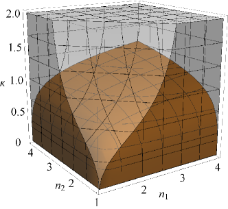
a) b)

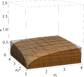
Figure 2: Comparison of the sets of parameters $\kappa,n_{1},n_{2}$ for which the state of two ensembles remains separable (brown inner region), with the ranges of parameters for which it is not detected by the spin variance inequality (5af) with $\lambda=1$ (gray outer region). In figure a) we consider the state produced in the setup in figure 1a, whereas in figures b) the one produced in two steps schematically depicted in figures 1a and 1b.

Interesting enough such measurement induced entanglement between two atomic samples can be deleted by exploiting the squeezing and anti-squeezing effects produced by the laser beams for pure state entanglement[15]. Here we demonstrate that this is also true when the initial states are thermal, however, the procedure has to be slightly modified. Let us consider the state represented by the covariance matrix (5ad). Interaction with a second light beam impinging on each atomic sample at $\alpha_{1}=\alpha_{2}=\pi/2$ (as depicted in Figure 1c) followed by the light measurement will erase the entanglement produced by the interaction with the first light beam if the properties of light are appropriately adjusted. To this aim, it is sufficient to impose a second light beam characterized by the covariance matrix

$$\gamma_{L}=\left(\begin{array}[]{cc}(\triangle x_{1})^{2}&0\\ 0&(\triangle p_{1})^{2}\\ \end{array}\right),$$ (5al)

with

$$(\triangle x_{1})^{2}=\kappa^{2}n_{1}+\kappa^{2}n_{2}+n_{1}n_{2}$$

$$(\triangle p_{1})^{2}=\frac{n_{1}n_{2}}{\kappa^{2}n_{1}+\kappa^{2}n_{2}+1}.$$ (5am)

and interaction coupling $\kappa$. The covariance matrix of the final state is given by:

$$\gamma_{\mathrm{er}}=\left(\begin{array}[]{cccc}\frac{\kappa^{2}n_{2}+n_{1}\left(\kappa^{2}+n_{2}\right)}{2\kappa^{2}+n_{2}}&0&0&0\\ 0&\frac{n_{1}\left(2\kappa^{2}n_{2}+1\right)}{\kappa^{2}\left(n_{1}+n_{2}\right)+1}&0&0\\ 0&0&\frac{\kappa^{2}n_{2}+n_{1}\left(\kappa^{2}+n_{2}\right)}{2\kappa^{2}+n_{1}}&0\\ 0&0&0&\frac{n_{2}\left(2\kappa^{2}n_{1}+1\right)}{\kappa^{2}\left(n_{1}+n_{2}\right)+1}\end{array}\right),$$ (5an)

and the corresponding displacement is:

$$d_{\mathrm{er}}=\left\{-\frac{\tilde{x}_{L,2}\kappa}{2\kappa^{2}+n_{2}},-\frac{\tilde{x}_{L,1}\kappa n_{1}}{\kappa^{2}\left(n_{1}+n_{2}\right)+1},-\frac{\tilde{x}_{L,2}\kappa}{2\kappa^{2}+n_{1}},-\frac{\tilde{x}_{L,1}\kappa n_{1}}{\kappa^{2}\left(n_{1}+n_{2}\right)+1}\right\},$$ (5ao)

where $\tilde{x}_{L,2}$ is the measurement outcome. Note that the state (5an) is separable. It will be identical to the initial one, however, only if $n_{2}=n_{1}$.

3.2 Multipartite bound entanglement

We move now to the truly multipartite entanglement and focus on the simplest case of the 3 atomic samples. We aim at analyzing bound entanglement, which exist only in the mixed state case. The classification of tripartite entanglement in CV was given by Giedke and coworkers in [20], where five classes of states were distinguished. Following their classification, inseparable states with respect to every bipartite splitting are denoted as class 1. States which are biseparable with respect to one (and only one) bipartition belong to class 2. States that are biseparable with respect to two or three bipartitions, but still entangled, belong to class 3 and class 4, respectively. These two classes of states are bound entangled. Finally, class 5 are the separable states.

Continuous-variable cluster-like states can be a universal resource for optical quantum computation[40, 41, 42]. They are defined by analogy with the discrete cluster states generated via Ising interactions between qubits [42]. One can associate the modes of the $N$-mode (CV) system with the vertices of a graph $G$. And the cluster corresponds to a connected graph[43]. For continuous variables, cluster states are defined only asymptotically as those with infinite squeezing in the variables

$$\hat{p}_{a}-\sum_{b\in N_{a}}\hat{x}_{b}$$ (5ap)

for all the modes belonging to the graph, where $N_{a}$ denotes the set of neighbors of vertex $a$. Cluster-like states are defined when the squeezing is finite.

It is possible to create such states with atomic ensembles in the proper geometrical setup [15] taking the samples in the initial vacuum state. The protocol consists of interaction with light passing through the samples at specified angles (see Table 1) plus a homodyne detection of light. Here we check the properties of the states obtained through the same procedure, however for initially thermal samples, i.e., $\gamma_{in}^{(0)}=n\hat{1}_{6}\oplus\hat{1}_{2}$. We demonstrate that in such setup bound entangled states are produced for certain choices of temperature and coupling. The presence of undistillable entanglement in thermal finite-dimensional systems was considered in [44].

We analyze the two cluster states, the linear one and the triangular one, focusing on how the temperature destroys the genuine tripartite entanglement. To discriminate class 1, 2 and 3, the PPT criterion is enough. To discriminate between class 4 and 5 we will use the operational necessary and sufficient criterion for full separability given in [20].

	Linear			Triangular			Smolin state
beam	$\alpha_{1}$	$\alpha_{2}$	$\alpha_{3}$	$\alpha_{1}$	$\alpha_{2}$	$\alpha_{3}$	$\alpha_{1}$	$\alpha_{2}$	$\alpha_{3}$	$\alpha_{4}$
1	0	$\frac{\pi}{2}$	-	$0$	$\frac{\pi}{2}$	$\frac{\pi}{2}$	$0$	$0$	$\pi$	$\pi$
2	$\frac{\pi}{2}$	0	$\frac{\pi}{2}$	$\frac{\pi}{2}$	$0$	$\frac{\pi}{2}$	$\frac{\pi}{2}$	$\frac{\pi}{2}$	$-\frac{\pi}{2}$	$-\frac{\pi}{2}$
3	-	$\frac{\pi}{2}$	$0$	$\frac{\pi}{2}$	$\frac{\pi}{2}$	$0$	-	-	-	-

Table 1: Parameters for tripartite cluster states and the four-partite Smolin state.

The results we obtain are summarize in Figure 3 where we depict as a function of the temperature $T$ through $n(T)=1/\tanh\left(\omega/2T\right)$ and coupling $\kappa$, the different entanglement types created between the atomic samples.

For the linear cluster state (figure 3a), for a fixed value of the parameter $\kappa$, the state is NPT with respect to all the three cuts in the interval $0<T<T_{a}$, meaning that it belongs to class 1. For $T_{a}<T<T_{b}$ the state is PPT with respect to the bipartition $2-(1,3)$ and NPT with respect to others. Hence, in it belongs to bound entangled class 3. For $T>T_{b}$ the state becomes PPT with respect to all the cuts. Using the separability criterion found in [20], we find that within the range $T_{b}<T<T_{c}$ the state is class-4, while for $T>T_{c}$ it becomes fully separable.

(a)(b)

Figure 3: Range of parameters for (a) the linear and (b) the triangular cluster state for which it belongs to different entanglement classes (see explanation it the text).

Figure 3b corresponds to the different entanglement classes for a triangular cluster state. In this case, because of the permutational invariance, class 3 is never recovered. Nevertheless a class-4 region still appears between the genuine tripartite and the fully separable states.

3.3 Multipartite unlockable bound entanglement

Here we propose to use the Gaussian randomness that is inherently present in the system due to uncertainty of the outcome of the light measurement. We will show that it is essential to generate the bound entangled Smolin state.

The Smolin state introduced in [27] using qubits is an interesting example of an undistillable multipartite entangled state that can be unlocked if several parties perform a collective measurement and send the outcome to the remaining parties. The Smolin state if form by an equal-weight mixture of products of the four Bell states $\psi_{i}(i=1,\ldots,4)$

$$\varrho_{\mathrm{Smolin}}=\sum_{i=1}^{4}|\psi_{i}\rangle\!\langle\psi_{i}|_{AB}\otimes|\psi_{i}\rangle\!\langle\psi_{i}|_{CD}.$$ (5aq)

One sees that parties $AB$ and $CD$ share the same Bell state but none of the pairs know which one it is. Such state is clearly separable with respect to partition $AB|CD$. Moreover, since it is permutationally invariant, the above statement also holds for every two pairs, not only for $AB$ and $CD$. Hence, according to the definition, the state is undistillable with respect to arbitrary two parties, since there always exists a separable bipartition dividing them.

The fact that arbitrary two pairs share the same unknown Bell state makes the entanglement present in the Smolin state unlockable. Imagine the situation in which two of the parties, say $C$ and $D$, meet in one laboratory and perform collectively a measurement in the Bell basis, identifying thus the state they possess. This measurement projects the state shared by $AB$ on the one corresponding to the outcome of the parties $CD$. Hence, if $A$ and $B$, still being in separate laboratories, obtain (by classical communication) the information about the outcome of $CD$, they can use their maximally entangled state. We emphasize that the otherwise unknown Bell state is useless.

The Smolin state possesses many other interesting features. Apart from being unlockable, its entanglement can be activated [45] through a cooperation of five parties sharing two copies of the state. Despite being bound entangled, this state can be used in the remote quantum information concentration protocol [46] and maximally violates a Bell inequality being at the same time useless for the secret key distillation [23].

Recently, Zhang has generalized the discrete Smolin state to the Gaussian CV scenario using the mathematical formalism of stabilizers [28]. It turns out that the state proposed by Zhang can indeed be understood as some mixture of products of the continuous variables EPR-like states in this way. Let us consider two EPR(-like) states with known reference displacement and randomly displace both of them in the opposite unknown directions in the phase space, as schematically depicted in figure 4. The only constraint imposed on the random displacement is that it has a Gaussian distribution. In this way we obtain a Gaussian mixture of two displaced EPR pairs.

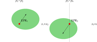
Figure 4: Schematically depicted Smolin state in the phase space. The red dots correspond to the EPR-like states, the green ellipses represent the random Gaussian displacement that depends on the properties of light passing through the samples.

The properties of the CV Smolin state are slightly different from those of the qubit state. Firstly and most importantly, we loose the permutational invariance [28]. Secondly, since the maximally entangled EPR-state corresponds to infinite squeezing in the CV and is not physical, we will always have to deal with ”EPR-like” states and therefore it is necessary to analyze the effect of the finite squeezing on the properties of the final Smolin-like state. Both of the above constraints force the Smolin-like state to be undistillable only with respect to chosen parties and within a particular range of the squeezing parameter.

Let us demonstrate how the mathematical setup generating the Smolin-like state proposed in [28] greatly simplifies in the atomic-ensemble realization. We characterize each step of the procedure using the covariance matrix and the displacement vector. Finally, using the symplectic formalism, we demonstrate the unlocking protocol.

From now on we will distinguish the parties (modes) with Latin numbers. As demonstrated by Zhang, the Smolin-like state can be generated in two steps:

(i) generate two EPR-like pairs with reduced fluctuations (squeezing) in $\hat{x}_{1}+\hat{x}_{2}$ and $\hat{p}_{1}-\hat{p}_{2}$ ($\hat{x}_{3}+\hat{x}_{4}$ and $\hat{p}_{3}-\hat{p}_{4}$ for modes $3$ and $4$) and known displacement

(ii) displace the EPR pairs by random Gaussian variables $\lambda_{1}$ and $\lambda_{2}$ such that the quadratures transform in the following way:

$$\hat{x}_{1}+\hat{x}_{2}+\hat{x}_{3}+\hat{x}_{4}\rightarrow(\hat{x}_{1}-\lambda_{1})+(\hat{x}_{2}-\lambda_{1})+(\hat{x}_{3}+\lambda_{1})+(\hat{x}_{4}+\lambda_{1}),$$ (5ar)

and

$$\hat{p}_{1}-\hat{p}_{2}+\hat{p}_{3}-\hat{p}_{4}\rightarrow(\hat{p}_{1}+\lambda_{2})-(\hat{p}_{2}-\lambda_{2})+(\hat{p}_{3}-\lambda_{2})-(\hat{p}_{4}+\lambda_{2}).$$ (5as)

Note that indeed the squeezed combinations in modes $1-2$ and $3-4$ are displaced in the opposite directions. Implementation of each of these steps is experimentally feasible in the geometrical setup of atomic ensembles. Step (i) concerns the generation of EPR-like states with known displacement which is easily achieved (see also [15]). Step (ii) concerns the generation of a random Gaussian variables in the displacements. In our geometrical setup this can be achieved by shining two light beams at some given angles as summarized in table 1. A straightforward application shows that the angles reported in the above table modify the the quadratures of atomic spin ensembles in the following way:

$$\hat{x}_{1}+\hat{x}_{2}+\hat{x}_{3}+\hat{x}_{4}\rightarrow(\hat{x}_{1}-\kappa\hat{p}_{L,1})+(\hat{x}_{2}-\kappa\hat{p}_{L,1})+(\hat{x}_{3}+\kappa\hat{p}_{L,1})+(\hat{x}_{4}+\kappa\hat{p}_{L,1})$$ (5at)

and

$$\hat{p}_{1}-\hat{p}_{2}+\hat{p}_{3}-\hat{p}_{4}\rightarrow(\hat{p}_{1}+\kappa\hat{p}_{L,2})-(\hat{p}_{2}-\kappa\hat{p}_{L,2})+(\hat{p}_{3}-\kappa\hat{p}_{L,2})-(\hat{p}_{4}+\kappa\hat{p}_{L,2}).$$ (5au)

Comparing now equations (5ar) and (5as) to equations (5at) and (5au) respectively, one observes that our setup reproduces precisely the required displacements. Now, if the output light is not measured, $\kappa\hat{p}_{L,1}$ and $\kappa\hat{p}_{L,2}$ remain unknown random Gaussian variables with expectation value and variance that can be easily adjusted by choosing the input light with specific properties (vacuum squeezed, thermal etc.). From now on we will denote this random variables by $\bar{p}_{L,1},\bar{p}_{L,2}$.

We switch to the covariance matrix formalism that allows us to get a better insight into the process and the properties of the final state. We begin directly with two $EPR$ pairs with zero reference displacement and characterized by the squeezing parameter $r$, and a general light mode characterized by the variances: $\left(\Delta\hat{x}_{L,1}\right)^{2},\left(\Delta\hat{p}_{L,1}\right)^{2}$ and zero displacement. The initial state of the setup is described by:

$$\gamma_{1}^{(\mathrm{in})}=\gamma_{\mathrm{EPR_{1}}}\oplus\gamma_{\mathrm{EPR_{2}}}\oplus\left(\begin{array}[]{cc}\left(\Delta\hat{x}_{L,1}\right)^{2}&0\\ 0&\left(\Delta\hat{p}_{L,1}\right)^{2}\\ \end{array}\right).$$ (5av)

The interaction between the atomic ensembles and the light leads to the following CM for atoms

$$\gamma_{1}^{(\mathrm{out})}=\left(\begin{array}[]{cccccccc}a_{1}&0&c_{1}&0&e_{1}&0&e_{1}&0\\ 0&b&0&d&0&0&0&0\\ c_{1}&0&a_{1}&0&e_{1}&0&e_{1}&0\\ 0&d&0&b&0&0&0&0\\ e_{1}&0&e_{1}&0&a_{1}&0&c_{1}&0\\ 0&0&0&0&0&b&0&d\\ e_{1}&0&e_{1}&0&c_{1}&0&a_{1}&0\\ 0&0&0&0&0&d&0&b\end{array}\right)$$ (5be)

$$\mathrm{with}$$

$$a_{1}=\kappa^{2}\left(\Delta\hat{p}_{L,1}\right)^{2}+\mathrm{ch}2r,\quad b=\mathrm{ch}2r\quad c_{1}=\kappa^{2}\left(\Delta\hat{p}_{L,1}\right)^{2}-\mathrm{sh}2r,$$

$$d=\kappa^{2}\left(\Delta\hat{p}_{L,1}\right)^{2}-\mathrm{ch}2r\quad e_{1}=-\kappa^{2}\left(\Delta\hat{p}_{L,1}\right)^{2}.$$

Interaction with a second mode of light characterized by variances $\left(\Delta\hat{x}_{L,2}\right)^{2},\left(\Delta\hat{p}_{L,2}\right)^{2}$, leads to the CM:

$$\gamma_{2}^{(\mathrm{out})}=\left(\begin{array}[]{cccccccc}a_{1}&0&c_{1}&0&e_{1}&0&e_{1}&0\\ 0&a_{2}&0&-c_{2}&0&e_{2}&0&-e_{2}\\ c_{1}&0&a_{1}&0&e_{1}&0&e_{1}&0\\ 0&-c_{2}&0&a_{2}&0&-e_{2}&0&e_{2}\\ e_{1}&0&e_{1}&0&a_{1}&0&c_{1}&0\\ 0&e_{2}&0&-e_{2}&0&a_{2}&0&-c_{2}\\ e_{1}&0&e_{1}&0&c_{1}&0&a_{1}&0\\ 0&-e_{2}&0&e_{2}&0&-c_{2}&0&a_{2}\end{array}\right)$$ (5bn)

$$a_{1}=\kappa^{2}\left(\Delta\hat{p}_{L,1}\right)^{2}+\mathrm{ch}2r,\quad a_{2}=\kappa^{2}\left(\Delta\hat{p}_{L,2}\right)^{2}+\mathrm{ch}2r,$$

$$c_{1}=\kappa^{2}\left(\Delta\hat{p}_{L,1}\right)^{2}-\mathrm{sh}2r,\quad c_{2}=\kappa^{2}\left(\Delta\hat{p}_{L,2}\right)^{2}-\mathrm{sh}2r,$$

$$e_{1}=-\kappa^{2}\left(\Delta\hat{p}_{L,1}\right)^{2},\quad e_{2}=-\kappa^{2}\left(\Delta\hat{p}_{L,2}\right)^{2}.$$

and the displacement of the final state is given by:

$$d_{2}^{(\mathrm{out})}=\left(-\kappa\bar{p}_{L,1},\kappa\bar{p}_{L,2},-\kappa\bar{p}_{L,1},-\kappa\bar{p}_{L,2},\kappa\bar{p}_{L,1},-\kappa\bar{p}_{L,2},\kappa\bar{p}_{L,1},\kappa\bar{p}_{L,2}\right).$$ (5bo)

We verify separability of the obtained state using the partial time reversal criterion and see that the state:
(i) it is always $PPT$ with respect to partition $12|34$,
(ii) it is always $NPT$ with respect to partition $13|24$,
(iii) it is $PPT$ with respect to partition $14|23$ only if

$$\kappa^{2}\left(\Delta\hat{p}_{L,1}\right)^{2}\geq\frac{1}{4}\left(e^{2r}-e^{-2r}\right)\;\mathrm{or}\;\kappa^{2}\left(\Delta\hat{p}_{L,2}\right)^{2}\geq\frac{1}{4}\left(e^{2r}-e^{-2r}\right);$$ (5bp)

(iv) all the partitions one vs. three modes are always $NPT$, in agreement with the results obtained in [28].
An important thing to notice is that the state is unlockable bound entangled only if the partition $14|23$ is $PPT$, since only in this case the entanglement between modes $1$ and $2$ is bound and the unlocking procedure makes sense.

In order to show the unlockability of the obtained state, we write the CM and displacement in the basis in which the EPR states are diagonal, i.e., $(1/\sqrt{2})\left(\hat{x}_{1}+\hat{x}_{2},\ldots,\hat{p}_{3}-\hat{p}_{4}\right)$. For simplicity we also assume that $\left(\Delta\hat{x}_{L,1}\right)^{2}=\left(\Delta\hat{x}_{L,2}\right)^{2}=\left(\Delta\hat{x}_{L}\right)^{2}$ and $\left(\Delta\hat{p}_{L,1}\right)^{2}=\left(\Delta\hat{p}_{L,2}\right)^{2}=\left(\Delta\hat{p}_{L}\right)^{2}$ then

$$\gamma_{\mathrm{S}}=\left(\begin{array}[]{cccccccc}e^{-2r}+f&0&0&0&-f&0&0&0\\ 0&e^{2r}&0&0&0&0&0&0\\ 0&0&e^{2r}&0&0&0&0&0\\ 0&0&0&e^{-2r}+f&0&0&0&-f\\ -f&0&0&0&e^{-2r}+f&0&0&0\\ 0&0&0&0&0&e^{2r}&0&0\\ 0&0&0&0&0&0&e^{2r}&0\\ 0&0&0&-f&0&0&0&e^{-2r}+f\end{array}\right)$$ (5by)

$$f=2\kappa^{2}\left(\Delta\hat{p}_{L}\right)^{2}$$

$$d_{\mathrm{S}}=\left\{-\sqrt{2}\kappa\bar{p}_{L,1},0,0,\sqrt{2}\kappa\bar{p}_{L,2},\sqrt{2}\kappa\bar{p}_{L,1},0,0,-\sqrt{2}\kappa\bar{p}_{L,2}\right\}$$ (5bz)

Now inspection of $\gamma_{s}$ shows clearly that we have two correlated $EPR$ pairs displaced by random vectors pointing in the opposite directions in the phase space of the squeezed variables, exactly as depicted in figure 4. Since we do not know where in the phase space are the EPR pairs, we cannot use them for quantum tasks. Therefore, by analogy to the discrete case [27, 23], unlocking of entanglement is understood as learning which of the displaced $EPR$ pairs is shared by pair $1-2$ by measuring the displacement of the other EPR pair shared by $3-4$.

For completeness we also demonstrate all the steps of the unlocking protocol with the atom-light interface using the symplectic formalism. The measurement of $\hat{x}_{3}+\hat{x}_{4}$ and $\hat{p}_{3}-\hat{p}_{4}$ can be done with two probe light beams with reduced fluctuations in $x_{P}$, i.e., $\left(\Delta x_{P}\right)^{2}<\hbar/2$ (QND measurement) [47]. The probe beams pass through the samples $3-4$ at the angles $\alpha_{3}^{(1)}=\alpha_{4}^{(1)}=\pi/2$ and $\alpha_{3}^{(2)}=0,\alpha_{4}^{(2)}=\pi$, respectively, and are measured afterwards. If the measurement outcomes are, respectively, $x_{+}$, $p_{-}$, the final state of modes $1-2$ is characterized by the following CM and displacement (still in the $EPR$ basis):

$$\gamma_{12}=\left(\begin{array}[]{cccc}\frac{f\left(2\kappa^{2}+e^{2r}\left(\Delta\hat{x}_{P}\right)^{2}\right)}{e^{2r}\left(2\kappa^{2}f+\left(\Delta\hat{x}_{P}\right)^{2}\right)+2\kappa^{2}}+e^{-2r}&0&0&0\\ 0&e^{2r}&0&0\\ 0&0&e^{2r}&0\\ 0&0&0&\frac{f\left(2\kappa^{2}+e^{2r}\left(\Delta\hat{x}_{P}\right)^{2}\right)}{e^{2r}\left(2\kappa^{2}f+\left(\Delta\hat{x}_{P}\right)^{2}\right)+2\kappa^{2}}+e^{-2r}\end{array}\right),$$ (5ca)

$$d_{12}=\sqrt{2}\kappa\times\left[x_{+}g-\bar{p}_{L,1},0,0,p_{-}g+\bar{p}_{L,2}\right],$$ (5cb)

$$g=\frac{f}{\left(\Delta\hat{x}_{P}\right)^{2}+2\kappa^{2}(e^{-2r}+f)}$$

If the variables $\hat{x}_{3}+\hat{x}_{4}$ and $\hat{p}_{3}-\hat{p}_{4}$ are strongly enough squeezed, the obtained outcome approximates well the displacement of $\hat{x}_{1}+\hat{x}_{2}$ and $\hat{p}_{1}-\hat{p}_{2}$. Therefore, we may write $2\kappa\bar{p}_{L,1}=-x_{+}$ and $2\kappa\bar{p}_{L,2}=-p_{-}$. In this way the resulting displacement is a function of the known parameters

$$\tilde{d}_{12}=\sqrt{2}\left[x_{+}\left(\kappa g+\frac{1}{2}\right),0,0,p_{-}\left(\kappa g-\frac{1}{2}\right)\right].$$ (5cc)

In comparison to the initial EPR state, the covariance matrix (5ca) has an additional positive term in diagonal elements, which reads

$$\delta=\frac{f\left(2\kappa^{2}+e^{2r}\left(\Delta\hat{x}_{P}\right)^{2}\right)}{e^{2r}\left(2\kappa^{2}f+\left(\Delta\hat{x}_{P}\right)^{2}\right)+2\kappa^{2}}.$$ (5cd)

It increases the variance of the squeezed variables and therefore makes the state mixed and less entangled. In order to quantify the entanglement in the final unlocked state, we assume that the coupling constants $\kappa$ used in the preparation of the EPR states and the ones used for generation and unlocking of the Smolin state are equal and we express them in terms of the squeezing parameter $r$

$$\kappa^{2}=(1+\rme^{2r})/2.$$ (5ce)

Further we assume that the squeezing of the probe light beam is the same as the squeezing of initial EPR pairs, i.e., $\left(\Delta\hat{x}_{P}\right)^{2}=e^{-2r}$. In this way, the properties of the final state depend only on two parameters: $r$ and $\left(\Delta\hat{p}_{L}\right)^{2}$. In figure 5 we plot the negativity of the unlocked state, as a function of these parameters. For the admissible values of $r$, the negativity of the final state is roughly a half of the value for the initial EPR pair.

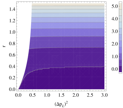
Figure 5: Negativity of the unlocked state given by equation (5cb) as a function of the squeezing parameter $r$ and variance of the random displacement $\left(\Delta\hat{p}_{L}\right)^{2}$. All the other parameters are expressed in terms of $r$ (see explanation in the text).

4 Conclusions

Our results can be summarize us follows. We have shown that, unlike in the pure state case, if the atomic ensembles are initially in a thermal state the entangling procedure only succeeds for certain choices of the coupling parameter. In this way we have provided bounds on the experimental parameters leading to mixed state entanglement. Further we have shown that tripartite continuous cluster-like states are robust against initial thermal noise present in the atomic ensembles, meaning that there exists a finite range of temperatures for which the final state remains genuine tripartite entangled. We have also demonstrate that with increasing temperature, the states becomes bound entangled and finally fully separable.

Finally, we have also shown that a mixed state of atomic ensembles can be produced from an initial pure state if the light beam is not measured after the interaction. In this case, the interaction with the light beam mixes all the possible outcomes with a Gaussian weight. Using this procedure, starting from two pure bipartite entangled states, it is possible to produce the so-called Smolin state which is an example of an unlockable bound entangled state. It should be emphasized that, since this procedure does not involve the final projective measurement, it cannot produce extra entanglement. Its only effect is introducing randomness in the system, making the entanglement bound.

Summarizing, our analysis shows that atomic ensembles offer a versatile toolbox for generation and manipulation of multipartite entanglement both in the pure and mixed state cases. By exploiting further the geometrical setting introduced in [15] we have been able to assess the robustness of the entangling schemes to set guidelines for future experiments, both in the bipartite as well as in the multipartite case. Moreover, we have demonstrated that the very same setting provides experimentally feasible schemes for generation of bound entanglement, broadening the applicability of atomic ensembles for quantum information studies. In particular, our results provide, to the best of our knowledge, the first experimentally feasible realization of the Smolin state with continuous variables (for qubit realization see [48]).

References

References

- [1] A Kuzmich, K Mølmer, and ES Polzik. Spin squeezing in an ensemble of atoms illuminated with squeezed light. Phys. Rev. Lett., 79:4782, 1997.
- [2] A. Kuzmich, L. Mandel, and N. P. Bigelow. Generation of spin squeezing via continuous quantum nondemolition measurement. Phys. Rev. Lett., 85:1594, 2000.
- [3] B Julsgaard, J Sherson, J I Cirac, J Fiurášek, and E S Polzik. Experimental demonstration of quantum memory for light. Nature, 432:482, 2004.
- [4] B Julsgaard, A Kozhekin, and ES Polzik. Experimental long-lived entanglement of two macroscopic objects. Nature (London), 413:400, 2001.
- [5] M Napolitano and M W Mitchell. Nonlinear metrology with a quantum interface. New Journal of Physics, 12:093016, 2010.
- [6] M Napolitano, M Koschorreck, B Dubost, N Behbood, R J Sewell, and M W Mitchell. Interaction-based quantum metrology showing scaling beyond the Heisenberg limit. Nature, 471:486, 2011.
- [7] F Wolfgramm, A Cerè, F A Beduini, A Predojević, M Koschorreck, and M W Mitchell. Squeezed-light optical magnetometry. Phys. Rev. Lett., 105:053601, 2010.
- [8] K Eckert, Ł Zawitkowski, A Sanpera, M Lewenstein, and E Polzik. Quantum Polarization Spectroscopy of Ultracold Spinor Gases. Physical Review Letters, 98:100404, 2007.
- [9] K Eckert, O Romero-Isart, M Rodriguez, M Lewenstein, ES Polzik, and A Sanpera. Quantum non-demolition detection of strongly correlated systems. Nature Physics, 4:50, 2007.
- [10] T Roscilde, M Rodríguez, K Eckert, O Romero-Isart, M Lewenstein, E Polzik, and A Sanpera. Quantum polarization spectroscopy of correlations in attractive fermionic gases. New Journal of Physics, 11:055041, 2009.
- [11] G de Chiara, O Romero-Isart, and A Sanpera. in preparation.
- [12] D Greif, L Tarruell, T Uehlinger, R Jördens, and T Esslinger. Probing nearest-neighbor correlations of ultracold fermions in an optical lattice. Phys. Rev. Lett., 106:145302, 2011.
- [13] L-H Duan, G Giedke, JI Cirac, and P Zoller. Inseparability criterion for continuous variable systems. Phys. Rev. Lett., 84:2722, 2000.
- [14] P van Loock and A Furusawa. Detecting genuine multipartite continuous-variable entanglement. Phys. Rev. A, 67:052315, 2003.
- [15] J Stasińska, C Rodó, S Paganelli, G Birkl, and A Sanpera. Manipulating mesoscopic multipartite entanglement with atom-light interfaces. Phys. Rev. A, 80:062304, 2009.
- [16] D Bruß and C Macchiavello. Multipartite entanglement in quantum algorithms. Phys. Rev. A, 83:052313, 2011.
- [17] L Memarzadeh, Ch Macchiavello, and S Mancini. Recovering quantum information through partial access to the environment. New Journal of Physics, 13:103031, 2011.
- [18] M Bremner, C Mora, and A Winter. Are Random Pure States Useful for Quantum Computation? Physical Review Letters, 102:11, 2009.
- [19] W Dür, J I Cirac, and R Tarrach. Separability and Distillability of Multiparticle Quantum Systems. Phys. Rev. Lett., 83:3562, 1999.
- [20] G Giedke, B Kraus, M Lewenstein, and JI Cirac. Separability properties of three-mode gaussian states. Phys. Rev. A, 64:052303, 2001.
- [21] K G H. Vollbrecht and M M Wolf. Activating distillation with an infinitesimal amount of bound entanglement. Phys. Rev. Lett., 88:247901, 2002.
- [22] K Horodecki, M Horodecki, P Horodecki, and J Oppenheim. Secure key from bound entanglement. Phys. Rev. Lett., 94:160502, 2005.
- [23] R Augusiak and P Horodecki. Bound entanglement maximally violating bell inequalities: Quantum entanglement is not fully equivalent to cryptographic security. Phys. Rev. A, 74:010305, 2006.
- [24] Ll Masanes. All bipartite entangled states are useful for information processing. Phys. Rev. Lett., 96:150501, 2006.
- [25] Ll Masanes, Yeong-Cherng Liang, and Andrew C. Doherty. All bipartite entangled states display some hidden nonlocality. Phys. Rev. Lett., 100:090403, 2008.
- [26] M Piani and J Watrous. All entangled states are useful for channel discrimination. Phys. Rev. Lett., 102:250501, 2009.
- [27] J A Smolin. Four-party unlockable bound entangled state. Phys. Rev. A, 63:032306, 2001.
- [28] Jing Zhang. Continuous-variable multipartite unlockable bound entangled gaussian states. Phys. Rev. A, 83:052327, 2011.
- [29] J Sherson and K Mølmer. Entanglement of large atomic samples: A gaussian-state analysis. Phys. Rev. A, 71:033813, 2005.
- [30] LB Madsen and K Mølmer. Spin squeezing and precision probing with light and samples of atoms in the gaussian description. Phys. Rev. A, 70:052324, 2004.
- [31] K Hammerer, A S Sørensen, and E S Polzik. Quantum interface between light and atomic ensembles. Reviews of Modern Physics, 82:1041, 2010.
- [32] M Koschorreck and M W Mitchell. Unified description of inhomogeneities, dissipation and transport in quantum light-atom interfaces. Journal of Physics B: Atomic, Molecular and Optical Physics, 42:195502, 2009.
- [33] G Giedke and JI Cirac. Characterization of gaussian operations and distillation of gaussian states. Phys. Rev. A, 66:032316, 2002.
- [34] SL Braunstein and P van Loock. Quantum information with continuous variables. Rev. Mod. Phys., 77:513, 2005.
- [35] G Adesso and F Illuminati. Entanglement in continuous-variable systems: recent advances and current perspectives. J. Phys. A: Math. Theor., 40:7821, 2007.
- [36] J Eisert, S Scheel, and MB Plenio. Distilling gaussian states with gaussian operations is impossible. Phys. Rev. Lett., 89:137903, 2002.
- [37] M Horodecki, P Horodecki, and R Horodecki. Separability of mixed states: necessary and sufficient conditions. Physics Letters A, 223:1, 1996.
- [38] A Peres. Separability criterion for density matrices. Phys. Rev. Lett., 77:1413, 1996.
- [39] R Simon. Peres-horodecki separability criterion for continuous variable systems. Phys. Rev. Lett., 84:2726, 2000.
- [40] MA Nielsen. Optical quantum computation using cluster states. Phys. Rev. Lett., 93:040503, 2004.
- [41] M Ohliger, K Kieling, and J Eisert. Limitations of quantum computing with gaussian cluster states. Phys. Rev. A, 82:042336, 2010.
- [42] L Aolita, A Roncaglia, A Ferraro, and A Acín. Gapped Two-Body Hamiltonian for Continuous-Variable Quantum Computation. Physical Review Letters, 106, 2011.
- [43] HJ Briegel and R Raussendorf. Persistent entanglement in arrays of interacting particles. Phys. Rev. Lett., 86:910, 2001.
- [44] D Cavalcanti, L Aolita, a Ferraro, a García-Saez, and a Acín. Macroscopic bound entanglement in thermal graph states. New Journal of Physics, 12:025011, 2010.
- [45] P W Shor, J A Smolin, and A V Thapliyal. Superactivation of bound entanglement. Phys. Rev. Lett., 90:107901, 2003.
- [46] M Murao and V Vedral. Phys. Rev. Lett., 86:352, 2001.
- [47] JL Sørensen, J Hald, and ES Polzik. Quantum noise of an atomic spin polarization measurement. Phys. Rev. Lett., 80:3487, 1998.
- [48] E Amselem and M Bourennane. Experimental four-qubit bound entanglement. Nature Physics, 5:748, 2009.